
In silico characterization of the effects of size, distribution, and modulus contrast of aortic focal softening on pulse wave propagations
- DOI
- 10.1016/j.artres.2015.04.002How to use a DOI?
- Keywords
- Aortic pulse wave; Aortic wall inhomogeneity; Disease biomarker; Minimally-invasive diagnosis
- Abstract
Examining the change in regional stiffness of the arterial wall may prove as a reliable method for detecting various cardiovascular diseases. As suggested by Moens–Korteweg relationship, the pulse wave velocity (PWV) along the arteries has been shown to correlate to the stiffness of the arterial wall; the higher the stiffness, the higher the PWV. The current primary clinical practice of obtaining an average PWV between remote sites such as femoral and carotid arteries is not as clinically effective, since various cardiovascular diseases are shown to be accompanied by focal changes in stiffness. Therefore, methods to examine the PWVs focally are warranted. Extending on the findings of previous studies, pulse wave propagations along aortas with wall focal softening were addressed in this study using two-way coupled fluid–structure interaction (FSI) simulations of arterial pulsatile motions. Spatio-temporal maps of the wall displacement were used to evaluate the regional pulse wave propagations and velocities. In particular, soft wall inclusions of different number, size, and modulus were examined. The findings showed that the qualitative markers on the pattern of the wave propagations such as the existence of forward, reflected, and standing waves, as well as the quantitative markers such as PWV, linear coefficient of the propagating waves, and the width of the standing waves, provide a reliable tool to distinguish between the natures of the wall focal softening. Future studies are needed to include physiologically-relevant wall inhomogeneity in order to further implicate on the clinical potentials of the inverse problem for noninvasive diagnosis.
- Copyright
- © 2015 Association for Research into Arterial Structure and Physiology. Published by Elsevier B.V. All rights reserved.
- Open Access
- This is an open access article distributed under the CC BY-NC license.
Introduction
The majority of cardiovascular diseases (CVDs) have been shown to be accompanied by alterations in mechanical properties of the arterial wall.1 Changes in aortic wall stiffness has been widely agreed as an independent indicator of CVDs such as aortic calcification and aneurysm.2–10 Determining arterial stiffness has been known to be a part of clinical diagnosis, therapy, and follow up procedures.11,12 The established concept based on the Moens–Korteweg relationship has proven that the velocity of the aortic pulse wave is correlated to the arterial stiffness; the stiffer the wall, the higher the pulse wave velocity (PWV),13–15 and therefore can be used to estimate the wall stiffness noninvasively based on PWV measurements. Current clinical practice for measuring the PWV includes acquiring the temporal pulse pressure profiles at carotid and femoral artery sites11,16 and then obtaining the average PWV via dividing the over-the-skin distance by the time delay between the two pulse profiles.17,18 There are various inaccuracies associated with this method mostly due to the incorrect arterial geometry and/or assuming a single longitude flow direction between the carotid and femoral arteries which leads to an underestimation or overestimation of the true traveled distance and the PWV therein.11,19 Furthermore, the wall stiffness has been shown to vary locally along the artery20 which makes an average PWV not properly representing or detecting the associated stiffness variations. Therefore, this current clinical practice may prove not efficient in diagnosing a majority of CVDs initiation and progression that have been shown to entail focal tissue degradation.21–23
Several approaches have been taken to overcome the aforementioned issues. The first approach is to use mathematical models for providing a local approximation of the PWV using measurable parameters such as blood pressure, velocity, arterial diameter, flow rate, and luminal area.24 The second approach includes an ultrasound based method of Pulse Wave Imaging (PWI), which also provides a local estimate of the PWV,25,26 with the feasibility studies shown on different frontiers such as animal studies in vivo and in vitro, phantom studies, and clinical studies.27–32 The efficacy and reliability of both methods to pathological conditions involving high focal variations has been found compromised since such wall variations create complex wave propagation dynamics consisting of multiple forward and reflected waves that make the wave quantification and PWV measurement challenging.27,32–34 In order to shed light on the pulsatile wave dynamics in aortas with focal inhomogeneities, Fluid Structure Interaction (FSI) simulations could be very helpful. The feasibility of using Coupled Eulerian Lagrangian (CEL) solver of Abaqus (Simulia, RI, USA) in modeling fluid-induced aortic pulse waves has been shown with findings being validated against phantom and in vitro studies.30,31 Particularly, recent studies have shown the efficacy of CEL-based simulations in reliably detecting the existence of focal stiffening and softening of the aortic walls.35 In addition, a further study confirms the establishment of qualitative and quantitative markers that are present when stiffening heterogeneities of the wall is created in terms of number, size, and modulus of focal hard inclusions,36 which can potentially be used for PWI-based diagnosis purposes. Building on the infrastructure of the previous studies, this study further extends the quantified findings on the pulse wave propagations to the aortas with wall focal softening, aiming at identifying the relevant diagnostic markers.
Methods
Computational modeling
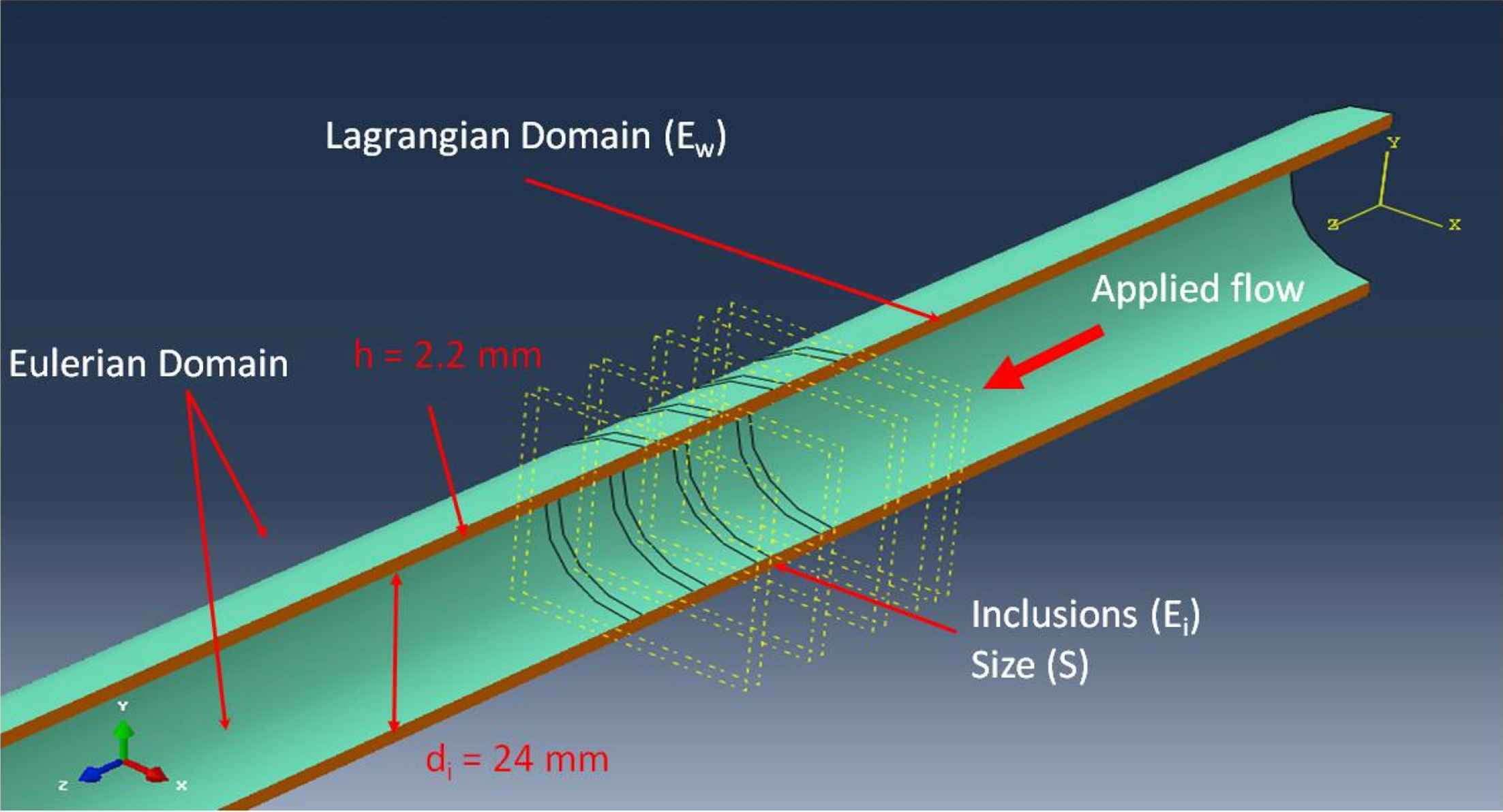
A Dell Precision™ with Intel Core i7-3840QM and 32 GB Ram was used to perform dynamic two-way Fluid Structure Interaction (FSI) simulations of pulse wave propagations along the walls of a 3D aortic geometry. The Coupled Eulerian-Lagrangian (CEL) explicit solver of Abaqus 6.11–1 (Simulia, RI, USA) was used to describe the fluid dynamics and to capture the fluid–solid interactions. Defining the initial position of a moving particle in the material at the reference time, the new position of the same particle at the current time and the resulted velocity and acceleration can be obtained either in Lagrangian coordinate system (e.g. such as for the motion of the wall material), or the Eulerian coordinate system (e.g. such as for the motion of the fluid material), and based on the principle of coordinate-invariance, the displacement, velocity and acceleration fields obtained from either coordinate system are equal. In the CEL solver for the finite element method, the motions of the particles in fluid (i.e. flow) are formulated in Eulerian coordinate system, in which the mesh topology consists of elements that are affixed in the space while material is allowed to cross in/out of the element boundaries. However, the motions for the solid (i.e. aortic wall) domains are formulated using Lagrangian coordinate system, where the elements are affixed to and move with the particles during the material deformation. In the present model, the Lagrangian part was constructed as a straight cylindrical geometry (L = 250 mm; di = 24 mm; h = 2.2 mm), with a Young’s modulus of Ew = 5.12 MPa, density of ρw = 1050 kg/m3, and Poisson’s ratio of νw = 0.48.37–39 The Eulerian domain was established to encompass the entire Lagrangian domain in order to accommodate the potential presence of fluid and the FSI thereof on the deformed geometries at all times during the simulation. Without the loss of generality in generating relevant wave dynamics, fluid was assumed to be Newtonian, with material properties as density ρf = 1000 kg/m3, reference sound speed cf = 1483 m/s and viscosity ηf = 0.0001 N/m2.40,41 Boundary conditions on the inlet and outlet were applied as full constraint in all 6 degrees of freedom. A pulse profile with magnitude V0 = 5 m/s was applied as the inlet flow, acting as the drive in generating the FSI-induced pulsatile motions in the wall. The pulse profile is a smooth step function over time. The flow parameters were chosen in consistency with similar numerical and experimental studies,30,31,35,36 primarily in order to induce strong enough displacement in the aortic walls, so the resulted wave propagations would be fully detectable. Step increases in amplitude from 0 to 1 every 0.001 s. A frictionless FSI interface was defined between the wall and the medium. In order to enhance the FSI mesh accuracy, both the Eulerian and Lagrangian domains were meshed using same-size linear hexagonal 3D elements. A seeding size of 2 mm was found to be optimal in both providing a minimum of two layers of elements across the wall thickness at its thinnest sites and in maintaining the low computational cost. The model contained a 23040/34695 elements/nodes for the Lagrangian domain, and 95750/102408 elements/nodes for the Eulerian domain. The time increment was in the order of 6e-05s, and a total simulation time of 15 ms was considered.
Effects of number of inclusions, and inclusion size and modulus contrast
In order to examine the effects of wave inhomogeneities, a homogenous model-as the control-as well as 9 inhomogeneous models with different inhomogeneity parameters were studied. The control model consisted of homogenous wall mechanical properties, namely a Young’s modulus of Ew = 5.12 MPa. As far as the 9 inhomogeneous models were concerned, different set of soft inclusions with varying properties were included in the walls of modulus Ew = 5.12 MPa (Fig. 1). The number of inclusions was denoted by N and examined within the range of N = 1, 2, 3 and 4; each 10 mm apart. The size of the inclusion(s) was shown as S and examined in a range of S = 2, 5, and 10 mm. The modulus of the inclusion(s), Ei, was examined in a range of Ei = 4.10, 3.413, 2.93, and 2.56 MPa, translating into a characteristic parameter of inclusion-to-wall modulus contrast, MC = Ei/Ew, which falls within a corresponding range of MC = 1.25−1, 1.5−1, 1.75−1, and 2−1, respectively. The inclusions were at least 90 mm distant from the flow inlet, allowing for the propagating forward wave to be developed. Figure 2 shows a long-axis cross section of a homogenous model displaying wall displacement during simulation. After completion of the simulations, the radial displacement of the entire wall along the vessel long-axis (axial spatial resolution of 300 mm) was measured on multiple time-points (temporal resolution of 15 ms), capturing the wave peak as the point with maximum displacement. The spatial and temporal information was used to create the spatio-temporal maps, allowing for the visualization and analysis of the entire wave propagation. The Pulse Wave Velocity (PWV) was calculated as the slope of the linear regression fit to any arbitrary characteristic point on the wave. It was found that a point corresponding to 80% of the wave peak (will be arbitrary referred to as the wave foot throughout the rest of the manuscript for simplicity) results in the most smooth and homogenous wave propagation. The spatio-temporal maps were used to analyze the pulse wave propagation both qualitatively (e.g. reflection patterns) and quantitatively (e.g. PWVs and linear correlation coefficients (r2s) on the forward waves).
Long-axis cross-section view of the 3D aortic model showing an example of inhomogeneous walls with N = 4 number of inclusions of size S = 2 mm.

Long-axis cross section view of the (A) 3D aortic geometry and the coupled Eulerian-Lagrangian (CEL) meshing and zoomed in portion of (A) displaying the (B) wave peak. The wall displacement is used to track the pulse; red being the maximum displacement corresponding to the wave peak. (For interpretation of the references to colour in this figure legend, the reader is referred to the web version of this article.)
Results
Homogeneous and inhomogeneous pulse wave propagations
In order to showcase the wave propagation patterns, Fig. 3 depicts the 3D waterfall plots of the displacement in the upper wall motion obtained on homogeneous walls (Fig. 3A) as well as on three instances of inhomogeneous walls with representative sets of inclusion number, size, and modulus contrast (Fig. 3B–D). The plots show the progression of a forward wave that gets disturbed at the site of the soft inclusions and splits into forward and reflected waves. Also, a stationary wave is observed as a result of large displacements of the wall at the constant sites of the inclusions. Reflected and stationary waves are by-products of the inclusions. Detection of reflected and stationary waves confirms that the forward wave is disturbed at the site of the inclusion. Furthermore, the patterns of the reflecting and standing waves vary depending on the inclusion numbers, size, and modulus. The wave propagation patterns are further quantified using 2D spatio-temporal maps (i.e. projections of the 3D waterfalls) of the wall displacements, as elaborated in the following sections.
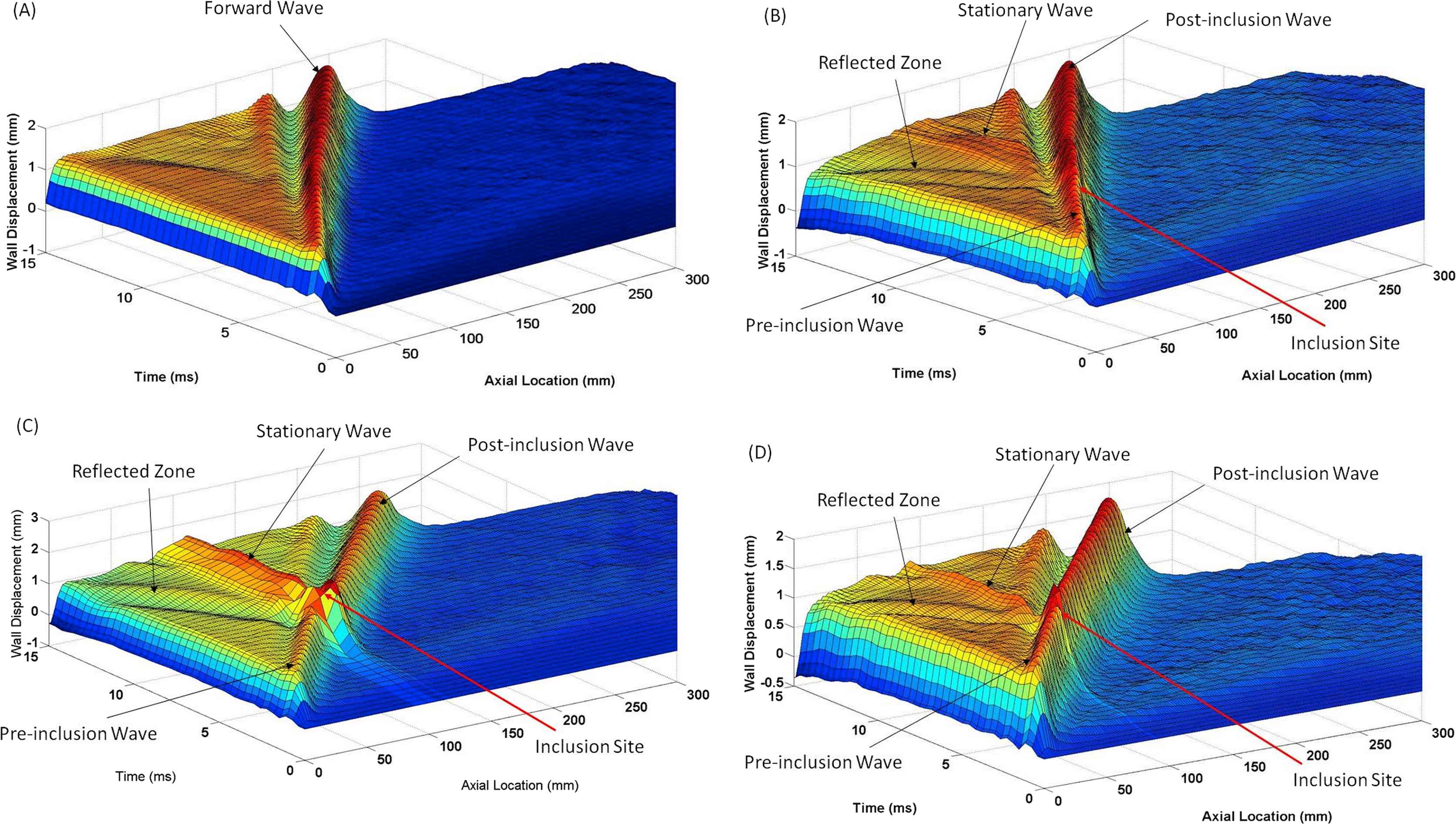
3D waterfall plots of the upper wall displacement for (A) homogenous wall, as well as three representative instances of inhomogeneous walls-(B) Four (N = 4) 2 mm inclusions (S = 2 mm) with modulus E = 3.413 MPa, (C) N = 1, S = 10 mm, E = 3.413 MPa, (D) N = 1, S = 2 mm, E = 2.56 MPa.
Effect of the number of inclusions
Figure 4A–E illustrate the 2D spatio-temporal maps of displacement for the walls (Ew = 5.12 MPa) containing N = 0 (homogeneous), 1, 2, 3, and 4 inclusions, respectively, of size S = 2 mm (10 mm apart) with MC = 1.5−1 (Ei = 3.413 MPa). The results show that increasing the number of inclusions makes the reflection pattern changing from a clear single reflection wave for N = 1 inclusion to a disordered reflection zone for multiple inclusions (N > 1). Additionally, the width of the standing wave grows by increasing the number of inclusions. The width of the standing wave was measured at the largest distance. The effects of numbers of inclusion were also quantified in terms of the width of the standing wave, the PWV of the forward wave and its linear correlation coefficient (r2), as shown in Fig. 7A, D, G, respectively.
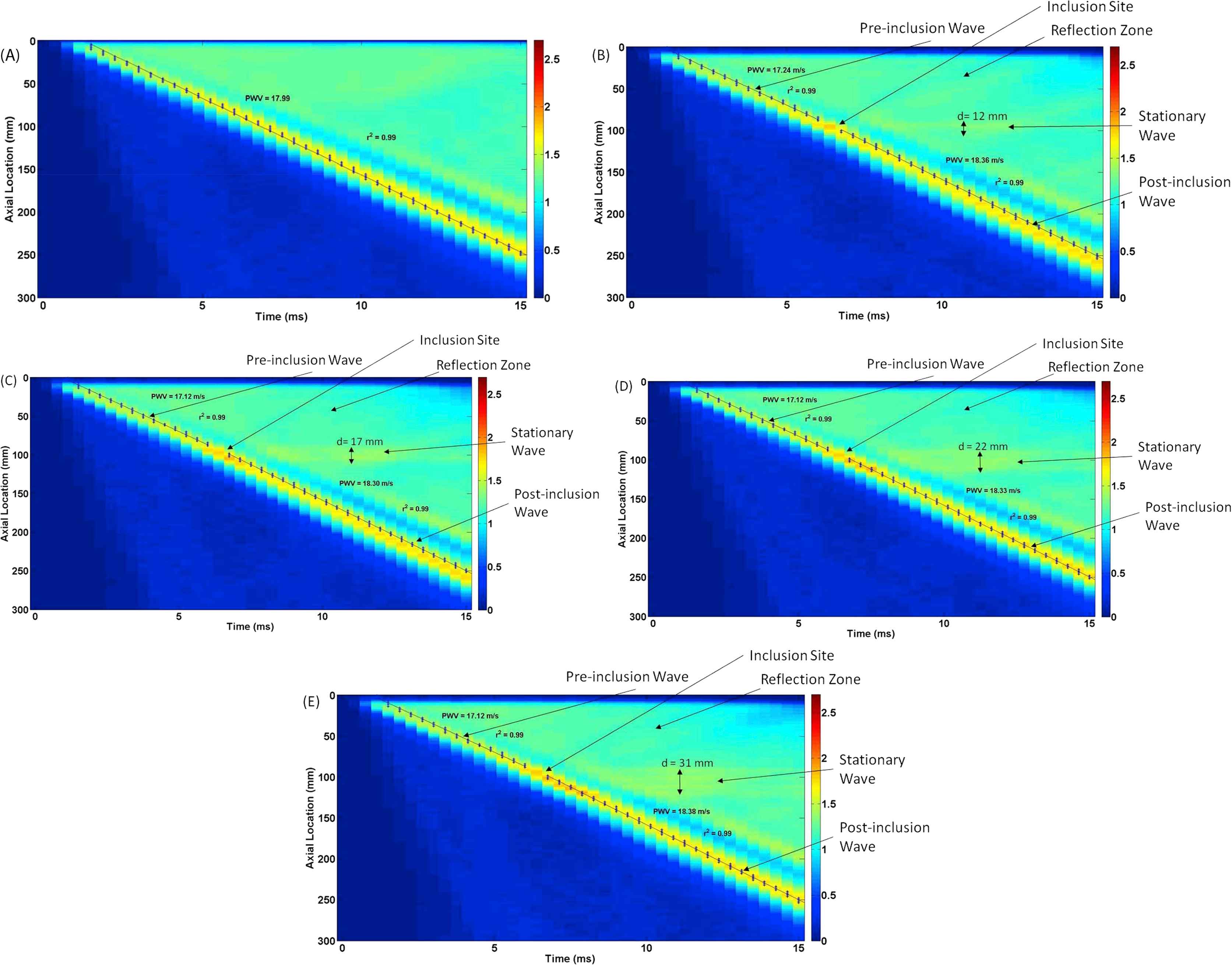
Effects of the number of inclusions (N): Wall displacement 2D spatio-temporal maps for walls (Ew = 5.12 MPa) containing (A) N = 0 (homogeneous), (B) N = 1, (C) N = 2, (D) N = 3, and (E) N = 4 number of inclusions of size S = 2 mm and modulus E = 3.413 MPa.
Effect of the inclusion size
Figure 5A–D illustrate the displacement spatio-temporal maps for walls (Ew = 5.12 MPa) containing no inclusion (homogenous), as well as one inclusion (N = 1) of size S = 2, 5, and 10 mm, respectively, with MC = 1.5−1 (Ei = 3.413 MPa), in order to examine the effect of the inclusion size on the wave propagation. For all different inclusion sizes, there is only one main reflection wave observed which becomes more visible with the increase of the inclusion size. The width and magnitude of the standing wave were also found to grow with the inclusion size increase. The effects of inclusion size were quantified in terms of the width of the standing wave, the PWV of the forward wave and its linear correlation coefficient (r2), as seen in Fig. 7B, E, H, respectively.
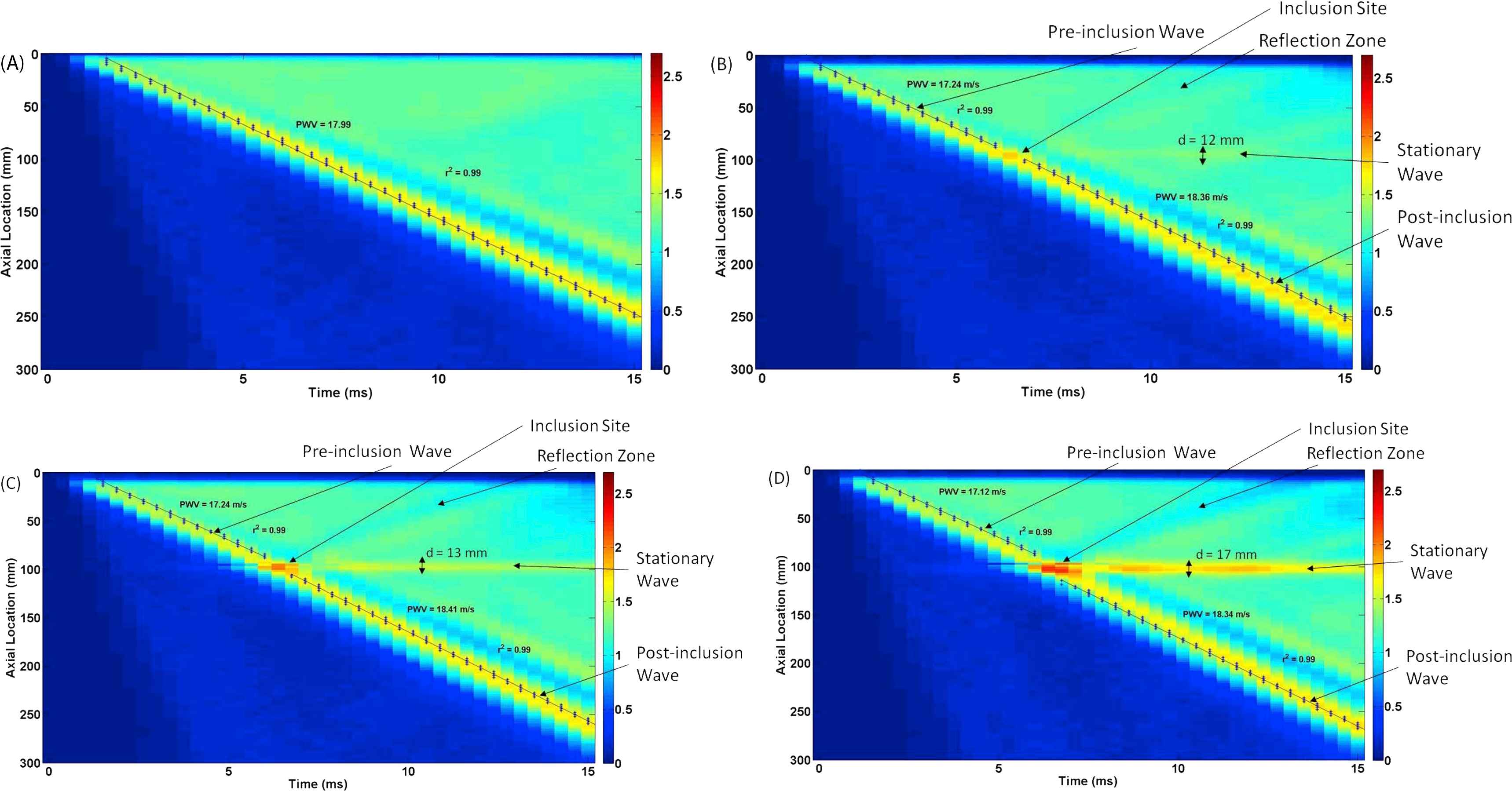
Effects of the inclusion size (S): Wall displacement 2D spatio-temporal maps for walls (Ew = 5.12 MPa) containing (A) no inclusion (S = 0 mm; homogenous), (B) S = 2 mm inclusion, (C) S = 5 mm inclusion, and (D) S = 10 mm inclusion.
Effects of inclusion modulus contrast
Figure 6A–E illustrate the displacement spatio-temporal maps for walls (Ew = 5.12 MPa) containing no inclusion (homogenous), as well as one inclusion (N = 1) of size S = 2 mm, with modulus contrasts of MC = 1.25−1 (Ei = 4.10 MPa), 1.5−1 (Ei = 3.413 MPa), 1.75−1 (Ei = 2.93 MPa), and 2−1 (Ei = 2.56 MPa), respectively. The results show that there is only one clear main reflection wave for all modulus contrasts, which becomes more apparent with the decrease of the modulus contrast. The width of the standing wave decreases as the inclusion modulus contrast does so. The effects of inclusion-to-wall modulus contrasts were quantified in terms of the width of the standing wave, the PWV of the forward wave, and its linear correlation coefficient (r2), as shown in Fig. 7C, F, I, respectively.
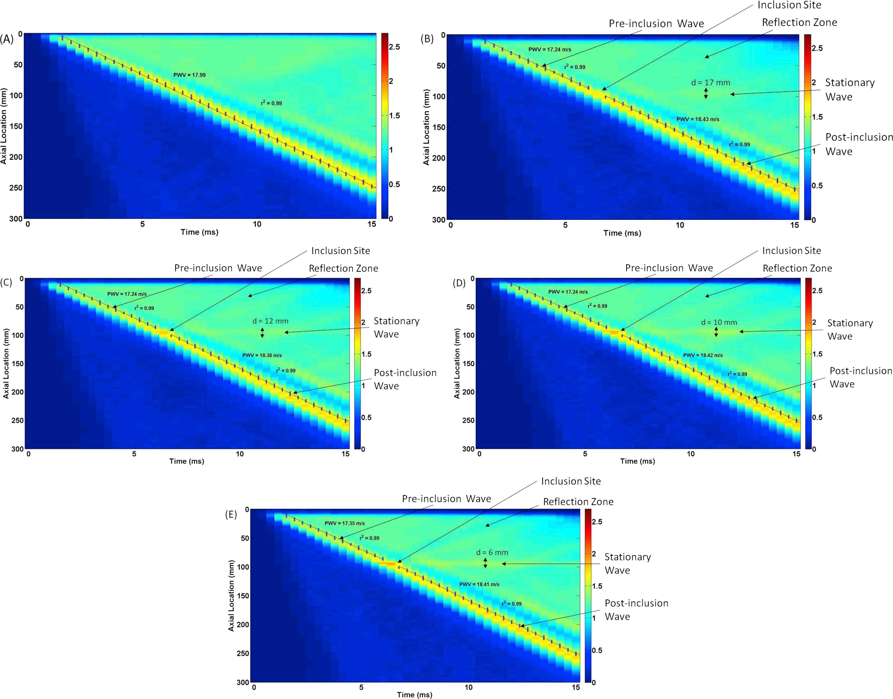
Effects of inclusion-to-wall modulus contrast: Wall displacement 2D spatio-temporal maps for walls (Ew = 5.12 MPa) containing (A) no inclusion (MC = 1), as well as N = 1 inclusion of S = 2 mm, with modulus contrast of (B) MC = 1.25−1 (Ei = 4.10 MPa), (C) 1.5−1 (Ei = 3.413 MPa), (D) 1.75−1 (Ei = 2.93 MPa), and (E) 2−1 (Ei = 2.56 MPa).
Quantified parameters
Figure 7 shows the quantified findings on the effects of number of inclusions (N), inclusion size (S), and inclusion modulus contrast (MC) on the width of the standing wave (d), pulse wave velocity (PWV) of the pre- and post-inclusion forward waves, and the relevant linear correlation coefficient (r2). It is seen that the width of the standing wave has a linear correlation to the number of inclusions and inclusion modulus contrast, Fig. 7A and B, respectively, but a lower correlation for inclusion size, Fig. 7C. The PWVs were measured on the pre- and post-inclusion forward waves (Fig. 7D–F). The post-inclusion PWVs were seen to be higher than the pre-inclusion PWVs for all three categories. The PWV measurements consistently increase as a result to changes in the inclusion properties. The r2 of the PWVs in all three categories, Fig. 7G–I, are found not to yield significant change, and stay high (≈ 0.99). It also indicates that tracking the waves based on the 80% foot definition has been an appropriate choice in reliably measuring PWVs.
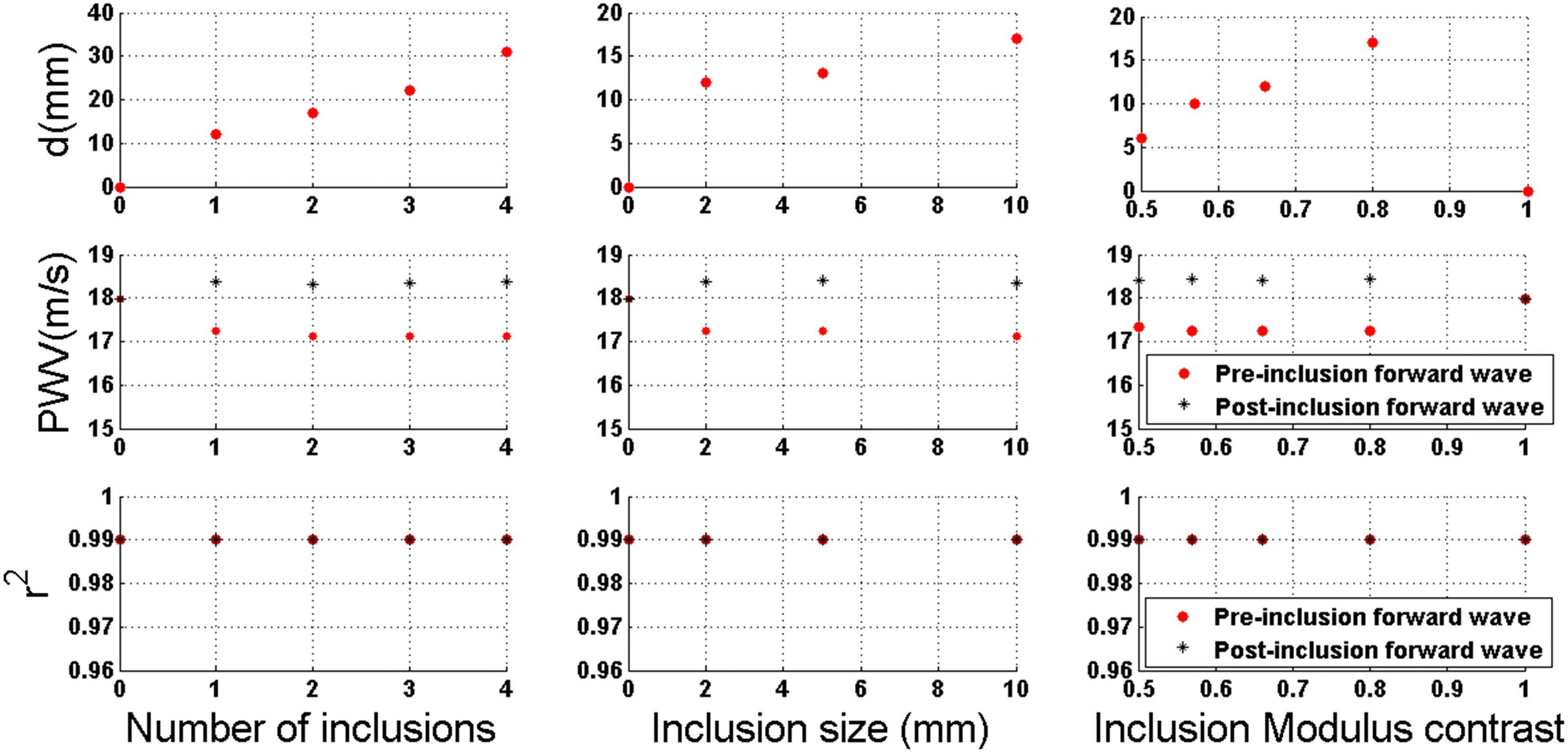
Quantified effects of the numbers of the inclusion (N), inclusion size (S), and inclusion-to-wall modulus contrast (MC) on the wave propagation characteristics.
Discussions and conclusion
Currently, the aortic PWV is measured globally by estimating an average velocity with measurements at two locations: the carotid and femoral arteries.11,16 This accuracy of such global-PWV-based methods can be deteriorated due to the lack of knowledge of the arterial precise geometry, assuming that it is of a single longitudinal flow, and the absence of obtaining a regional PWV along a vascular branch.11,19 Furthermore, majority of cardiovascular diseases have shown to entail focal arterial wall degradations,21–23 which may not be detected based on a global-PWV-based method.
Feasibility of using numerical methods such as FSI simulations to generate pulse wave propagations in simple geometry modeled arteries and determine local PWVs has been established.35 Furthermore, studies to determine the effects of various hard inclusions on the arterial wall and its outcome on the wave propagation in order to establish quantitatively and qualitatively markers to capture these differences have been found.36 The aim of this study is to examine the effects of various soft inclusions on the pulse propagation in order to further establish confirmation that qualitative and quantitative markers can be used to characterize properties such as number of inclusions, inclusion size, and modulus.
Based on the simulation results, it was determined that the quantitative and qualitative markers on the wall displacement spatio-temporal maps can be properly used to make assumptions on the properties of the wall inclusions and to differentiate between the changes in inclusion numbers, size, and modulus. Figure 4A–E shows that forward propagation were affected by inclusion numbers similar to the hard inclusion study36 where there were pre- and post-inclusion propagations with different velocities. Also, as was found in the hard inclusion study, the difference in pre- and post-inclusion forward PWVs was not significant as there is only about a 6% difference between them. The standing wave created by the inclusions did increase in diameter as inclusion number increased. This coincides with the same findings for hard inclusions. Standing wave diameter is the most evident marker to detect increase in the number of inclusions. Figure 5A–D shows several distinct observations found when comparing inclusion size models. The stationary wave diameter increases as the inclusion size increases which is also found in the hard inclusion study.36 The change in diameter is not substantial when compared among different models. There is only about an 8% change between 2 and 5 mm inclusion model. Also, unlike that in the hard inclusion study, the magnitude of the stationary wave increases here as the inclusion size does, and therefore, the stationary wave displacement can be an effective marker when detecting inclusion size for soft inclusion models. Lastly, the PWV gets disrupted at the inclusion site which is also found in the hard inclusion study resulting in pre- and post-inclusion propagation velocities. This disruption does not create much of a difference in the pre- and post-inclusion PWVs as there is only about a 6% change between models. Figure 6A–E shows that forward propagation were affected by the inclusion modulus. This is similar to the hard inclusion study36 as both pre- and post-inclusion propagations had different velocities. Similar to the previous results, the change in velocities was not substantial since there is about a 6% different between pre- and post-inclusion forward PWVs. Comparable to the hard inclusion study, the standing wave created by the inclusions did decrease in diameter as the soft inclusion modulus decreased. The overall results suggest that the standing wave diameter may be the most evident marker to detect increase or decrease in the inclusion modulus. When comparing quantifiable parameters, the results in this study are shown to be as reliable as the hard inclusion study.36 Figure 7 shows the three parameters measured: standing wave diameter, PWV, and r2. Standing wave diameters show good linear correlation for number of inclusions but less for inclusion size and none for inclusion modulus. The hard inclusion study36 shows good correlation in all three categories. Also, both studies show stability of the pre- and post-inclusion forward PWVs over inclusion size, numbers, or modulus in addition to a similar separation in velocities. Lastly, both studies show strong r2s in all three categories confirming method to calculate PWVs deemed appropriate.
The results presented here support the previous works on examining the effects of arterial wall inhomogeneities on the wave propagation, and establish quantitative and qualitative markers to infer on the properties of the nature of the inhomogeneities. The modeling parameters, including those on wall material properties, fluid properties and geometry, were chosen in accordance to other numerical and experimental studies,30,31,35,36 primarily to serve the purpose of establishing the relationship between the wave dynamics and the wall inhomogeneities; an essential part of which is to have strong, fully-detectable wall displacements on the forward and –usually weaker– reflected waves. The findings reported here and along with the information on hard inclusions combined can eventually be used to analyze the simulation results on pathological and patient-specific geometries and wall inhomogeneities such as those seen on atherosclerotic and aneurysmal blood vessels, for which both softening and hardening of the walls have been reported.42–45 More importantly, once the fundamental baselines for wall irregularity-wave dynamic relationships are fully understood on patient-specific simulations and are validated against experimental phantoms, they can be used in reverse direction, serving as templates to better interpret noninvasive medical images, in order to infer more conclusions on the possible irregularities on diseased aortas. It should be kept in mind that the absolute values of the arterial wall stiffness might not be as important for diagnosis purposes as the relative changes in the local stiffness are. Once the spatio-temporal maps of the wall displacements are obtained in vivo, the benchmark results provided in the present study can be used to identify similar biomarkers on the map, and to relate them to the associated types of stiffness changes. Future studies are needed to further investigate the wall irregularity-wave dynamic relationships under in vivo conditions, and to enhance the understanding of clinical implications of PWI in early detection of disease developments, where changes in the material properties are expected to proceed those in geometrical properties.
Conflict of interest
There is no conflict of interest in this study to disclose.
Acknowledgments
The authors would like to thank the Department of Mechanical Engineering at Stevens Institute of Technology for administrative and financial support throughout the conduct of this study. We would also like to extend our gratitude to SIMULIA Academic Support at Dassault Systèmes for their technical advices.
References
Cite this article
TY  - JOUR
AU  - Igor Inga
AU  - Danial Shahmirzadi
PY  - 2015
DA  - 2015/05/15
TI  - In silico characterization of the effects of size, distribution, and modulus contrast of aortic focal softening on pulse wave propagations
JO  - Artery Research
SP  - 10
EP  - 18
VL  - 11
IS  - C
SN  - 1876-4401
UR  - https://doi.org/10.1016/j.artres.2015.04.002
DO  - 10.1016/j.artres.2015.04.002
ID  - Inga2015
ER  -