
Enhancing coronary Wave Intensity Analysis robustness by high order central finite differences
- DOI
- 10.1016/j.artres.2014.03.001How to use a DOI?
- Keywords
- Coronary artery disease; Sensitivity analysis; Wave Intensity Analysis
- Abstract
Background: Coronary Wave Intensity Analysis (cWIA) is a technique capable of separating the effects of proximal arterial haemodynamics from cardiac mechanics. Studies have identified WIA-derived indices that are closely correlated with several disease processes and predictive of functional recovery following myocardial infarction. The cWIA clinical application has, however, been limited by technical challenges including a lack of standardization across different studies and the derived indices’ sensitivity to the processing parameters. Specifically, a critical step in WIA is the noise removal for evaluation of derivatives of the acquired signals, typically performed by applying a Savitzky–Golay filter, to reduce the high frequency acquisition noise.
Methods: The impact of the filter parameter selection on cWIA output, and on the derived clinical metrics (integral areas and peaks of the major waves), is first analysed. The sensitivity analysis is performed either by using the filter as a differentiator to calculate the signals’ time derivative or by applying the filter to smooth the ensemble-averaged waveforms.
Furthermore, the power-spectrum of the ensemble-averaged waveforms contains little high-frequency components, which motivated us to propose an alternative approach to compute the time derivatives of the acquired waveforms using a central finite difference scheme.
Results and Conclusion: The cWIA output and consequently the derived clinical metrics are significantly affected by the filter parameters, irrespective of its use as a smoothing filter or a differentiator. The proposed approach is parameter-free and, when applied to the 10 in-vivo human datasets and the 50 in-vivo animal datasets, enhances the cWIA robustness by significantly reducing the outcome variability (by 60%).
- Copyright
- © 2014 Association for Research into Arterial Structure and Physiology. Published by Elsevier B.V.
- Open Access
- This is an open access article distributed under the CC BY-NC 4.0 license (http://creativecommons.org/licenses/by-nc/4.0/).
Introduction
Two decades following its introduction, Wave Intensity Analysis has become an established technique to examine arterial dynamics.1,2 Improvements in catheters3,4 in the past decades have enabled the application of Wave Intensity Analysis in the coronary arteries,5–8 which is the focus of this paper. The goal of recent investigations was aimed at exploiting the capacity of coronary Wave Intensity Analysis (cWIA) to distinguish between the proximal haemodynamics and the impact of cardiac mechanics on the microcirculation, for clinical translation. More specifically, the Backward Expansion Wave (BEW) has been primarily studied in order to elucidate the link between myocardial relaxation and the sharp diastolic rise of coronary inflow.
However, application of WIA to the coronary vessels has been considered with skepticism from some investigators9 mainly due to the lack of evidence that the cWIA-derived indices can have prognostic value. Moreover, the high dependency of the cWIA outcome on the practitioners, mainly due to the unknown dependency on the noise introduced by the acquisition process and the pre-processing filtering step, has been considered a notable weakness. While the first point has been recently addressed since the clinical usefulness of cWIA and the prognostic value of the cWIA derived metrics have been consistently demonstrated,10–12 the second one remains still unknown. This is a major motivation to undertake the current study in order to enhance the robustness of the cWIA outcome.
In a recent study Kyriacou et al.10 used cWIA to identify the optimal atrioventricular delay in biventricular pacing in order to improve ventricular contractility and relaxation thereby increasing the cardiac output. Lockie et al.11 found that a cWIA-derived index was central in the commonly seen but poorly understood phenomenon of ‘warm-up’ angina. Most recently, De Silva et al.12 have shown for the first time that a real-time derived BEW peak can predict functional myocardial recovery following myocardial infarction. Given these successes it is becoming increasingly relevant to assess the robustness of cWIA outcomes independently of clinical context through each of the steps involved in the analysis.
In general, measured arterial pressure and velocity waveforms contain appreciable levels of noise. In the coronary vessels this situation is further exacerbated by cardiac motion. For this reason, in the literature, pressure and velocity signals are typically ensemble-averaged and subsequently smoothed most often by using the Savitzky–Golay (S–G) filter.1,5,11–14 This filter is applied because it is believed to preserve the peaks of the waveforms, which are a principal feature in performing a reliable cWIA.
However, note that the quantities involved in the cWIA are exclusively the first order time derivatives of the signals, on which the relative impact of smoothing is greater than on the signals themselves. Surprisingly, the influence that the S–G filter parameters have on the signals’ time derivative and in turn on the cWIA profile has not been investigated to date. Furthermore, the values of the filter parameters used in the different studies are almost never included in the publications.1,5,11,12,14
Therefore, the purpose of this paper is firstly to qualitatively and quantitatively characterize the impact that the S–G filter parameters have on the cWIA outcome and the derived clinical metrics.
The S–G filter is applied as a differentiator to calculate the signals’ time derivative, input of the cWIA, directly from the ensemble-averaged waveforms. However, there is an alternative approach employed in the literature,5,11 which is to compute the signals’ time derivative after smoothing the ensemble-averaged signals. Due to the lack of a preferred or standardized approach in the literature, we performed the sensitivity analysis for both approaches.
In addition, with the purpose of introducing a straightforward standardized parameter-free approach, we propose a new procedure that applies a finite difference scheme to estimate the time derivatives directly from ensemble-averaged data. We then compare the S–G approaches with the proposed procedure in terms of the variability exhibited with respect to the cWIA metrics (Pulse Wave Speed, area and peak of the main waves and the total energy carried by the forward and backward travelling waves).
Methods
Study protocol and data acquisition
Retrospective human data: method development
The proposed method for cWIA was developed using 20 recordings from 10 human subjects scheduled for coronary angiography or percutaneous coronary intervention. Patients had given informed consent to take part in the study approved by local ethics committee. Data acquisition was as per routine clinical protocols employed in the hospital.3
Prospective animal data: method validation
The developed method for cWIA was prospectively applied to intracoronary recordings from 40 kg Danish Landrace Pigs (Skejby University Hospital, Aarhus, Denmark). The studies were conducted with the approval of the local ethics committee. All experiments were performed in compliance with the World Medical Association Declaration of Helsinki regarding ethical conduct of research involving animals. On anaesthetized, mechanically-ventilated animals, a left lateral mini-thoracotomy was performed and an external balloon constrictor was placed around the proximal Left Anterior Descending coronary artery (LAD). External circumferential constriction was controlled via a closed airtight system by inflating air volumes, via a plastic externalized tube, connected to a manometer and air-filled Luer Lock syringe. The chest was then sutured.
Peripheral artery access was via a cut-down to the right femoral artery. A 6F sheath was introduced using a Seldinger technique. 6F guide catheter was advanced to the ascending aorta under fluoroscopic guidance. Intra-arterial unfractionated heparin (70 units/kg) was administered. A dual pressure and Doppler sensor (Combowire, Volcano Corp) and single pressure sensor Primewire (Volcano Corp) were connected to the Combomap (Volcano Corp) and advanced to the tip of the guiding catheter. The pressure signals were then normalized. The Combowire was advanced to the distal LAD and Primewire positioned at the tip of the guide catheter in the left main stem to provide proximal pressure recording. The Combowire was manipulated to optimize the Doppler trace. Continuous Doppler and pressure recordings were made. The external balloon constrictor was then inflated to create coronary stenoses of varying severity. The coronary constrictions were graded to reproduce coronary artery stenoses ranging from 0.75 to 0.3 FFR. Intracoronary nitroglycerine (300–500 μg) was given to reduce the effects of coronary spasm on the measured parameters. Once the distal pressure became stable, resting measurements were taken. Intracoronary adenosine (48–96 μg) was then administered to cause maximal hyperaemia. From these data a standard set of parameters for coronary stenosis severity and microvascular function (Fractional Flow Reserve, Hyperemic Stenosis Resistance, Coronary Flow Reserve, Hyperemic Microvascular Resistance) was calculated in real-time. Intracoronary adenosine achieves maximal hyperaemia within 6–8 s, after which the constrictor balloon is deflated.
All signals were sampled at 200 Hz and stored for off-line analysis. The data were imported into the custom software (Studymanager, Academic Medical Center, University of Amsterdam, The Netherlands) and 10–20 consecutive representative beats were extracted during resting and hyperemic conditions.
In total 64 coronary lesions were created in 8 animals. All data were collected and analysed irrespective of data quality. For ease of comparison and subsequent implementation of the developed method, the animal protocol, as far as possible, mirrored the human clinical routine used to measure intracoronary haemodynamics.3
Wave Intensity Analysis
Following the in-depth overview provided by Parker1 the main steps involved in the WIA are presented. Briefly, the beats of interest are selected and then pressure and velocity waveforms are ensemble-averaged in order to remove high frequency noise. To compute the resulting signals’ time derivative, input to the WIA, two approaches can be pursued. First, the standard approach is to take advantage of the Savitzky–Golay differentiating filter to compute the derivative directly from the ensemble-averaged signals, as highlighted in the original publication.13 This approach is indicated as SG-D in the paper. Secondly, the ensemble-averaged waveforms can be smoothed first using a Savitzky–Golay smoothing filter and then the time increments of the smoothed pressure p(t) and velocity v(t) signals computed:
This second approach is indicated SG-S in the paper. It represents an alternative method sometimes employed in the literature.5,11
After computing the signals’ time derivative (using Eq. (1) or applying S–G as a differentiator), it is possible to calculate the Wave Intensity:
Dividing the time increments by dt avoids the WIA dependence to the sampling time.15
The fundamental property of Wave Intensity, from Eq. (2), is that at each sampling point of the measured waveforms the sign of dI(t) highlights if forward (+) or backward (−) travelling waves are dominant. With a further assumption that forward and backward travelling waves sum linearly when interacting, the simultaneous forward and backward travelling waves can be separated, as follows:
The PWS is estimated by using the sum-of-squares method16,17
Savitzky–golay filter sensitivity analysis
The Savitzky–Golay filter performs a least squares regression in moving windows. Specifically, for each group of points, a polynomial function of degree N is fitted using least-squares to the M points in the sampling window. Therefore, N and M represent the tunable parameters for the filter.
Initially, we chose a dataset with good quality pressure and velocity signals (Fig. 1(a)) representing a dataset of close-to-ideal quality obtainable in a clinical setting. After ensemble-averaging 9 consecutive beats, the velocity signal time derivative has been calculated using the S–G filter as a differentiator with a second order polynomial degree (N = 2) and varying window width from 3 to 15 in steps of 4. We then repeated the SG-D approach increasing polynomial order N = 3,4,5 while varying accordingly the corresponding window width ranges M = [5–17], [5–17], [7–19], maintaining the step size of 4. The reason behind the choice of these window widths is provided in the next section. This step size of 4 was chosen since for the S–G filter the window width has to be an odd number. The initial value of M for each range was increased since for the S–G filter M > N+1. The pressure waveform has been ensemble averaged but left unsmoothed.
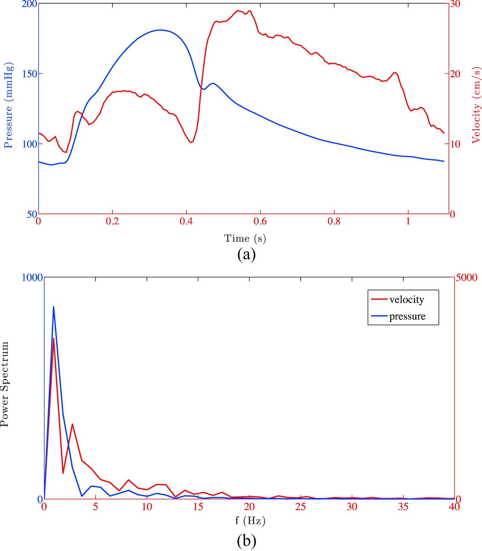
Pressure and velocity ensemble-averaged signals are shown in panel (a) along with the power spectrum of the signals in panel (b).
We then performed cWIA following the steps outlined in Wave Intensity Analysis, for every combination of polynomial order and window width range. For each of the obtained cWIA profiles we computed the PWS, the total energy carried by the forward and backward travelling waves and the areas and peaks of the Forward Compression Wave (FCW), the Backward Compression Wave (BCW) and the Backward Expansion Wave (BEW).5
We then repeated the same protocol with the same parameter range but using the S–G filter to smooth the velocity waveform and then compute the velocity time derivative using Eq. (1)
Although in practice the velocity signal tends to contain a greater degree of noise, it may be argued that both the pressure and velocity signals should be smoothed because both quantities are involved in the sum-of-squares method. Therefore, we repeated the same analysis protocol illustrated above for both pressure and velocity signals, for both SG-D and SG-S approaches.
Parameters choice
The S–G filter was initially studied and widely applied in the field of spectrometry where the main filter properties have been described.13,20–23 It has been highlighted that increasing the polynomial order for a fixed window width reduces smoothing and preserves the narrower signal features.20,23 This is the reason to explore the impact of increasing the polynomial order. Conversely, increasing the window width for a chosen polynomial degree intensifies the smoothing on the signal.21,23
The absence of filter parameters reported in the literature complicates the selection of a representative range for a sensitivity analysis. Only Koh et al.24 reported the number of points per sampling window (M = 11) used, but without specifying the polynomial degree chosen. Therefore, we selected a broad range of polynomial degrees and window widths in order to obtain a clear picture of the impact parameter regimes have on the cWIA results, constrained by the two following observations. First, the acquired signals are commonly sampled at 200 Hz providing approximately 200 points per cardiac cycle. Second, the main features in the velocity signal need to be preserved over a range of different time scales, spanning from the rapid rise in early diastole to the wider systolic plateau.
The perfect combination of N, M would be the one providing the maximal noise cancellation with the minimal information loss.
Analysis of the Savitzky–Golay filter properties when used as a differentiator (SG-D approach) has revealed22,23 that the key parameter for optimizing the filter is the ratio between the Full Width at Half Maximum (FWHM) of the signal derivative and the window width. In Luo et al.,23 it is shown that for N = 3,4,5,6 the optimal window width to minimize the error in computing the peak of the signal derivative is
Although these error estimates are obtained on analytical functions of Gaussian derivative, which departs somewhat from real data, applying the theoretical results to our case, where the FWHM of the velocity time derivative peak is made up of approximately 10 sampling points, for the ranges of the filter window width M chosen
- •
N = 2; FWHM/M > 0.67;
- •
N = 3,4; FWHM/M > 0.59;
- •
N = 5; FWHM/M > 0.63;
It follows that selected widths of the window are in the parameter range where SG-D filter performs optimally (FWHM/M > 0.4).
Finally, for a signal sampled at 200 Hz, increasing the window width in the range [3–15] in steps of 4 (N = 2) is roughly equivalent to low-pass the filter at 66 Hz, 29 Hz, 18 Hz and 13.5 Hz. Considering the power spectrum of the signals (Fig. 1(b)) it is clear that most of the information belongs to frequencies lower than 13 Hz (88% for the velocity and 95% for the pressure). In conclusion, particular care was taken to ensure the range of parameters selected for the SG-D filter evaluation is confined to within its optimal operating range.
Central finite difference
As pointed out in the Introduction, it is paramount to move towards a standardization of each of the steps involved in cWIA with the final goal of clinical translation. Therefore, a method stable and parameter-free is greatly preferred. The simplest choice is to enhance the signals’ time derivative estimation by high order finite differencing, since for cWIA the accurate calculation of the time derivative of the signals is fundamental. For this reason, in this study, the pressure and velocity derivatives were calculated directly from ensemble-averaged data using a central finite difference scheme. This means that in order to compute the time derivative of a function f at a point xi, only pairs of points (on either side) are used. For instance, the first derivative of f, with a spacing h
| Order of accuracy | xi−4 | xi−3 | xi−2 | xi−1 | xi | xi+1 | xi+2 | xi+3 | xi+4 |
|---|---|---|---|---|---|---|---|---|---|
| 2 |
|
|
|||||||
| 4 |
|
|
|
|
|||||
| 6 |
|
|
|
|
|
|
|||
| 8 |
|
|
|
|
|
|
|
|
Central finite difference coefficients for the first derivative along with their accuracy order.
When considering the boundary treatment at the start/end of the time signal, we applied a progressively decreasing order schemes that requires fewer points.
Central finite difference sensitivity analysis
The pressure and velocity time derivatives exhibit sharp variations due to the rapid changes observable for example in early diastole in the velocity profile and the dicrotic notch in the pressure waveform. Consequently, the number of points necessary to properly approximate the time derivative, driving the choice of the scheme order, has to be a compromise with respect to the width of different features within the signal.21 Increasing the number of points per window beyond 8, would have combined points belonging to different features, affecting the peaks of the time derivatives thereby influencing the cWIA indices.
Using the same dataset as in Parameters choice, we computed the time derivative of the pressure and velocity waveform applying the central finite difference scheme from 2nd to 8th order directly from ensemble averaged data. This method is labelled CD in the paper. For each order we then computed the cWIA profile and the derived metrics, mirroring the procedure followed when SG-D or SG-S are applied.
Comparison
The comparison between each polynomial order for the SG-D approach, the SG-S approach and the CD approach was made in terms of the variability exhibited in the estimated PWS and the cWIA-derived metrics, as the window width (M) or the finite difference order is increased. In the absence of a standard index for S–G variability, given a range of window widths M = [M1,…,Mend] for a fixed polynomial order N, the variability is defined as
Validation
After concluding the analysis on the in-vivo human dataset, we repeated the same study on 50 in-vivo animal datasets, spanning over a variety of signal quality and stenosis severity, determined using the FFR index.25 This enabled us to evaluate the observations made from the in-vivo human dataset analysis. We compared both the S–G approaches, smoothing both the pressure and velocity signals, for N = 2,4 and M = [3–15], [5–17] in steps of 4 with the CD approach, with the order between 2nd and 8th.
For comparison metrics only the FCW and BCW have been considered. This is due to the fact that the BCW is predominant over the BEW in these datasets, where external occluders were used on the LAD. In addition to these metrics, we also computed the ratio between the total area under the backward- and forward-travelling waves (B/F). The B/F value was observed to be around unity for healthy vessels and can reach a value of 2 in the presence of stenosis.14
Results
For ease of comparison, in this section we present the results not in the order specified in the Methods but based on each metric with the sensitivity of the S–G approaches grouped together with the central finite difference results.
Impact on the velocity waveform
Increasing the window width for the polynomial order N = 2 has a minimal effect on the velocity profile, however it has a significant impact on its time derivative for both SG-D and SG-S methods, as clearly visible in Fig. 2(a)–(c). On the other hand, increasing the CD order exhibits a more stable behaviour with respect to the time derivative Fig. 2(d).
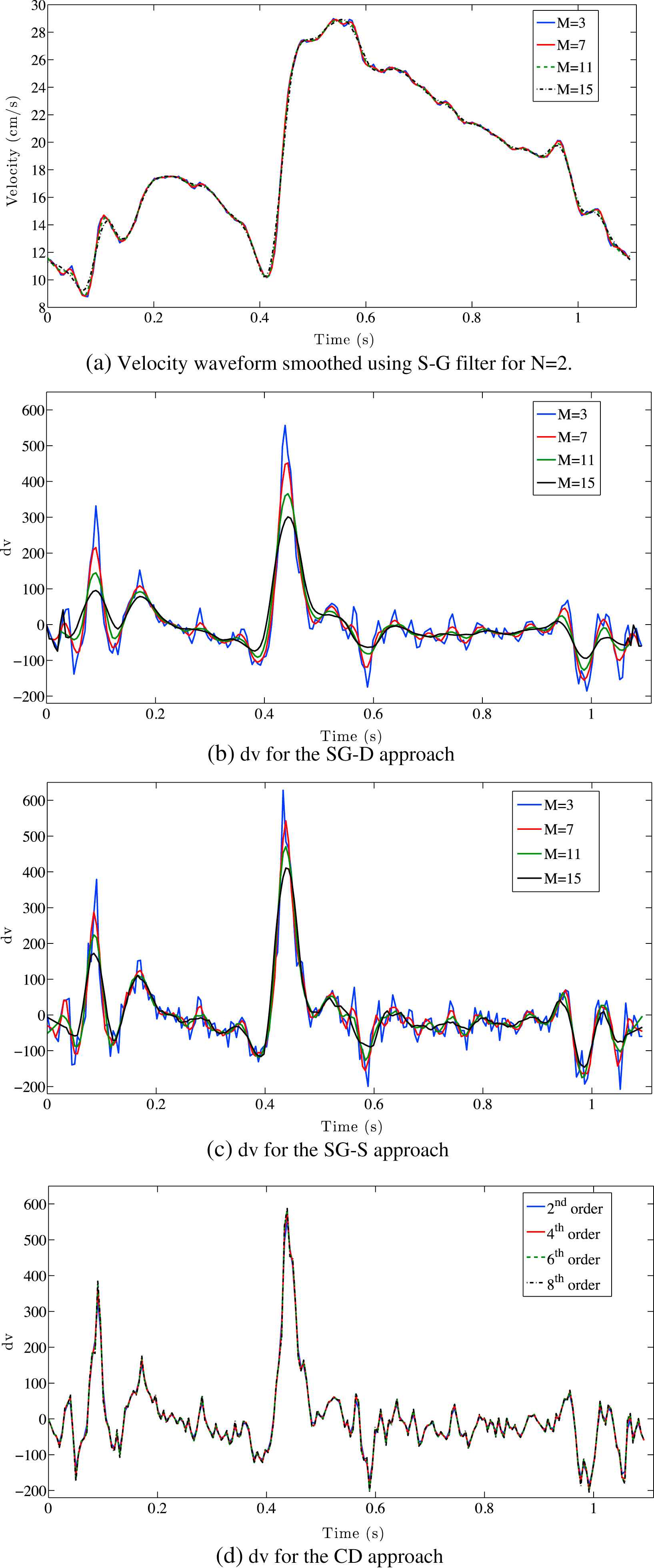
a) The effect of the smoothing (N = 2; M = 3,11,15) on the velocity waveform is limited. (b,c) The impact of varying the filter width on the time derivative for the SG-D approach and the SG-S one severely impact on the velocity time derivative peak. (d) Varying the central finite difference order provides more stable approximation of the time derivative.
Wave Intensity profile
Using either SG-D or SG-S, varying the window size for N = 2 has a strong impact on the cWIA profile significantly flattening all main waves (Fig. 3(a) and (b)). This is the consequence of the S–G smoothing and the SG-D differentiator effects on the time derivative highlighted above. The cWIA profile obtained applying the CD approach is only slightly affected by the order of the scheme (Fig. 3(c)).
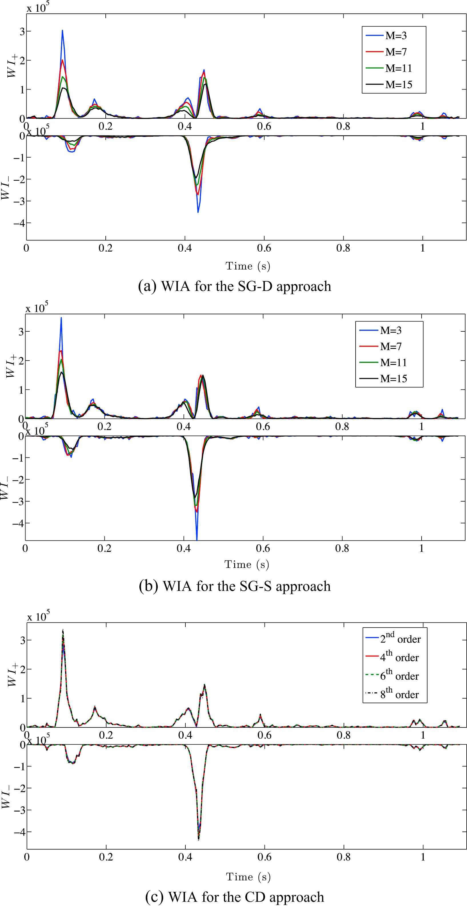
Wave Intensity Analysis separation into forward travelling waves (top) and backward travelling waves (bottom) is displayed, using the SG-D approach (a), the SG-S approach (b) (N = 2, M = [3, 15]) and the central finite difference one (c). The significant flattening of the main waves caused by the increase of smoothing (a–b) introduced is clearly visible. The WI± units are W m−2 s−2.
Pulse Wave Speed
The PWS is consistently overestimated when the window width is increased. The estimated PWS increases by 45% and 20% between window width M = 3 and M = 15 for the SG-D approach and the SG-S, respectively (Table 2). In contrast, increasing the differencing order from 2nd to 8th produces a variability of 3%. Note that, in the subsequent results, we did not utilise a fixed PWS due to the asymmetrical dependence of WIA on PWS; this is explained further in the Discussion.

The variability for the three different approaches Savitzky–Golay smoothing (SG-S), Savitzky–Golay differentiator (SG-D) and Central Finite Differences (CD), for the human dataset, are showed. The variability is calculated as percent variation in the examined metrics between the first and last value of the filter window width/finite difference order. In red the combination of parameters which produce significant variability for the S–G approaches are highlighted.
Area under the main waves
As expected from the cWIA profile flattening pointed out above, when the window width is increased the total energy carried by the forward travelling waves varies by up to 34% and 17% for the SG-D approach and the SG-S respectively (Table 2). For the backward travelling waves the variability was 28% and 17% for the SG-D approach and the SG-S.
The CD approach reduces the variability to 5%.
Focusing on the main waves’ areas, increasing M between 3 and 15 causes a variation of 34%, 50% and 17% for the FCW, BCW and BEW respectively for the SG-D approach. The SG-S approach exhibits a variability of 18%, 30% and 8%, respectively. The corresponding figures for the new approach are 5%, 8% and 2%.
FCW, BEW and BCW peaks
The cWIA flattening caused by the increase in M severely impacts on the peak values of waves. For the SG-D approach, the FCW, BCW and BEW peaks vary by 65%, 65% and 45%, for N = 2, when M is increased form 3 to 15. The figures for the SG-S approach are 70%, 36% and 42%, respectively. The CD approach reduces the variability to 19%, 5% and 8% respectively increasing from 2nd to 8th order.
Pressure and velocity separated components
When the pressure and velocity waveforms are separated into forward and backward components, the overestimation caused by increasing the window width for the S–G approach becomes clear (Fig. 4(a) and (b)). Similar results are obtained for the SG-D approach. On the other hand, the separated components for the different finite differencing orders are almost superimposed (Fig. 4(c) and (d)).
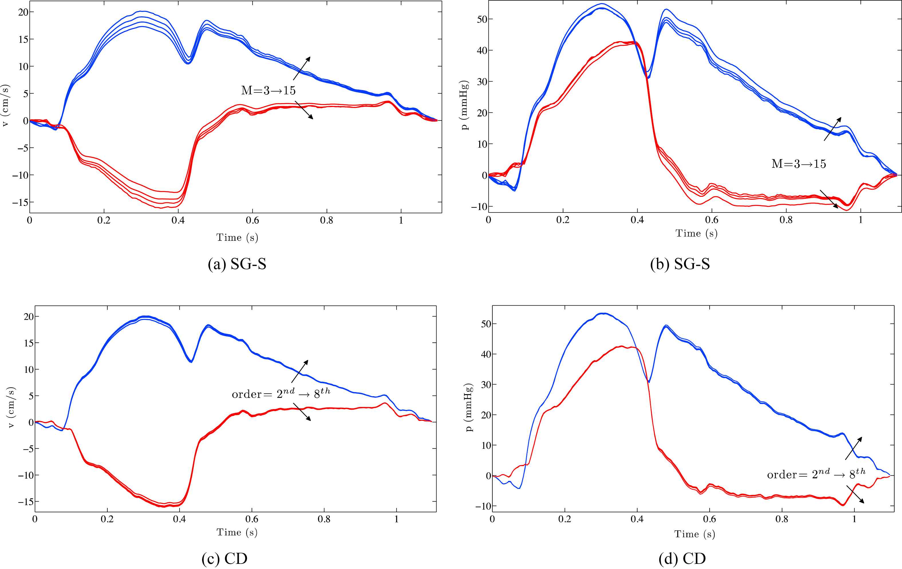
The separated components of pressure and velocity for the SG-S (a,b) and central finite difference approach (c,d) are visualized. The overestimation caused by an increase in smoothing (highlighted by the black arrows) for both the components is clearly visible. For the CD approach the two components are almost superimposed.
Increasing N = 3,4,5
Varying the polynomial order over N = 3,4,5 for the SG-D and the SG-S approach does not seem to significantly improve the variability related to the main waves’ peaks, however, it does provide an enhancement in terms of waves’ areas (Table 2). For the SG-S approach N = 5 performs best, but still exhibiting a variability 3 times higher that the CD approach for the area of the main waves. The variability obtained for N = 4,5 (the best performing) for the SG-S approach remains 2 times higher than the new proposed approach for the FCW, BEW and BCW respectively.
Concerning the total energy carried by the forward and backward waves, for N = 3 the behaviour of the SG-S approach is similar to what was observed for N = 2. Increasing the order to N = 4,5 reduces the variability for the SG-S approach although it still remains 2 times higher than the CD approach. For the SG-D approach N = 5 is still the best performing, but with a variability that is at least twice compared to the new proposed approach. Increasing the polynomial order N reduces the PWS variability for N = 4 up to 10% for both the SG-S and the SG-D approach, however, that still remains significantly higher than the 3% obtained for the new approach.
In conclusion, based on these studies the polynomial degrees N = 5 for the SG-D approach and N = 4,5 for the SG-S approach appear to be the best choice with respect to the variability of the PWS and the wave areas. However, they still exhibit a serious lack of performance when the waves’ peaks are of interest. Repeating the analysis, smoothing both pressure and velocity signals, slightly reduces the PWS variability but increases the variability of the waves’ areas and peaks.
It is possible to argue that the comparison in terms of variability is not completely fair since the values for the window width M chosen for the S–G approaches are larger than the number of points per side of the CD approach. However, the S–G filter width and the central finite difference order cannot be easily related, one being the number of points used to fit a certain order polynomial using least-squares and the other the order after which the Taylor expansion of the function’s derivative is truncated. Moreover, as highlighted in Parameters choice, for a signal sampled at 200 Hz, increasing the window width in the range [3–15] is roughly equivalent to low-pass filter between 66 Hz and 13.5 Hz. Considering that most of the information of the pressure and velocity signals (88% and 95% respectively) belongs to frequencies lower than 13 Hz, it follows that the significant variability exhibited by the S–G approaches is not ascribable to the range of window widths chosen.
Moreover, when we repeated the sensitivity analysis but equalizing the number of points per side between the S–G approaches and the CD method (for instance N = 3, M = 5–9 against 4th–8th order), the results were confirmed. N = 2 it is not an optimal choice even in this case leading to a variability of 10%–20% and 20–30% for the SG-D and the SG-S approach respectively, with respect to the areas under the main waves. The CD method variability range is 3%–8%. Increasing the polynomial order provides an improvement in variability with respect to the main waves’ areas reducing the variability range up to 5%–10%. However, this reduction has to be compared to the CD variability in the range 4th–8th order, which reduces consistently to <1%.
When the peaks of the main waves are considered, both the S–G approaches confirm the lack of performance throughout all the values of N tested. For instance, for the SG-D approach, for N = 5 (the best performing), it is enough to vary M between 7 and 9 to cause a FCW peak reduction of 20%. The CD approach exhibits a variability related to the peaks of 1%–5% when only the orders above the 2nd are considered.
Validation using the animal datasets
The choice of the value for the SG-S filter approach was confined to N = 2,4 because N = 3,5 showed similar performances to the even-order counterparts. We did not extend the validation to the SG-D approach since the results in the human dataset indicated a consistently poor performance.
The results for the animal datasets again confirm the strong overestimation of the PWS when the window width is increased, both for N = 2 (Fig. 5(a)) and N = 4. The CD approach provides a significant improvement in terms of the PWS stability (minimum 59% variability reduction for N = 2, minimum 53% for N = 4). Moreover, the progressive flattening of the cWIA profile caused by increased smoothing (window width) is confirmed from results derived from the entire dataset. The improvement in terms of variability of the CD approach with respect to the SG-S approach for N = 2 is approximately 49%, 56%, for the forward and backward wave energies respectively. For the FCW and BCW the percentages are 54% and 50%.
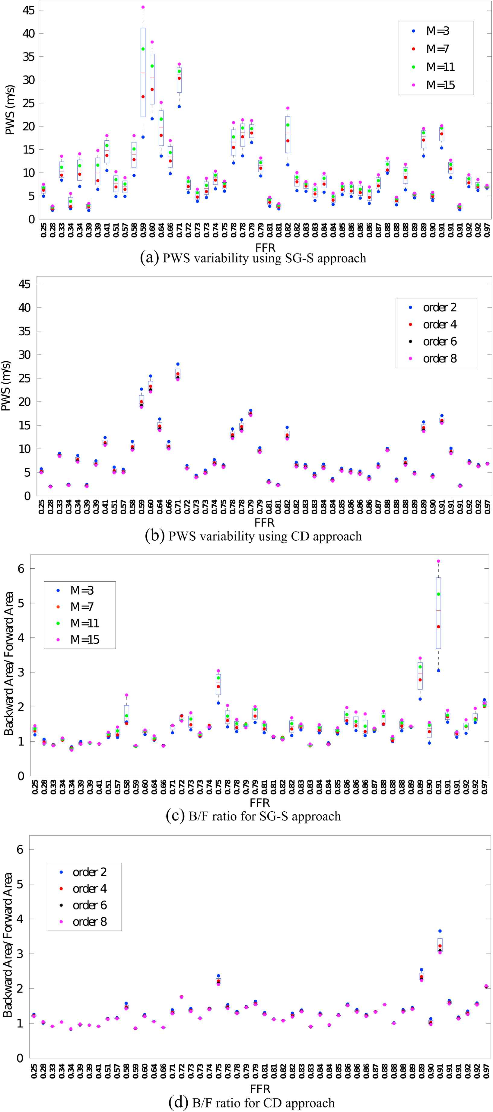
The boxplots for all the analysed datasets are visualised for the SG-S approach for N = 2 (a,c) and for the CD approach (b,d). The significant reduction in variability is remarkable for the estimated PWS (a,b) throughout all datasets analysed. The same reduction is seen with the same magnitude in all the other metrics analysed. The SG-S approach can lead to overestimation of the B/F ratio (c), physiologically expected to be ≈ 1 even if the effect of the smoothing is to underestimate both the forward and backward travelling waves energy. The CD approach provides more physiological values.
For N = 4, the reduction in variability observed is 45%, 34% for the forward and backward travelling waves and 39% and 34% for the FCW and BCW. The minimal reduction in variability provided by the new approach with respect to the BCW and FCW peaks is 16% and 40% respectively. In addition, the variability in the SG-S approach can lead to non-physiological values of the B/F ratio (Fig. 5(c)) whereas the values obtained using the new approach are, barring three exceptions, consistently within the physiological range through all the datasets (Fig. 5(d)). The decrease in variability observed for the B/F using the CD is at least 48% for N = 2 and 45% for N = 4; only one dataset out of the 50 showed greater variability compared to the Savitzky–Golay approach.
Discussion
In this work we have systematically investigated the impact that the S–G filter parameters have on the results of cWIA, both when the filter is used to smooth the ensemble-averaged signals or to directly compute the time derivatives. Although cWIA is gaining clinical relevance, such a sensitivity analysis has not been conducted to date. As discussed below the cWIA profiles and consequently the derived metrics are highly sensitive to the filter parameters, especially when it is utilized as a differentiator. In contrast the method proposed in this study shows significant improvements as demonstrated by the comprehensive evaluation.
Sensitivity of cWIA to S–G filter parameters
We have clearly shown that increasing the smoothing (window width) strongly influences the results of cWIA, leading to a considerable overestimation of the PWS as well as an underestimation of the cWIA derived metrics, over the range of polynomial orders analysed. This result is due to the impact that the S–G filter has on the calculated time derivatives. Increasing the amount of smoothing of the ensemble-averaged waveforms flattens the cWIA profile, through over-damping of the time derivatives. We stress that this impact can be easily underestimated or even missed if the damping effect is gauged directly on the waveforms, rather than their time derivatives. The impact is even stronger when the derivatives are evaluated directly from the S–G filter (SG-D approach), as clearly shown from our analysis.
However, among the wide range of parameters analysed, using a polynomial degree N = 5 for the SG-D approach and N = 4,5 for the SG-S method seems to reduce the variability in both the estimated PWS and the waves’ areas.
When both pressure and velocity signals are smoothed, the variability in the derived metrics increases suggesting that the application of the S–G filter to the pressure waveform should be avoided unless necessary. Interestingly, among the main waves, the BEW is the one that exhibited the least sensitivity to the filter parameters over all values of N and M studied for both the S–G approaches (Table 2). BEW is also the metric that is most commonly reported in the literature.5,10–12,18 We speculate that the importance of the other major waves (FCW, BCW) may have been possibly obscured by the sensitivity of the related metrics to the filtering step. This is also supported by the fact that most of the clinical studies employing cWIA report a post-interventional change in the wave profile of 20–30%, which was found to be within the filter-related variability. However, we stress that these results do not invalidate the previous clinical studies as long as the filter parameters used were consistent for all analysed datasets. Nonetheless, as clearly shown in the S–G sensitivity analysis, changing the filter parameters between analyses of different datasets in the same patient group could possibly lead to erroneous conclusions. Thus, it is of crucial importance to publish the parameters used in any reported analysis to allow a clear comparison between different studies.
It is possible to argue that the PWS should have been kept constant for all cWIA sensitivity analysis to highlight solely the impact of the filter parameters choice. However, as shown in Siebes et al.14 Fig. 2, the WIA profile exhibits an asymmetric dependence on the change in PWS. WIA is not sensitive to a PWS variation of up to 50%, which is over the maximum PWS variation we observed in the sensitivity analysis (Table 2). Moreover, the WIA profile is more sensitive to a reduction than an increase in PWS. In a certain sense, our comparison penalized the CD approach with respect to the S–G approaches, by not assuming a fixed value of the PWS, since varying the finite difference order caused a slight PWS reduction, whereas increasing M increased the estimated PWS.
Finally, that the PWS in the 50 datasets studies have been evaluated using the sum-of-squares method may be perceived as a weakness of the current study, since, it has recently been shown to be inaccurate under a hyperemic regime.9 Even though we are aware of this limitation, we preferred to conduct the sensitivity analysis as well as evaluate the new technique by adhering to the practice used most regularly in the literature. Moreover, it would have been difficult to include the observation19 that the PWS during baseline should be used for the hyperemic state, since we have shown that the PWS value strongly depends on the S–G filter parameters choice.
Performance of the CD approach
To address the variability issue we evaluated central finite differencing of various orders to estimate the time derivative directly from ensemble-averaged data. This new approach, applied to the in-vivo human dataset showed a significant reduction in variability through all the analysed metrics, when compared with the S–G approaches. Moreover, results show that the choice of the differencing order does not have a significant effect on the derived metrics. When applied to the animal datasets, the reduction in variability was considerable with the new approach. It provided a minimum reduction of variability in the PWS of 53%, positive total area of 45%, negative total area of 34%, BCW area of 34%, FCW area of 39%, peak BCW of 16% and peak FCW of 40% compared to the S–G approaches. Furthermore the ratio B/F produces more physiological values using the CD approach when compared to results derived using the S–G filter. These conclusions were derived from evaluating our proposed approach for a wide range of signal qualities and stenosis severities and our technique was shown to be superior in all cases. However, although not reported in detail, we note that the present results only apply for central finite differences. When we performed the same analysis using a forward finite difference scheme for up to 6th order, large oscillations in the signals time derivative were seen, compromising the cWIA. If the goal of the application of cWIA is to define a threshold to stratify patients into treatment and non-treatments groups, the new approach introducing reduced variability in the derived metrics will be a substantial advantage. Similarly, future studies involving multiple centres would benefit from a standardized parameter-free method for performing cWIA.
Critical evaluation of the method
In general a straightforward application of finite differencing to noisy signals typically results in large variations in the estimated time derivative. However, the practice of ensemble-averaging over several beats removes much of the high frequency noise related to the acquisition process. Further, it has been shown theoretically and by numerical simulations that the use of high order finite difference scheme for numerical differentiation is not problematic for a suitable step-size choice.26 Nevertheless, the step-size choice in our case is fixed by the sampling rate, which is typically 200 Hz. The impact of this issue can be assessed by considering that for oscillating functions that have frequency components near the Nyquist frequency, the accuracy provided by applying central finite differences sharply decreases for higher orders.27 The observation in our study that increasing the difference order had a negligible effect on the estimated time derivative suggests strongly that we are operating far from the frequency range where the central finite differences approximation deteriorates. In addition, this observation confirms that the new approach is suitable for the available step size of 5 ms, which is the sampling time commonly available in the clinical settings.
The Savitzky–Golay filter was specifically designed to preserve the main features of noisy signals and has been successfully applied in the literature. However, its application has never been evaluated for the coronary waveforms. We believe that the discrepancies we found can be ascribed to the relatively low sampling rate combined with the application of ensemble-averaging. Moreover, we stress that the obtained results are also a consequence of the unique shape of the coronary velocity waveform that combines together cardiac events of different time scales (fast diastolic rise together with wide systolic plateau). We expect that the S–G filter, when applied to the systemic artery waveforms, would perform better. This is the consequence of a higher similarity of the velocity waveform to a Gaussian function, enabling to take advantage of the analytical results in the literature to choose a suitable filter window width (FWHM = M).
It has been shown that other approaches such as global methods28 or regularization of the derivatives29 are better-suited for computing time derivatives from noisy signals. However, these techniques rely on parameter tuning which can only be done when the characteristics of the time derivative are known a priori. In the case of cWIA, the lack of a noise-free gold standard hampers the tailoring of these methods to the current problem. In addition, when we tested an advanced regularization method,29 which performed exceptionally for a well-defined analytical case, it was found that varying the algorithm’s parameters can lead to a fundamental qualitative change in the signal time derivatives. Due to significant inter-patient differences, applying these methods in clinics would be difficult, as it would involve tuning the optimal parameter values for each patient.
Robustness versus accuracy
One of the key objectives of this paper was to highlight the strong dependence of the cWIA outcome on the S–G filter parameters. Following this observation, we introduced the use of central finite difference approach, which is simple in implementation and has the strong advantage of not being dependent on parameters. However the two approaches share the issue of the lack of a gold standard, precluding a complete evaluation. In practical terms, this means that we can only compare the robustness between the two approaches. The accuracy of the two methods can only be determined by observing that they both provide cWIA profiles and derived metrics in a similar range. Nevertheless, we assert that the new approach will be more useful under practical settings, as it effectively removes the randomness of the operator bias. Developing computational models of the coronary system provides additional possibilities for gold standard to assess the consistency of the two approaches as well as to test the more sophisticated numerical differentiation methods,27–29 since a parameter tuning can be performed. Efforts in this direction are currently underway.
Conclusion
In conclusion, if in practice the S–G filter is employed we remark that it is crucial to apply it to smooth the ensemble-averaged waveforms (SG-S approach) and to keep the parameters consistent through the analysis and to publish them. Based on our observations, N = 4,5 appear to perform most optimally in this case. Moreover, when applying WIA to the coronary arteries, it is important to avoid using the S–G filter as a differentiator with N = 2.
The newly proposed method provides an important advancement for cWIA robustness, towards a standardized clinical analysis. Furthermore, this new method may help to highlight previously overlooked clinical relevance of the FCW and BCW waves confounded by the sensitivity to the processing parameters.
Conflict of interest
There is no conflict of interest related to this paper.
Acknowledgement
This study was supported by the
References
Cite this article
TY  - JOUR
AU  - Simone Rivolo
AU  - Kaleab N. Asrress
AU  - Amedeo Chiribiri
AU  - Eva Sammut
AU  - Roman Wesolowski
AU  - Lars Ø. Bloch
AU  - Anne K. Grøndal
AU  - Jesper L. Hønge
AU  - Won Y. Kim
AU  - Michael Marber
AU  - Simon Redwood
AU  - Eike Nagel
AU  - Nicolas P. Smith
AU  - Jack Lee
PY  - 2014
DA  - 2014/04/08
TI  - Enhancing coronary Wave Intensity Analysis robustness by high order central finite differences
JO  - Artery Research
SP  - 98
EP  - 109
VL  - 8
IS  - 3
SN  - 1876-4401
UR  - https://doi.org/10.1016/j.artres.2014.03.001
DO  - 10.1016/j.artres.2014.03.001
ID  - Rivolo2014
ER  -