2.1. Power Law Spirals

This family of spirals is defined as [2] (Table 1):

2.2. The Logarithmic or Bernoulli Spiral

This spiral is defined as [3]:

For a = 1, b = eⁿ, we have ρ = e^nθ

In complex form [3] ρ=𝔕ρ+ i𝔍ρ So we have

ρ = ρ₁ + iρ₂ with ρ1=𝔕ρ=cosnθ and ρ2=𝔌ρ=sinnθ

For n = 1; θ = π we have Euler’s identity, namely

For any odd integer n = 2k + 1, e^inπ = −1 or e^iπn + 1 = 0

For all even integers n = 2k, e^inπ = +1 or e^iπn − 1 = 0

A summation can also be used. For 𝔕ρ=∑n=0Ncosnθ, 𝔌ρ=∑n=0Nsinnθ:

2.3. Sinusoidal Spirals

Sinusoidal spirals are defined as

with n a rational number and a ≠ 0. In Table 2, well-known special cases are listed. For ρ = cos nθ or ρ = sin nθ the Rhodonea or rose curves result [3,4].

3.1. Spirals, Classical Curves and Special Polynomials

From Section 2, we have the following relationships:

This corresponds to the classical curves y = x^a or y = a^x, i.e. y = f (x) is either a variable raised to a fixed power, or a fixed number raised to a variable power. The third one is directly related to Chebyshev polynomials [3,4].

3.2. Logarithmic and (Co)sinusoidal Spirals and Chebyshev Polynomials

For ρ1=𝔕ρ=cosnθ and ρ2=𝔌ρ=sinnθ the terms cos nθ and sin nθ correspond to Chebyshev polynomials of first and second kind. Chebyshev polynomials link polar coordinates to functions f (x) in x in [−1; 1]

Chebyshev polynomials of the second kind are defined as:

It follows that both (co-)sinusoidal spirals ρⁿ = a^m cos nθ and the logarithmic or Bernoulli spirals ρ = e^inθ = cos nθ + i sin nθ with ρ1=𝔕ρ=cosnθ and ρ2=𝔌ρ=sinnθ can be written in terms of Chebyshev polynomials or Rhodonea curves defined by cos nθ or sin nθ with n∈ℚ . Chebyshev polynomials arise as a solution to a homogeneous linear second order difference equation with constant coefficients u₀; u₁; u_n+1 = au_n + bu_n−1, for n ≤ 1. If a and b are both polynomials in x, a sequence of polynomials is generated. In particular if a = 2x and b = −1, we obtain Chebyshev polynomials.

They are of the first kind T_n(x) for u₀ = 1; u₁ = x, and of the second kind U_n(x) for u₀ = 1; u₁ = 2x. Fibonacci numbers F_n arise for a = b = 1; u₀ = 0; u₁ = 1. For a = b = 1; u₀ = 2; u₁ = 1, we obtain Lucas numbers L_n. Therefore, if in Chebyshev polynomials i=−1 is used with x=i2 the results are Lucas numbers L_n for Chebyshev polynomials of the first kind T_n, and Fibonacci numbers F_n for those of the second kind U_n [3–5]. The relationship between logarithmic spiral and Fibonacci numbers has been subject of many researches in mathematics and the natural sciences.

3.3. Power Law Spirals and Inequalities

The motivation for the name power law spirals is that the general form is a polar form of a classical power law y=xmn , with a linear relationship between ρ and θ for the Archimedean spiral and a ‘parabolic’ relationship for the Fermat spiral, whereby the parabola is defined as y = x². In the geometric sense the parabola is a geometric machine that turns rectangles with given area (the product of its sides a and b) into squares with the same area and sides ab , the geometrical mean. In this case the rectangle has sides y and 1 (the unit element) giving y · 1 = x · x [4,6]. E.g. y=x32 equates the volume x³ of a cube x with a beam with the same volume, namely y² · 1 or y · y · 1. Power laws are super or subparabola’s of the type y = |x|ⁿ, with n∈ℚ , but n can be a real number. Special cases are the bisectrix of the first (and second quadrant) with n = 1.

Superparabola’s have n > 1, curving upward, and subparabola’s have n < 1. Logarithms turn all super or subparabola’s into straight lines. In ancient Greek mathematics, the parabola is closely related to the geometric mean GM=ab of two positive numbers (a,b). The Greek word παραβoλή (parabola) means precise fitting. The fundamental inequality ab<a+b2 relates the geometric mean GM (turning a rectangle into a square with same area) to the arithmetic mean AM (turning a rectangle into a square with same circumference).

Two variables (x, y) raised to the same or different powers, can be added or multiplied (Table 3) [4]. In the case of addition, one has Lamé curves or superellipses [4–7] in the case |xa|n+|yb|n=1 (Figure 1b) and supercircles for |x|ⁿ + |y|ⁿ = Rⁿ. For n = 2 we have ellipses and circles. Figure 1b shows superellipses as intermediate between ellipse and rectangle and Figure 1c is a schematic drawing of a cross section of a culm of square bamboo, Chimonobambusa quadrangularis.

Figure 1

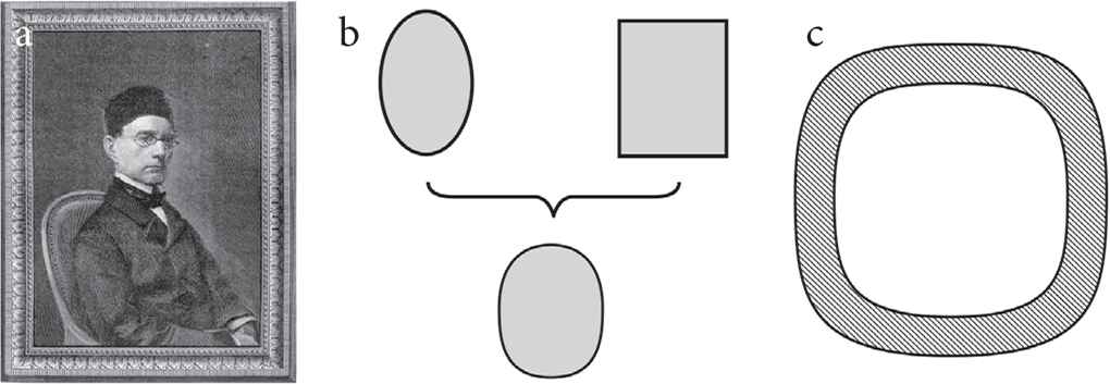
(a) Gabriel Lamé, (b) superellipses as optimal solutions, combining advantages of ellipse and rectangle, (c) cross section of square bamboo [4]

Addition is related to the arithmetic mean and multiplication to the geometric mean. Arithmetic and geometric means are found in every corner of mathematics and applied mathematics, in fundamental inequalities, such as the strict inequality ab<a+b2 (GM < AM) for any two positive integers. In the theory of surfaces, we have K ≤ H² where K and H are Gaussian and mean curvatures respectively, defined between the two principal curvatures κ₁, κ₂ in any point on the surface.

The Gaussian curvature is K = κ₁ · κ₂ (the square of GM) and the mean (or Germain) curvature is the arithmetic mean κ1+κ22 . Inequalities such as K ≤ H² are also known as natural curvature conditions. For exponential functions (and hence the logarithmic spiral) we have ρ = e^±nx for n = ±1. The product gives the geometric mean, which is constant along the curve ( e0=1 ). Half the sum is the arithmetic mean ex+e−x2 , and the definition of the catenary. Equality in the inequality GM ≤ AM is realised precisely in the lowest point of the catenary.

3.4. From Lamé Curves to Antonelli-metrics

The definition of classical means is also directly related to the measurement of distances. Lamé curves (Table 3) introduce anisotropy whereby lengths depend on the direction via Lamé curves, giving rise to the simplest Minkowski distances, with the classic Euclidean distance for n = 2 [7]:

with the taxicab metric for p = 1 and the max metric for p → ∞. Euclidean geometry is a special case for 1p+1q=1 in |x|^p + |y|^q = 1, or p = q = 2.

For distances there are two equally valid viewpoints, namely an internal and an external one. In superellipses in the 45° direction, the distance from the origin is either longer than in the 0° or 90° direction, when viewed with Euclidean glasses, or of the same length, when the supercircle is considered as a unit circle for the given Minkowski metric [4].

In ecology the Antonelli–Shimada metric [8] was introduced, which is the Finsler metric F = e^ϕ · L with L the p-th root metric of Minkowski (for integer p ≥ 3). This metric is used to study seismic wave propagation [9] in the framework of Finsler geometry. In |x˙a|p+|y˙b|p=1 , a and b express the anisotropy of the preferred orientation of aligned minerals along the earth’s surface and the Earth’s interior, respectively [9]. From this expression of the indicatrix (with a smooth wavefront) the fundamental function of the Lagrangian for crystal systems is changed into the generalized function for rocks (Eq. 13). Interestingly, the original motivation of Gabriel Lamé was the study of crystals [10].

The nature of wave propagation is explained by Huygens’ principle, where the envelope of the elementary wavefronts constitute a new wavefront, but in this anisotropic case the source point is not a point of minerals, but of a domain of rocks as a collection of minerals. For the seismic Finsler metric, the anisotropy of ray velocity is given by [9]:

This particular expression of Lamé curves in polar coordinates led to Gielis transformations [ Eq. (15)] originally introduced in Gielis [11]. It transforms a function f(θ), such as the above spirals or a constant function, such as R, the radius of a circle. This gives a stretchable radius or position vector. Equation (15) with m = 4, and p = n_1,2,3 is Eq. (14).

4.1. The Position Vector and the Equiangular Spirals

Two strong points of the polar coordinate system are (1) growth or development from one pole, and (2) the direct use of the position vector, one of the most important quantities in physics [12]. With the position vector curves can be defined kinematically. The catenary for example is the curve that the focus of a parabola traces, when this parabola is rolled without slipping on a straight line. Actually, the profile curves of all constant mean curvature surfaces (H = constant) can be obtained by rolling conic sections without slipping over a line, a fact proved by Delaunay [7].

In the plane, with constant vector length a circle is traced out, even if the rotation is continued for any number of cycles. In general, the length of the vector can change, monotonically, periodically or a combination of both. If the length increases with constant velocity, the result is the spiral of Archimedes. If the lengthening is by a constant acceleration, the result is the logarithmic or equiangular spirals [3] with the remarkable property that during growth the size changes, but not the form: Eadum mutata resurgo is the epitaph of Bernoulli.

The equiangular spiral can further be characterised as follows [13]:

As is well known, the equiangular spirals, i.e. the curves Γ in 𝔼2 for which the angle α = ∠ (X, X′) ∈ [0, π/2] between the tangent direction of the curve and the direction of its position vector is constant, are the logarithmic spirals ρ(θ) = k · e^aθ whereby a = cotg α and k is any real constant. And, conversely, these spirals geometrically define the natural logarithmic and exponential functions; …. the constant (π/4)-angled spiral with pole O and passing through the point E = (1,0) defines the natural exponential and logarithmic functions in a geometrical way: in particular this (π/4)-angled spiral defines the value of the natural exponential function by its distances ρ (θ) from the pole O for all angles θ∈𝕉.

Since the direction of the tangent fixes the direction of the normal, these conditions can also be expressed in terms of the normal direction.

Let T=X′||X′|| be the unit tangent vector field of a curve Γ in and let N = T^⊥ be the unit normal vector field, such that {T, N} is a positively oriented orthonormal frame field along Γ in 𝔼2 . Then, of course, for such a curve Γ to have constant angle α = ∠ (T, X) is equivalent to have constant angle α⊥=∠(N,X)=(π2 – α) and, so, the polar equation of the equiangular spirals with constant angle α or equivalently with constant angle α^⊥ can be rewritten as ρ (θ) = k · e^aθ with a = tg α^⊥.

The equiangular spirals can also be characterised is in terms of grad ρ [13]:

Since for a general curve ρ(θ) in 𝔼2 X′(θ) = ρ′(θ) · (cos θ, sin θ) + ρ (θ) · (−sin θ, cos θ), it follows that the arclength parameter s based at θ = 0 is given by s(θ)=∫0θ|| X′(θ)d(θ) ||  =∫0θ[ρ′2(θ)+ρ2(θ)]1/2dθ such that ds(θ)dθ=(ρ′2+ρ2)1/2(θ)

Hence dρ(θ)ds=[dρ(θ)dθ].[dθ(s)ds][ρ′(ρ′2+ρ2)1/2](θ), which shows that grad ρ = d ρ/ds = constant is a characterisation of the equiangular spirals in the Euclidean plane.

4.2. Constant Ratio Submanifolds

One of the quintessential examples of logarithmic spirals in nature is the shell of Nautilus. For the logarithmic spiral one finds that the force which makes a Nautilus shell grow can be decomposed into growth in length and width [12,13]. When considering a planar form as a result of growth, the constant ratio between the resolvents of the force of growth “in length and in width” (Figure 2), or between the radial component of growth and the component of growth in the direction perpendicular to the radial one, may be considered as one of the most natural laws of natural growth [12,13].

Figure 2

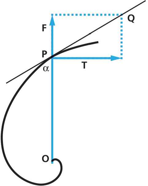
Components in logarithmic spiral [11]

This constant ratio aligns with contemporary differential geometry, which focuses strongly on submanifolds. A submanifold is a manifold immersed or embedded in another manifold, of the same or higher dimension. A square inscribed in a circle is one example (or any two Lamé curves); another one is a soap bubble floating in the air is a submanifold in a larger environment, called air. In general, such submanifolds have a constant ratio between the tangential x^T and normal component x^⊥ of position vector x. The submanifold is said to be of constant ratio if the ratio |xT||x⊥| is constant on M [12]. Constant ratio nD submanifolds Mⁿ in (n + m) dimensional Euclidean spaces are defined by one of the most natural conditions by which pure geometry may determine the shape of submanifold Mⁿ in 𝔼n+m [13]. The equiangular spiral is also a constant ratio submanifold in a plane. A circle is of constant ratio, because the angles between the tangent and the normal is 90° everywhere for every circle.

4.3. Spirals as Functions of Curvature and Arc Length

The curvature might also be interpreted as tension from within and tension induced by the surroundings. For this we need to look at spirals from the point of view of their curvature

as a function of arc length. The curvature of a circle is the inverse of the radius of that circle itself, and this measure of curvature, based on the circle, is used throughout science. For the circle, the curvature is constant along the arc, and dependent on the size of the circle with R=1κ . In the logarithmic spiral ρ = e^aθ, the parameter a defines the curvature of the spiral.

In general, plane curves whose curvature is a polynomial function of the arc length s are called polynomial spirals [14,15]. These spirals can be called Dillen-spirals, in honour of Franki Dillen (1963–2013). These polynomial spirals were a by-product of his classification of hypersurfaces Mⁿ of the (n + 1)-dimensional Euclidean space 𝕉n+1 with parallel higher order fundamental form, i.e. satisfying ∇^kh = 0 for some k, where h is the second fundamental form of Mⁿ [14].

For planar curves, if s goes to infinity the curvature function also goes to infinity. Since the curvature functions determines the curves up to an isometry (the fundamental theorem of Euclidean geometry), every spiral γ can be written as:

The curvature κγ(s)=P′κ(s) is then a polynomial of degree (k – 1) of s. The curves in Figure 3 correspond to κ = s; κ = s²; κ = s² – 2.19; κ = s² – 4; κ = s² +1; κ = 5s⁴ – 18s² + 5 respectively.

• •

  For k = 0, γ is a straight line.

• •

  For k = 1, γ is a circle.

• •

  For k = 2, γ is a Cornu spiral or chlotoid, a curve used by Cornu in 1874 in study on diffraction. Equation (17) has the Fresnel integral P_k (t) = t² as special case and is already found in Bernouilli’s Opera [14,15].

• •

  For k = 3, there are infinitely many non-similar curves. For κ = s² – D, with D∈𝕉 , the curve has two points of inflection for D > 0, one if D = 0 and none if D < 0.

Figure 3

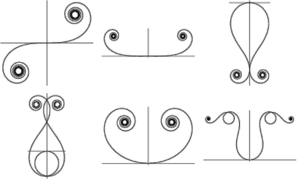
Dillen spirals

The measure of tension created in curves by their very shape as they evolve in terms of the polar angles is by X″, the angular curvature vector. ||X″|| = [(ρ″ – ρ)² – 4ρ′²)]^1/2 or rather its converse, gives a numerical measure of this angular tension [13]. This results from X″ (θ) = [ρ″ (θ) – ρ (θ)] · (cos θ, sin θ) + 2ρ′ (θ) · (−sin θ, cos θ).

4.4. Circle and Spirals: With or against the Flow

Curvature allows for the following characterisation of circle and logarithmic spiral as two curves with opposite tendency; which explains why these two curves are fundamental in the natural sciences. The second derivative describes the tension in the curve giving two possible opposites: Either position vector and tension vector are parallel X || X″, or they are orthogonal X ⊥ X″ ⇔ X · X″ = 0. The way of least resistance, growing in the direction parallel to the tension (circle) or the shape will resist the tension, growing in a direction perpendicular to the tension (a logarithmic spiral).

For a curve with parametrization X (θ) = (ρ (θ) cos θ, ρ (θ)sin θ), we have [16]:

X (θ) is the position vector and X″ (θ) the acceleration or tension vector, a measure for the tension in the curve. Two conditions are considered, which give the two most natural geometrical shapes in nature: the circle and the logarithmic spiral [13].

Condition 1: Position vector || to curvature vector: (X || X″) if the vector product equals zero. This condition translates as going with the flow, to align with the stress. For vectors in 𝕉3 with orthonormal base e⇀1,  e⇀2,  e⇀3

The solution is ρ′ = 0 or ρ = constant, which is a circle.

Condition 2: Position vector ⊥ to curvature vector: (X ⊥ X″) if the scalar product equals zero. This condition translates as going against the flow, to oppose the stress

For ρ (θ) ≠ 0: ρρ″ – ρ² = 0 or ρ″ = ρ. This is a family of solutions ρ (θ) = c₁e^θ + c₂e^−θ, with c_1,2 constants. For X (0) = (a, 0) and X′ (0) = (a, a), then c₁ + c₂ = a, c₁ – c₂ = a, so c₁ = a, c₂ = 0, which gives ρ (θ) = ae^θ.

Descartes searched for a curve for which in each point the position vector makes a fixed angle with the tangent vector. The parametrization X(θ) with ρ(θ) = ae^θ satisfies this condition, since X⋅X′|X||X′|=cosθ=c  (20) and X· X′ = a²e^2θ, |X| = ae^θ and |X′|=2aeθ , gives c=12  . Hence, the logarithmic spiral belongs to a family of curves for which X ⊥ X″ [13]. Curves growing from a pole such that their position vector permanently remains perpendicular to the direction of angular tension, defines the natural exponential function. For each angle θ, the radial distance ρ = d (0, X) determines the value of e^θ.

5.1. Anisotropic Curvature

Curvature is based on a point-wise approximation of a curve with a circle as in Sections 4.3 and 4.4. The radius of this circle is collinear with the normal to the curve. This goes back to Nicolas Oresme [17] and is the foundation of almost all of our scientific methods. It is a local operation and the only curve to which the circle is osculating globally (i.e. at each point on the curve a circle can be fitted of the same size) is the circle itself. This is based on the Pythagorean Theorem. Equation (15) however is a generalisation of the Pythagorean Theorem; indeed for all exponents m = 4, n_1,2,3 = 2, A = B = 1 the transformation equals 1 and describes a circle. Lamé curves are defined for m = 4, n_1,2,3 = n, or for m = 4, n₁ = p, n_2,3 = q [4,11,18].

Hence, the structure of Eq. (15) can be considered as Pythagorean-compact [4], and the resulting curves are unit circles. If measured against a classic circle, the radius stretches or shortens as a function of the angle, but if measured as its own, internal frame, the radius is constant (see Section 3.4). In the first case we have a variant of the classic Hooke’s Law F = kx, with force F and spring constant k (the external view point). In the second case however, x is a constant (radius of a unit circle) and the spring constant is variable k = f(x) defined by Eq. (15) (the internal view point). It is the point of view that matters, whether measurements are taken internally (unit circle) or from the outside, with a Euclidean ruler.

A most natural question to ask is if the internal measurements can be taken as a measure of curvature. This would mean that any shape defined by Eq. (15) for f (θ) constant with the classic unit circle for f (θ) = 1, can be approximated exactly by the shape itself [4]. In Figure 4a the classical Euclidean rotational symmetry is shown, whereby red and green starfish are rotated relative to each other and do not overlap. In Figure 4b a green starfish coincides with its totally osculating curve, the red starfish. In Figure 4c a chain of balls rolls around the curve. The shortest way for the chain to roll around the starfish curve is tracking the curve precisely along its perimeter, and the chain is then osculating, and everywhere or totally osculating when the chain becomes infinitely thin. In other words, rotating the red starfish of Figure 4a relative to the green one, it should follow the geometry of the space as in Figure 4b or the chain in Figure 4c.

Figure 4

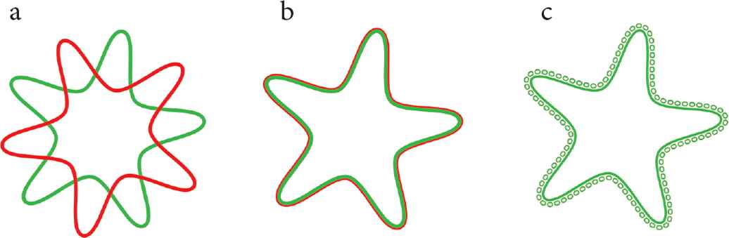
(a) Classical rotational symmetry of a starfish. (b) A starfish (green) with its totally osculating starfish (red), and (c) chain along a starfish [4]

The original shape and the curvature shape then become one and the same and are totally osculating. This may seem trivial but this same procedure has been at the core of science for many centuries with the classic Euclidean circle in Oresme’s tradition. Analogous to the classic definition of curvature κ=1R , using the inverse of the circle, we can define Lamé-curvature as:

or, curvature based on Gielis transformations for ϱ (υ; A, B, n₁, n₂, n₃) as:

As in the case of circles, the curvature is the inverse of the curve (unit circle) itself. Also, the transformations are Pythagorean compact and expressed in classical trigonometric functions. Moreover, each shape has its associated trigonometric functions and its dedicated half-length π_L or π_GT (which themselves can be expressed in terms of classical trigonometric functions). Eqs. (15), (21) and (22) can also be rewritten in terms of Chebyshev polynomials [4].

Curvature is the most important invariant of form and shape in science and mathematics. Using κ_GT not only allows for a precise (Pythagorean compact) description, but also the study of the evolution of curvatures. The Euclidean toolbox of transformations can be extended with Gielis tranformations.

5.2. Anisotropic Curvature in Natural Shapes

The main advantage of Eqs. (15), (21) and (22) in combination with Section 4.4, is that a shape can be split into one of two basic function (circle and spiral as basic shapes in nature) (Figure 5) and the specific Gielis transformation, which then defines the shape-specific curvature. The shape specific curvature can then directly inform us about the preferred anisotropic directions (as changes in the length of the position vector) if we consider anisotropy as deviation from Euclidean perfection (related to classical differential equations).

Figure 5

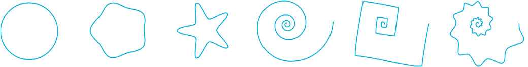
Transformations on basic shapes circle and spiral [7]

From an intrinsic or internal geometrical point of view the shapes are isotropic, with the same unit distance in all directions. Examples are given below for circles, Rhodonea curves and for the logarithmic spiral. All are expressed in polar coordinates following Loria’s definition in Section 1. A circle is a spiral with constant radius vector. It is also a spiral in the sense of curvature in function of arc length, since for k = 1 in Eq. (17), γ is a circle.

As first example, Figure 6 displays tree rings in oak, cedar and teak (Tectona grandis). Teak is notable for having square young stems and branches, which is reflected in tree rings in the early years (Figure 6a). In later years the annual tree rings are either getting more round, or in lower parts of the trunk, align with the anchoring system of the tree, e.g. oak (Figure 6b). Square sections can be found regularly in stems of Thuja occidentalis (Figure 6c). Annual tree rings reflect both the inherent anisotropy (building upon what is already there) and the influences of the year in which particular tree rings were built. Obviously, one can clearly separate the basic function circle and the anisotropy given by Eq. (15), with Lamé curvature κ_L defined by Eq. (21).

Figure 6

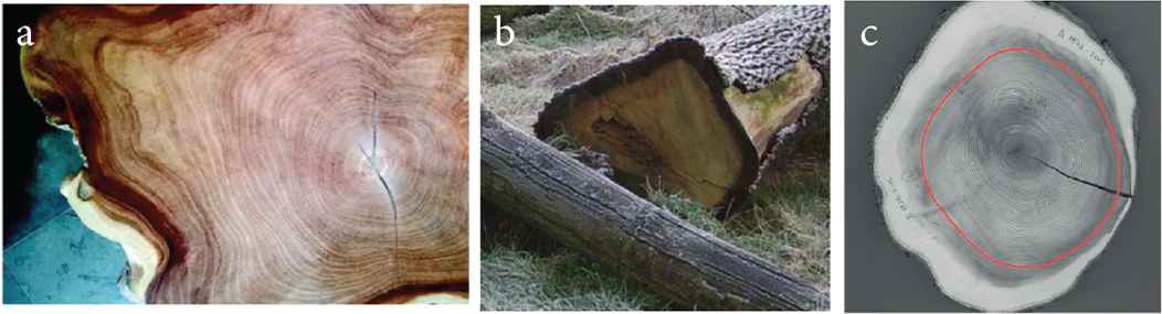
Tree rings in (a) teak, (b) oak, and (c) white cedar [4]

A second example are Rhodonea curves as sinusoidal spirals for ρ = cos nθ or ρ = sin nθ (Section 2.3). When these Rhodonea curves are subject to transformations by Eq. (15), flowers in Figure 7 lower row result. These can be considered as classical Euclidean rose or Rhodonea curves, forced or constrained to grow inside predefined polygons in Figure 7 upper row. In fact, such constraining can clearly be observed in the earliest stages of development in flowers [4].

Figure 7

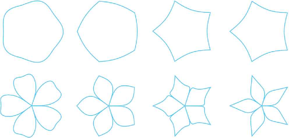
Flowers of Geranium, strawberry, Nicotiana and the corresponding Gielis polygons (upper row) [19]

These flowers are defined by Eq. (23) with parameter values in Table 4. They are directly related to the trigonometric functions associated with the m-polygons in the upper row of Figure 7, which are defined by Eq. (15).

Their expression using m/2 in itself is interesting, since this can be rewritten in terms of the recently defined pseudo-Chebyshev functions with T_(1/2) (x) = cos [(1/2) arccos x] and T_{(k + 1/2)} (x) = cos [(k + 1/2) arccos x] [3,20]. This means that not only the curvature of the polygons can be defined as κ_GT by Eq. (22), but also the curvature of the associated trigonometric functions.

As third example, shells of snails and Nautilus can be described as spirals with ρ (θ) = a · e^bθ. In most molluscs and ammonoids however, the length of the radius vector varies periodically (at least from the “Euclidean” point of view). For a = f (υ) defined by Eq. (15), we obtain Figure 8b, which is reflected in Trapezium horse conch (Figure 8a) and ammonoid like shells (Figure 8c). Once more, the Euclidean function can be separated from its curvature part κ_GT. In a wide variety of natural shapes, these transformations and curvatures describe both deviations from Euclidean perfection, and highlight the intrinsic anisotropy, which is imposed from the earliest stage of development.

Figure 8

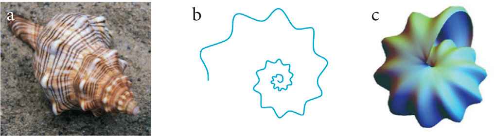
(a) Trapezium horse conch. (b and c) Logarithmic superspiral

Further examples are the Antonelli–Shimada metric and the seismic Finsler metric (14) with Lamé transformations κ_L on the basic functions: the m-th root metric of Minkowski in the first case, and n_1,2,3 = n, m = 4 in Eq. (15) in the second. The final example is the extension of the class of constant mean curvatures (CMC) (plane, cylinder, sphere, catenoid, undoloid and nodoid) to constant anisotropic mean curvatures (CAMC) surfaces [21]; they acquire shapes that are observed in e.g. snowflakes [4].