
Application of Logistic Regression Based on Maximum Likelihood Estimation to Predict Seismic Soil Liquefaction Occurrence
- DOI
- 10.2991/hcis.k.211207.001How to use a DOI?
- Keywords
- Probability of liquefaction; logistic regression; classification; maximum likelihood estimation; cone penetration test
- Abstract
Seismic soil liquefaction is one of the considerable challenges and disastrous sides of earthquakes that can generally happen in loose to medium saturated sandy soils. The in-situ cone penetration test (CPT) is a widely used index for evaluating the liquefaction characteristics of soils from different sites all over the world. To deal with the uncertainties of the models and the parameters on evaluating the liquefaction, a mathematical probabilistic model is applied via logistic regression, and the comprehensive CPT results are used to develop a model to predict the probability of liquefaction (PL). The new equation to assess the liquefaction occurrence is based on two important features from the expanded CPT dataset. The maximum likelihood estimation (MLE) method is applied to compute the model parameters by maximizing a likelihood function. In addition to that, the sampling bias is applied in the likelihood function via using the weighting factors. Five curve classifiers are plotted for different PL values and ranked using two evaluation metrics. Then, based on these metrics the optimal curve is selected and compared to a well-known deterministic model to validate it. This study also highlights the importance of the recall evaluation metric in the liquefaction occurrence evaluation. The experiment results indicate that the proposed method is outperform existing methods and presents the state-of-the-art in terms of probabilistic models.
- Copyright
- © 2021 The Authors. Publishing services by Atlantis Press International B.V.
- Open Access
- This is an open access article distributed under the CC BY-NC 4.0 license (http://creativecommons.org/licenses/by-nc/4.0/).
1. INTRODUCTION
The effects of soil liquefaction can be extremely catastrophic and may damage structures, infrastructures, and individuals’ lives. Soil liquefaction is a widespread phenomenon triggered by earthquakes that is mainly happen due to a combination of all three major factors: loose granular sediment, water-saturated sediment, and strong shaking. The Cone Penetration Test (CPT) is one of the most widely used indices for seismic liquefaction evaluation and it is one of the preferred simplified tests based on in situ tests due to the difficulty of performing soil dynamic laboratory tests and the expensive cost of sampling.
Researchers have applied probabilistic and deterministic models to predict and assess liquefaction occurrence. Considering the uncertainty of the model is what gives an advantage to probabilistic models over the deterministic ones. While deterministic models output is determined by the parameter values and the initial conditions, probabilistic models include some randomness, and the same parameter values and initial conditions may lead to different results. Generally, in deterministic model [1–5], in which a single boundary line as a classifier, is used to separate the liquefied from non-liquefied cases.
On the other hand, due to the uncertainties in the soil properties and sampling, it is more reasonable to represent models to predict liquefaction occurrence probabilistically rather than classical deterministic form. Several probabilistic models have been developed for liquefaction potential evaluation [6–10]. However, there is a shortage of models that are based on the expanded CPT dataset, which includes various sites with different features. Furthermore, the evaluation metrics do not include the recall metric, which is an important metric in such classification problems.
The logistic regression model is a widely used model for liquefaction potential assessment, which represents a bunch of triggering curves that classify the liquefaction and non-liquefaction cases. Logistic regression is a statistical model that is used for classification problems, the logistic regression had been used for the first time in the biological sciences of the early twentieth century [11,12]. Logistic regression is a supervised machine learning algorithm for classification problems yes/no, liquefied/non-liquefied, it is one of the most used classifiers in several fields such as Classification of Movement-Related Potentials [13], Predicting Mortality Risk of COVID-19 Patients [14], Determining landslide susceptibility [15,16]. Logistic regression utilizes a link function called sigmoid function (Equation 1) to limit the output value between zero and one and then based on a threshold the output is being mapped to one of the classes or categories.
To fit the logistic regression model coefficients, one of the most widely used approaches is applied, Maximum likelihood estimation (MLE) [17]. It is a statistical method of estimating a probability distribution coefficient by maximizing a likelihood function. The maximum likelihood does not have a closed-form solution which means it cannot be calculated in terms of a finite number of operations and functions, therefore, the problem is going to be solved using an optimization approach through the use of the gradient ascent algorithm.
Two types of uncertainties are distinguished, one of them depends on parameters and models, the other one depends on the uncertainty of sampling, soil properties, field laboratory tests,..., etc. To deal with the uncertainty of the parameters and the models, the probabilistic model is chosen instead of the deterministic one, and to deal with the uncertainties of the sampling and considering it, the weighting factor is applied to the likelihood function.
This paper uses the expanded case history in CPT dataset [5] and developed a new equation for the probability of liquefaction based on the logistic regression probabilistic model and two features; the equivalent clean sand normalized penetration resistance qc1N,cs and the cyclic stress ratio CSR7.5 as it is expressed in the Equation 10. The developed model has been evaluated using a very interesting metric which is recall, as the past studies have not considered the recall value in their assessments.
The recall metric gives the proportion of positive class identified correctly. Since predicting a liquefied data point as non-liquefied is considered to be more dangerous than predicting a non-liquefied data point as liquefied, and that is what the recall metric focuses on.
This study suggests a new equation to develop the seismic liquefaction triggering curve to classify the gravelly soil predictions. The new logistic regression equation is based on two features from the expanded CPT dataset that contains 251 data points from different earthquakes. The maximum likelihood estimation and the gradient ascent algorithm are used to estimate the value of the coefficients. Finally, the study highlights the importance of using logistic regression which is state-of-the-art in probabilistic models.
2. METHODOLOGY
To govern the uncertainty in liquefaction assessment, this study has employed a probabilistic model applying the logistic regression model to predict the occurrence of seismic soil liquefaction, probabilistic models using logistic regression have been performed by some researchers [18–20]. The maximum likelihood estimation is applied to fit the logistic regression coefficients by using the gradient ascent algorithm.
2.1. Logistic Regression
Logistic Regression (also known as logit) is a commonly employed classifier, used to assign the target value to a set of classes or categories. Two types of classification to be distinguished, the binary classification, in which the output can only take two classes, and the multiclass classification, in this type the output can take more than two classes. Using the sigmoid function (Equation 1), logistic regression converts the output which can then be mapped to two or more classes.
2.2. Maximum Likelihood Estimation
Maximum likelihood estimation (MLE) is a commonly employed method of estimating the parameters (also called weights or coefficients) of a probability distribution by maximizing the likelihood function (Equation 2). Bernoulli distribution is the distribution considered in this study which is an appropriate distribution for binary classification. The parameters that maximize the likelihood of the production of the data for m data points are considered as the logistic regression parameters.
In logistic regression, the likelihood function does not have a closed-form solution, therefore, the problem is solved using an optimization approach that is gradient ascent algorithm. Gradient ascent algorithm is the same as gradient descent, except maximizing instead of minimizing. It is much easier to maximize the log of the likelihood function instead of the likelihood function itself, by taking the log the product is converted to the sum. Since the logarithm is a monotonic function, this conversion would not affect the values of the parameters. Finally, to apply the gradient ascent algorithm, the partial derivative of the log-likelihood function is taken for each parameter.
The sampling bias effect should be considered in the sample data. Two major issues that trigger the sampling bias are; first one, the researchers and investigators implement in situ tests in liquefied sites more than non-liquefied tests; Secondly, the observed data and results can be collected and arranged based on the researchers’ knowledge and experience. Thus, the weighting factors for liquefied and non-liquefied cases WL and WNL (Equations 4 and 5) will be added to the likelihood function as shown in Equation 3, the weighted likelihood function has been used in several well-known studies [7,8,10].
The weighting factors estimation of WL and WNL (Equations 4 and 5,) was proposed by Ku et al. 2012 [8], in order to decrease the uncertainty in the sample.
NL is the total number of liquefied cases, and NNL is the total number of non-liquefied cases.
As it is mentioned before, it is easier to maximize the logarithm of likelihood by converting the product to the sum (Equation 6). Gradient ascent is an optimization algorithm that computes the weights (Algorithm 1), and here are the main steps of gradient ascent; 1. Initializing weights randomly. 2. Loop until convergence. 3. Computing the gradient
| Input: featuresL, features for the liquiefied cases, and featuresNL for non-liquiefied cases, number of iterations (numIterations) and learning step alpha (learningRate) | |
| Output: The coefficients(weights) of the sigmoid function θ0, θ1 and θ2 | |
| Method: Gradient ascent | |
| 1: | weights ← 0, 0, 0; |
| 2: | for (i ← 0; i < numIterations; i + +) do |
| 3: | scoresL ← np.dot(featuresL, weights); |
| 4: | scoresNL ← np.dot(featuresNL, weights); |
| 5: | predictionsL ← sigmoid(scoresL); |
| 6: | predictionsNL ← sigmoid(scoresNL); |
| 7: | ww ← np.dot((WL * featuresL.T), (1/(1 + np.exp(scoresL.T)))); |
| 8: | wx ← np.dot((WNL * −featuresNL.T), (1/(1 + np.exp(−scoresNL.T)))); |
| 9: | weights ← weights + learningRate * (ww + wx); |
| 10: | end for |
| 11: | return weights; |
Gradient ascent algorithm
2.3. Model Assessment Criteria
Two main evaluation metrics for classification problems were selected to perform the developed model and select the optimal one. The first one is the accuracy and the second one is the recall factor. Before explaining these two metrics and how they are calculated, it is important to first explain the confusion matrix which is a necessary part of computing accuracy and recall. The confusion matrix is a specific table layout to visualize the performance of our model’s prediction. As can be seen in Figure 1 each row of the matrix represents the instances in a predicted class, while each column represents the instances in an actual class.
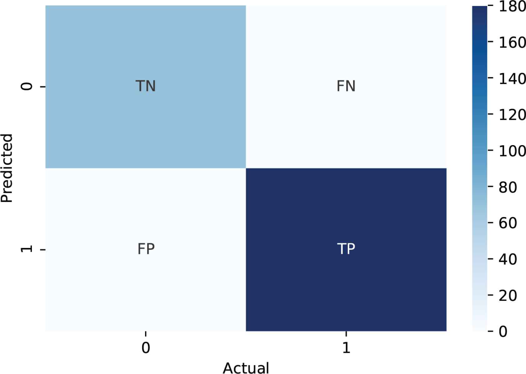
The confusion matrix layout.
0 is the negative class and 1 is the positive class. TP: or True Positives, means the number of cases where the actual class was 1 and also the predicted class was 1. TN: or True Negatives, means the number of cases where the actual class was 0 and also the predicted class was 0. FP: or False Positives, means the number of cases where the predicted class was positive 1 and the actual class was negative 0. FN: or False Negatives, means the number of cases where the predicted class was negative 0 and the actual class was positive 1.
The accuracy (Equation 8) is calculated then by dividing the total number of true predictions (TP + TN) by the total number of all the predictions (TP + TN + FP + FN).
Accuracy is not always the best metric to perform a model, especially for imbalanced classification problems, where a given class is representing the overwhelming majority of the data points in our dataset. So, for this reason, accuracy may not provide a better idea about our model performance. In this case, the metric we should focus on and maximize is known as recall (Equation 9).
False Negatives (FN) are the data points classified as non-liquefied that actually are liquefied. So, this is a major problem that should be considered while evaluating the model.
There are many other evaluation metrics for classification problems such as Precision, F1-Score, ROC, AUC,..., etc. To perform a comparison between the developed model and the deterministic model selected, only accuracy and recall metrics are chosen. For accuracy, it gives a general idea about how many data points were classified correctly, on the other hand, the recall metric is more accurate and gives a better intuition about our problem. Recall metric focuses more on the False Negatives, in our case the data points that are classified as non-liquefied but were liquified, so it is more important to maximize the Recall metric. In the selected deterministic model, the ROC and AUC metrics can not be calculated because it is a deterministic model and there is no threshold value.
3. PROPOSED MODEL AND COMPARISON WITH THE AVAILABLE MODEL
In this study, liquefaction occurrence prediction which is the output can only have two classes, class 0 for non-liquefied cases and class 1 for liquefied cases. To apply the logistic regression function on liquefaction assessment, the input of the sigmoid function z in the Equation 1 is set to θ T ⋅ X, θ T = (θ0 θ1 θ2) is the transpose matrix of the matrix
PL will produce the probability that the output is class 1 for liquefied. If PL 0.9 it gives a probability of 90% that the output is liquefied. the probability that the output is class 0 for non-liquefied is just the complement of the probability that it is class 1. For example, if the probability of class 1 is 90%, then the probability of class 0 is 10%.
In the liquefaction potential assessment considered in this study, the output variable yi can only have two possible values, 0 for no liquefied cases and 1 for liquefied cases. The probability of the target yi can be defined as follow:
3.1. Logistic Regression Model Based on Maximizing the Likelihood Function
The logistic regression model based on maximum likelihood estimation is proposed using the CPT index and considering the sampling bias by adding the weighting factors WL and WNL to the likelihood function. In Figure 2, five different curves were plotted for five PL levels (15%, 30%, 50%, 70%, and 90%). The way we plotted these curves is by applying the Equation 15 based on the same coefficients, the curves can be seen as thresholds for the logistic regression model. These curves are ranked based on the accuracy and recall metrics. The results are shown in Table 1. It can be concluded that the curve with PL = 50% seems to be the optimal one since it classifies the points ideally with the highest accuracy and recall values as it was expected. Despite the existence of curves (thresholds) with the highest recall value, but the commonly used and applied threshold in liquefaction occurrence evaluation is PL = 50%, if PL > 50% liquefaction occurs, else, no liquefaction is detected.
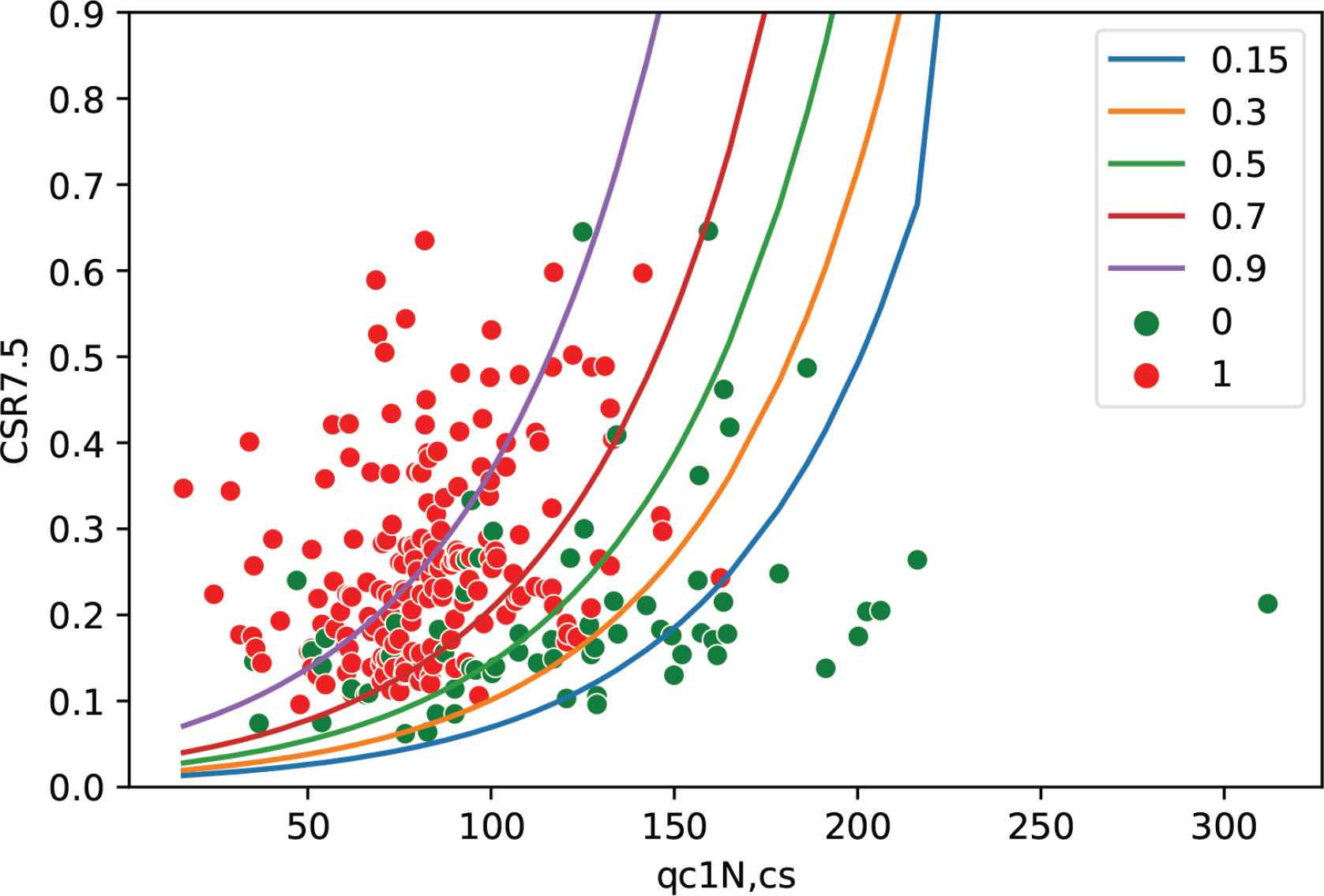
Different curve classifiers with different PL values.
| PL values | Accuracy | Recall |
|---|---|---|
| 15% | 79% | 100% |
| 30% | 82% | 99% |
| 50% | 84% | 94% |
| 70% | 80% | 83% |
| 90% | 56% | 42% |
Characteristics of the logistic regression models developed with different PL values
Before predicting liquefied or non-liquefied target based on the Logistic Regression model, three fitting coefficients should be computed based on maximum likelihood estimation (MLE), θ0 is the intercept or the bias, θ1 and θ2 are respectively the coefficients (weights) of the features qc1N,cs and ln(CSR7.5).
To estimate these coefficients or parameters, the dataset was derived from case history CPT documentation at different sites from different earthquakes all around the world. The dataset includes 180 liquefied and 71 non-liquefied cases, entirely 251 cases with several variables (features) including the main variables of CSR7.5 and qc1N,cs to develop triggering curve classification. The maximizing likelihood function is applied as an optimization algorithm for fitting curve parameters estimation. The model is then developed for PL equal to 15%, 30%, 50%, 70% and 90%, as can be seen in Figure 2.
Table 2 lists the coefficients, accuracy value, and recall value for the model developed for PL = 50%.
| This study’s model | Coefficients | Actual - predicted | ||||||
|---|---|---|---|---|---|---|---|---|
| ACC. | RECALL | θ0 | θ1 | θ2 | 0-0 | 0-1 | 1-1 | 1-0 |
| 0.84 | 0.94 | 9.192 | −0.046 | 2.362 | 43 | 28 | 170 | 10 |
Characteristics of the developed logistic regression model with PL = 50%
As mentioned before PL is the probability of predicting liquefied cases 1, consequently (1 – PL) is the probability of predicting non-liquefied cases 0. The weighting factors (WL and WNL) are included in the likelihood function (Equation 3) to calibrate the developed models. Finally, the optimal model is developed as below:
With WL = 0.6972 and WNL = 1.767, from Equations 4 and 5.
The receiver operating curve, also known as ROC, is one of the employed metrics to select the best threshold of the logistic regression model. It is a curve plotted by varying the threshold and computing the TPR and FPR (Equations 16 and 17) values for each threshold. Figure 3 shows the plotted ROC curve for the developed model, and the red point on the curve is the point with the optimal threshold which is 0.72, however, in the liquefaction occurrence classification, the threshold with the value of 0.5 seems to be optimal and the most commonly used one.
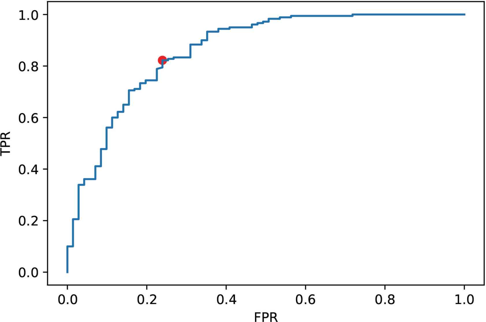
ROC curve for the developed model.
Due to the lack of data, the developed model is not verified using other data, the used expanded CPT dataset which contains 251 data points from different earthquakes is the only dataset used to build the model. There are some other datasets like SPT, DPT, Shear wave velocity dataset,..., etc, but the mentioned datasets do not include the same features and characteristics, that is why it is impossible to verify this study’s model using those datasets.
3.2. Comparison of the Logistic Regression Model Presented with the Available Model
The developed model in this study using probabilistic framework via logistic regression is compared to a well-known deterministic model proposed by Robertson and Wride [2] (Robertson’s model) for liquefaction potential evaluating, which is a CPT-based model with the same dataset and the same features to assess the liquefaction probability. The proposed model is then validated by comparing the triggering curves liquefaction assessment and the liquefaction occurrence predictions.
The reason behind choosing Robertson’s model to compare it with the developed model is that both models used the same features and the same dataset. Some of the logistic regression models mentioned in the first paragraph of the Methodology section, do not use the CPT dataset, and the others do not use the same features for studying liquefaction occurrence. Moreover, this study aims to prove the effectiveness of the probabilistic models over the deterministic models.
Robertson’s model as expressed in Equation 18, predicts the liquefaction target by comparing the Cyclic Resistance Ratio (CRR7.5) values with the Cyclic Stress Ratio (CSR7.5). The CRR7.5 > CSR7.5 predicts non-liquefied case and CRR7.5 < CSR7.5 shows liquefaction.
Robertson’s model assessment as listed in Table 3 provides 82% for accuracy and 88% for recall with 48 and 160 correct predictions of non-liquefied (True Negatives) and liquefied (True Positives) cases, respectively. In comparison with the model presented in this study for PL of 50%, the accuracy is 84% and recall is 94% with 43 and 170 accurate predictions of non-liquefied (True Negatives) and liquefied (True Positives) cases, respectively. The developed model for different PL values as shown in Figure 2, by increasing PL value, the curves move to the liquefied zone as it is expected. And for PL of less than 50% the graphs seem to be more conservative, which can be seen in Table 1. Figure 4 illustrates the comparison between the optimal model with PL = 50% and Robertson’s model. The two triggering curves liquefaction assessment are presented to classify the liquefied and non-liquefied cases. Predicting liquefied points as non-liquefied is a serious issue that the developed models should consider and have to minimize, and it is quite obvious that the model in this study has only 10 false-negative predictions meaning that the points were actually liquefied and the model classified them as non-liquefied, comparing to Robertson’s model which presents 20 false-negative predictions and that is a big number. This is where recall evaluation metrics come, it focuses more on the False Negatives (FN) value, and this metric should be maximized by minimizing the FN value.
| Robertson and Wride’s model | Actual - predicted | ||||
|---|---|---|---|---|---|
| ACC. | RECALL | 0-0 | 0-1 | 1-1 | 1-0 |
| 0.82 | 0.88 | 48 | 23 | 160 | 20 |
Characteristics of Robertson and Wride’s model
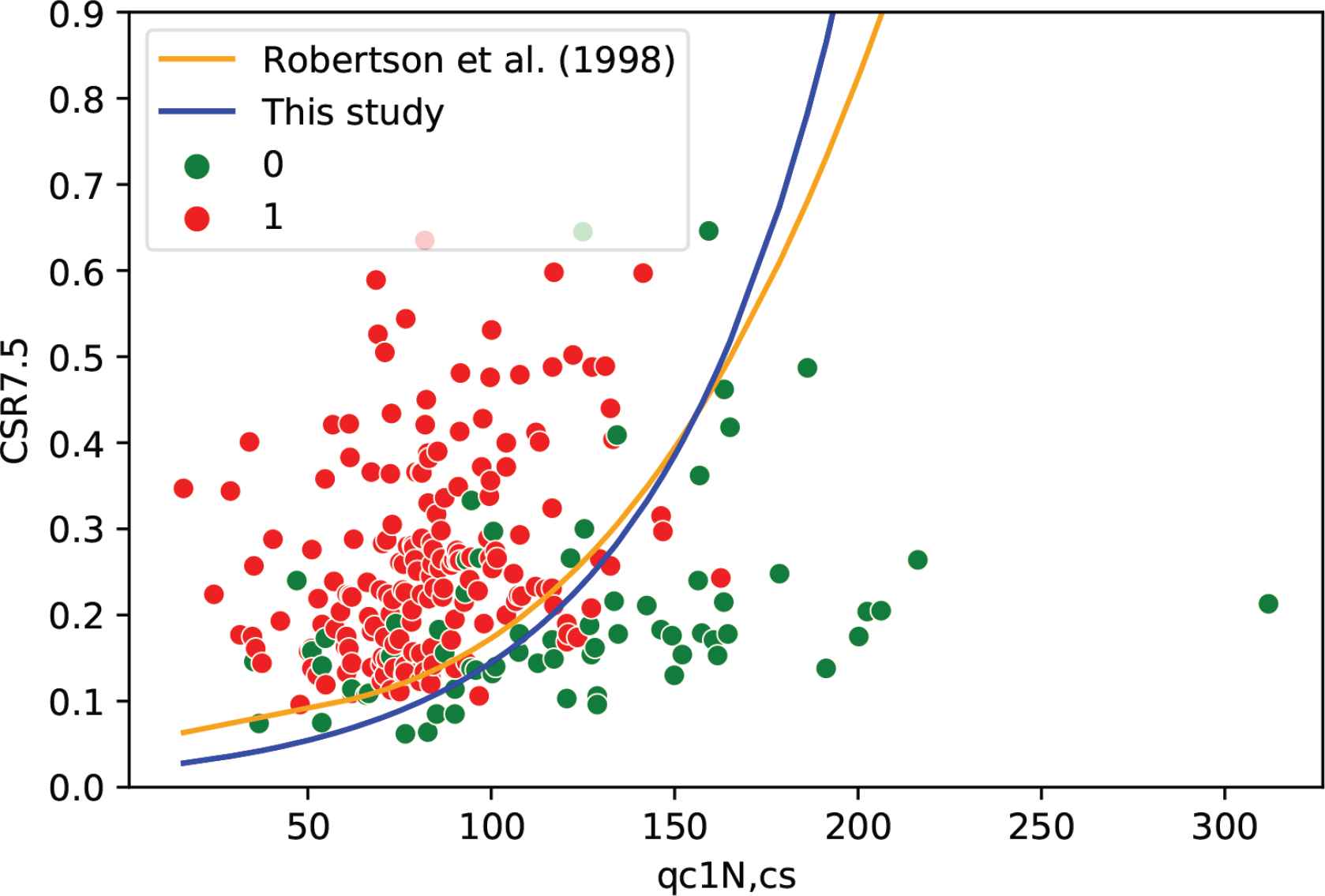
Performance of the proposed model and Robertson’s model.
This comparison shows that the probabilistic models are much better when it comes to liquefaction occurrence assessment. Probabilistic models can consider uncertainties and include some randomness, on the other hand, deterministic models do not include randomness and follow a definite equation of certainty. In Robertson’s model, the liquefaction occurrence is determined through the comparison between CRR7.5 and CSR7.5, if CRR7.5 > CSR7.5 no liquefaction is detected, else, liquefaction exists, and this is not always true, that is why it is highly recommended to develop and build probabilistic models over deterministic ones.
4. SUMMARY AND CONCLUSIONS
This study demonstrates the importance of developing probabilistic models rather than deterministic models to consider the uncertainties of the parameters and models. In this study, the probabilistic model is developed for liquefaction probability assessment based on the CPT dataset. The logistic regression model for classification and maximum likelihood estimation to determine the coefficients, the weighting factors are applied for the likelihood function to decrease the uncertainty in the sample and the model. Five curves for different PL values (15%, 30%, 50%, 70%, and 90%) are developed and ranked by the accuracy and recall evaluation metrics. Then, the optimal curve classifier has been selected and validated by comparing it with a well-known model’s prediction results. The experiment results indicate that the proposed method is outperform existing methods and presents the state-of-the-art in terms of probabilistic models. The main conclusions are summarized as follow:
- 1.
The logistic regression model which is a probabilistic model seems to be an optimal classifier and a better choice when it comes to liquefaction potential assessment.
- 2.
Among the five plotted PL curves developed, the curve with PL = 50% is the excellent classifier based on the accuracy and the recall evaluation metrics. The logistic model based on maximum likelihood estimation which is a probabilistic model is recommended for assessing liquefaction probability.
- 3.
The sampling bias is considered in the likelihood function to consider the uncertainty in the sampling. Ku et al. 2012 [8] approach to obtain weighting factors WL and WNL is effective for overcoming this shortage.
- 4.
The developed model in this study with PL = 50% provides an optimal classifier compared to Robertson’s model, with the highest accuracy and especially with the highest recall value which focuses more on the false negatives. In the liquefaction potential problem, false negatives are the datapoints predicted as not liquefied that actually were liquefied. Therefore, the presented model seems to be a safer risk assessment analysis of seismic liquefaction.
- 5.
The recall metric is a very important metric for assessing the liquefaction occurrence, it expresses the ability to extract all relevant instances from the dataset. Predicting a liquefied point as non-liquefied seems to be a very risky and catastrophic model. Therefore, the recall assessment criteria should be maximized and that was the case of the developed model which shows a higher capability and economic model for risk assessment and predicting liquefaction occurrence. In the five developed curves, the recall value decreases by increasing the PL value, and that was expected because as the PL value increases the total number of false negatives increases too, consequently, the recall decreases.
CONFLICTS OF INTEREST
The authors declare they have no conflicts of interest.
AUTHORS’ CONTRIBUTION
Idriss Jairi contributed in writing, methodology, data preprocessing, software. Yu Fang contributed in conceptualization, writing – reviewing, supervising. Nima Pirhadi contributed in editing, reviewing, validating.
ACKNOWLEDGMENTS
This work is supported by the National Natural Science Foundation of China (No. 62006200); the Project of SiChuan Youth Science and Technology Innovation Team (No. 2019JDTD0017); the first-class undergraduate course construction project of Southwest Petroleum University (X2021YLKC035) and Southwest Petroleum University Postgraduate English Course Construction Project (No. 2020QY04).
ETHICAL APPROVAL
This article does not contain any studies with animals performed by any of the authors.
REFERENCES
Cite this article
TY  - JOUR
AU  - Idriss Jairi
AU  - Yu Fang
AU  - Nima Pirhadi
PY  - 2021
DA  - 2021/12/11
TI  - Application of Logistic Regression Based on Maximum Likelihood Estimation to Predict Seismic Soil Liquefaction Occurrence
JO  - Human-Centric Intelligent Systems
SP  - 98
EP  - 104
VL  - 1
IS  - 3-4
SN  - 2667-1336
UR  - https://doi.org/10.2991/hcis.k.211207.001
DO  - 10.2991/hcis.k.211207.001
ID  - Jairi2021
ER  -