
A New Rewarding Mechanism for Branching Heuristic in SAT Solvers
- DOI
- 10.2991/ijcis.2019.125905649How to use a DOI?
- Keywords
- Satisfiability problem; Conflict-driven clause learning; Branching heuristic; Literal block distance
- Abstract
Decision heuristic strategy can be viewed as one of the most central features of state-of-the-art conflict-driven clause-learning SAT solvers. Variable state independent decaying sum (VSIDS) still is the dominant branching heuristics because of its low cost. VSIDS consists of a rewarding mechanism for variables participating in the conflict. This paper proposes a new rewarding mechanism for branching strategy, rewarding variables differently depended on information provided by the conflict analysis process, that is to say, the literal block distance value of the learnt clause and the size of the backtrack level decided by the learnt clause. We implement it as part of the Glucose 3.0 solver and MapleCOMSPS solver. Compared with Glucose 3.0, the number of solved instances of the improved Glucose_LBD + BTL is enhanced by 6.0%; compared with MapleCOMSPS, the number of solved instances of MapleCOMSPS_LBD + BTL is added by 3.4%. These empirical results further shed light on the proposed heuristic having the advantage of solving Application benchmark from the SAT Competitions 2015–2017.
- Copyright
- © 2019 The Authors. Published by Atlantis Press SARL.
- Open Access
- This is an open access article distributed under the CC BY-NC 4.0 license (http://creativecommons.org/licenses/by-nc/4.0/).
1. INTRODUCTION
The Boolean satisfiability (SAT) problem decides whether exists an assignment that makes the given formula (which expressed in Conjunctive Normal Form (CNF)) true or not. A formula F is a conjunction of clauses C, that is, F = ∧C, and each clause C is a disjunction of literals l, e.g., C = ∨l. A literal l refers to either a positive variable x or a negative variable x. A truth value for a Boolean variable x is: x → {0,1}. It is best known for its theoretical importance which has proved to be NP-Complete [1]. Many hard combinatorial problems arise in formal verification [2], artificial intelligence [3], data mining [4], machine learning [5], mathematics [6], and so on, can be encoded as SAT formula. Indeed, from the theoretical and practical perspective, a vast array of advances in SAT research over the past twenty years have contributed to making SAT technology an indispensable tool in a variety of domains.
SAT solvers can generally be divided into two architectures: complete and incomplete solvers. Although incomplete algorithm especially salient for targeting satisfiable random SAT formula, it is unable to prove unsatisfiability. Indeed, a large variety of formula, generating from real-world utilities, needed to be proved unsatisfiability. Consequently, complete SAT solvers are a requirement. State-of-the-art complete SAT solvers are predominantly based on conflict-driven clause learning (CDCL) [7] algorithm, which extends the Davis–Putnam–Logemann–Loveland (DPLL) algorithm [8] by adding effective search techniques, including fast Boolean constraint propagate (BCP), variable state independent decaying sum (VSIDS) branching heuristics [9], clause learning (result of the resolution refutation), restarts [10], and a lazy data structure [11]. These techniques spawn tremendous gains in the efficiency of SAT solvers.
One of the most surprising aspects of the relatively recent practical progress of CDCL solvers is decision selection heuristics, which choose a decision variable to branch on. Varying decision variable extremely influences the efficiency of the solver. Different branching heuristics for the same problem may result in completely different computational results [12, 13], because of the binary search tree determined by different decision variables varies greatly. It is well known that a “good” decision heuristic is virtual and the problem of choosing the optimal variable in DPLL algorithm had been proven to be NP-hard as well as coNP-hard [14]. Researchers proposed multiple varying decision heuristics after all these years, for instance, Bohm’s heuristic [15], maximum occurrences on minimum sized clauses (MOM) [16], and Jeroslow–Wang [17]. Marques-Silva had done comparative experimental evaluations about these above heuristic strategies in the solver GRASP, and found that none was a clear winner. Subsequently, literal count heuristics were derived [12]. In particular, dynamic largest combined sum (DLCS), dynamic largest individual sum (DLIS), and rand dynamic largest individual sum (RDLIS) are all of literal count heuristics, that is, choosing a variable or literal with the highest frequency that occurring among the yet unsatisfied clauses. VSIDS, an even more aggressive dynamic scoring scheme, was proposed in Ref. [9]. Up to now, VSIDS and its variants continue to be the dominant branching heuristics among competitive SAT solvers such as Minisat [18], Glucose [19], Lingeling [20], and CryptoMiniSat [21], because of its robustness, even though VSIDS initially was proposed sixteen years ago. Lots of researches employ further variations on VSIDS, such as exponential VSIDS (EVSIDS) [22], Rsat [23], variable move-to-front (VMTF) [24], and average conflict-index decision score (ACIDS) [25]. The empirical evaluation of Ref. [25] shows that EVSIDS, VMTF, and ACIDS empirically perform equally well.
Such a family of heuristics always kept a score for each variable and rewarded a constant value which responsible for conflicts analysis. Ref. [26] proposed a method of rewarding variables with different scores depending on the character of the conflict whenever a conflict occurs. Ref. [27] developed a different rewarding mechanism based on the information provided by search algorithm, namely the size of learned clauses and the size of backjumps in the search tree. Ref. [28] proposed a clause-based heuristic, chosen the next decision variable from the top-most unsatisfied clause. The solver MapleCOMPSP [29] won a gold medal for Application Main Track benchmarks in SAT Competition 2016, proposed a new branching heuristic called learning rate branching (LRB), which selected variable with a high learning rate, that is, maximizing generate a quantity of learnt clauses. In SAT Competition 2017, the solver Maple_LCM_Dist [30], got the first prize for Application Main Track benchmarks, presented a heuristic based on distance, that is rewarding a variable which had the longest distance in the implication graph at the beginning of searching. Ref. [31] proposed to reward more variables that yield are involved in learnt clauses with small literal block distance (LBD). Based on Ref. [31], in this paper, we propose a new heuristic strategy, rewarding variables differently on the basis of the characteristics of the problem. Namely, the proposed rewarding mechanism is to reward variables that are involved in creating small LBD value and contributed to backtrack to the large level during the conflict analysis process. The experimental results indicate that the proposed rewarding mechanism obtains significant gains for solving Application benchmark from the SAT Competitions 2015–2017.
The remaining part of this paper is organized as follows: Section 2 introduces the framework of CDCL algorithm and provides an example to illustrate conflict analysis and clause learning. In Section 3, we describe our proposed decision heuristic in detail. Section 4 presents the experimental results, showing that the performance of our solver Glucose_LBD + BTL is improved dramatically after adopting the proposed strategy, our solver MapleCOMSPS_LBD + BTL is competitive with respect to the top solver MapleCOMSPS. Finally, we draw conclusions in Section 5.
2. CDCL ALGORITHM
The CDCL algorithm is predominantly an extension of the original DPLL algorithm.
2.1. CDCL Algorithm
Algorithm 1 lists the typical form of the CDCL algorithm.
Algorithm 1 Typical CDCL Algorithm
| Input: | Formula F in CNF |
| Output: | SAT or UNSAT |
| 1: | clauses ←clausesOf(F) |
| 2: | v ← ∅ // variable assignment set |
| 3: | level←0 // decision level, also known as restart level |
| 4: | if(UnitPropagation (clauses, v) == CONFLICT) |
| 5: | then return UNSAT |
| 7: | else |
| 8: | while True do |
| 9: | var = PickDecisionVar(clauses, v) |
| 10: | if no var is selected // all variables are instantiated |
| 11: | then return SAT |
| 12: | else |
| 13: | level←level + 1 |
| 14: | v←v ⋃ {var} |
| 15: | while(UnitPropagation(clauses, v) == CONFLICT) do |
| 16: | learned = AnalyzeConflict(clauses, v) |
| 17: | clauses←clauses ⋃ {learned} |
| 18: | dlevel = Computedlevel(clauses, v) |
| 19: | if(dlevel == 0) //conflict at decision level 0 |
| 20: | then return UNSAT |
| 21: | else |
| 22: | BackTrack(clauses, v, dlevel) |
| 23: | level←dlevel |
| 24: | end while |
| 25: | end while |
There are two significant functions: the PickDecisionVar() function and AnalyzeConflict() function. The procedure PickDecisionVar(), an aspect of decision heuristic strategy, chooses an unassigned variable to assign by applying either a static or a dynamic decision heuristic. Modern competitive CDCL SAT solvers still adopt VSIDS and its variants as the decision strategy. VSIDS associates a floating point number score s(l) for each literal l. Initially, the score s(l) is equivalent to the literal’s activity, the frequency of a literal occurrence in all clauses. As the stated above, whenever a learnt clause C is added to the clause database in order to block the same conflicts, VSIDS dynamically increments the score s(l) of variable by one, which is contained in learnt clause C. VSIDS will choose the unassigned literal with the maximum combined score to branch during the search process. Ties are broken randomly by default. Moreover, all score periodically is decreased by multiplying a float point constant between 0 and 1, also called the decay. In this way, these literals that do not participate in conflicts for a long time are penalized. Clearly, the scores are not dependent on the variable assignments, called the state independent, which does not require to traverse the clause database at decision variable selection, and the score only needed to update when conflict occurs, so it is cheap to maintain. Thus, VSIDS had turned out to be quite adequate for solving a problem, being characterized by having a negligible computational overhead. The state-of-the-art VSIDS sorts variables in an array, and the array is sorted w.r.t. decreasing score when updates score periodically, further, every 256th conflict.
The AnalyzeConflict() function, which is part of the most important characters, generates a learnt clause and adds it to the set of clauses, and also contains ComputeDLevel() and BackTrack() procedure. The function ComputeDLevel() computes the backtrack level dlevel that is needed for BackTrack(). If dlevel is equal to 0, then it means that there exists a variable, which must be assigned true and false in the meantime. As a consequence, formula F must be unsatisfiable. If not, we perform the backtracking by removing assignments between the current level and the backtrack level dlevel, and update the current level indicator.
2.2. Conflict Analysis and Clause Learning
Consider the example formula F.
F: C1 = −x8 ∨ x2
C2 = −x1 ∨ x4
C3 = −x1 ∨ x7
C4 = x5 ∨ −x9
C5 = −x1 ∨ x6 ∨ x8
C6 = −x3 ∨ −x4 ∨ −x6 ∨ −x7
C7 = −x3 ∨ x10 ∨ −x11
C8 = −x2 ∨ −x5 ∨ −x10
C9 = x9 ∨ −x10 ∨ −x12
Figure 1 illustrates an implication graph, which is a directed acyclic graph. Each vertex represents a literal associated with its current assignment and its decision level. If the vertex of literal has no incoming edges, it is the decision literal. A directed edge from vertex xi to vertex xj reveals that the assignment of literal xi implies the assignment of literal xj, which is induced by BCP. The decision level of an assigned variable is added by one from level 1 whenever each decision literal is assigned. For example, x1(5) is a decision literal, and it is assigned true, and its relevant decision level is 5. Since x1 implies x4, the decision level of x4 also is 5. “□” presents the corresponding falsified clause “
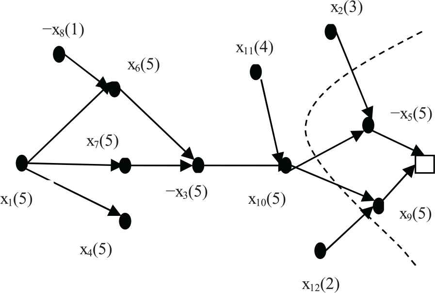
Logical implication graph of F.
3. A NEW REWARDING MECHANISM
As mentioned earlier, modern VSIDS method favours variables that participate in either a learnt clause (particularly recent learnt clauses) or the conflict side of the implication graph. Back to the example in Section 2.2, the learnt clause is
Figure 2 shows the generation process of learnt clause utilizing resolution rule. We can see from Figure 2 that those variables {x2, x10, x12, x9, x5} are responsible for conflict analysis, and these variables are more constrained than others. Certain branching heuristic strategies, extended the VSIDS strategy, increased the activity of those corresponding variable by 1 only.
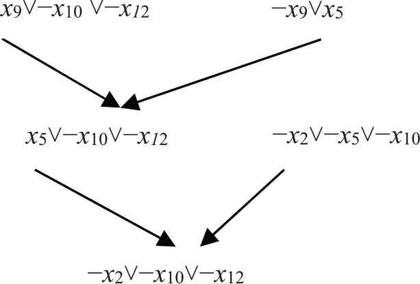
Generation process of learnt clause.
The effect of learnt clause is mainly reflected in the following two aspects: on the one hand, the learnt clause succinctly expresses the cause of conflict. The more the variable is associated with constructing the conflict, the larger its activity. Those heuristics always choose variable with the highest activity as the branching variable, so, it is easy to find those conflicts which had been happened. Such learnt clause is then used to prune the search space; on the other hand, the learnt clause decides how far to backtrack by analyzing the decision level of variables contained in the learnt clause. Therefore, based on the function of learnt clauses, we define a new rewarding mechanism of variable score value. An equation as follows:
3.1. Set Rlbd Parameter
Because intractable problems generate numerous conflicts in the solution process, thereby lots of learnt clauses are produced. Meanwhile, learnt clauses are considered as resolution-based producers of clauses and can prune search space that remained to be searched, learnt clause is the primary driving force for solving the difficult problem. In general, different learnt clause effect on the solution of an instance largely. It is an obviously significant challenge to identify good learnt clauses. More recently, in Ref. [19], Audemard et al. proposed an accurate measure, LBD, estimating the quality of a learnt clause. The LBD is defined as follows: “Given a clause C, and a partition of its literals into n subsets according to the current assignment, s.t. literals are partitioned w.r.t their level. The LBD of C is exactly n.” Based on experimental results [19], clauses with small LBD value are considered more useful than those with high LBD value. The LBD value of a given clause is lower, this clause needs the number of decisions is fewer in unit propagation. Intuitively, it is easy to understand the importance of glue clauses, that is, clauses with LBD value of 2, because of the 1-UIP, the glue clauses just contain one variable of the recent decision level, accordingly, the variable will be glued with the block of literals propagated above, no matter the size of the clause. This makes sense in light of the fact that the lower the LBD value of learnt clause, the more it is utilized in the subsequent solving process. Here, if a learnt clause causes conflict or propagation, we consider it is utilizable. In order to validate the assumption, experiments are tested on the following SAT instance: vmpc_29.cnf, which originated from 2015 SAT benchmark.
Figure 3 presents the total number of times learnt clause with a given LBD value is utilized in the solution process. The x-axis denotes a given LBD value while the y-axis denotes the total number of times. In this experiment, a counter is jointed with each LBD value x, and the counter is increased whenever a learnt clause of LBD equal to x is utilized. As we can observe from Figure 3, a learnt clause with lower LBD value are utilized more frequently during solving process than those with higher LBD value. Since variables involved in a learnt clause of smaller LBD are significant than those involved in learnt clause of higher LBD, therefore, we define the Rlbd parameter of a learnt clause c: Rlbd = 1/LBD (c).
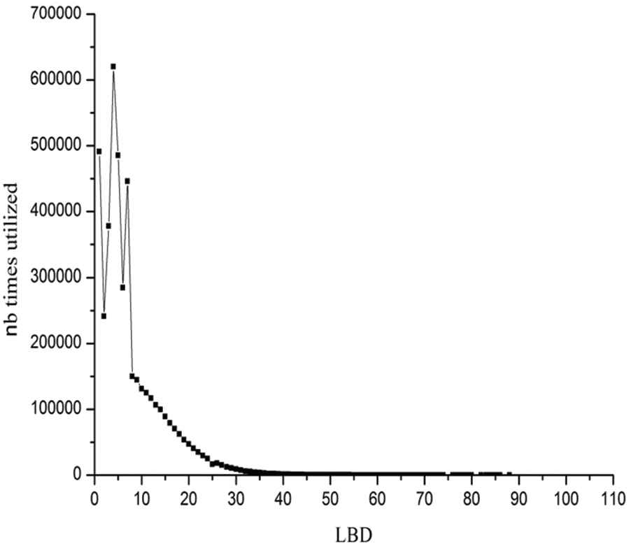
Number of times learnt clauses with a given literal block distance (LBD) value are utilized.
3.2. Set Rbtl Parameter
Let us consider again the learnt clause Number of times learnt clauses with a given BTL value are utilized.
3.3. LBD and BTL
To further illustrate the relationship between LBD value and BTL value, we continue to test on the vmpc_29.cnf instance. In the interest of distinctly observe the varying of LBD value and BTL value in solving process, Figure 5 presents the LBD values and BTL values corresponding to the only first 1000 learnt clauses.
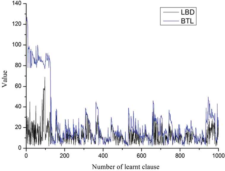
Relationship between literal block distance (LBD) and BTL.
In Figure 5, the x-axis means each learnt clause and the y-axis presents the LBD value and BTL value of learnt clause. The black (blue) line represents the LBD (BTL) value, respectively
It can be seen from Figure 5 that the change trend of LBD and BTL is basically consistent, that is, if the LBD value of learnt clause is large, the BTL value is also large, and vice versa. This indicates that when the score value of variable can be updated according to Equation (2), it is probably to select those variables with strong constraint ability to the solution space in the branching strategy.
4. EXPERIMENTAL RESULTS
We implemented the new rewarding mechanism described in Section 3 based on Glucose 3.0 [33] solver, that was used to determine the difficulty level of each benchmark for the SAT Competition in recent years. The resulting solvers are named Glucose_LBD, Glucose_BTL and Glucose_LBD + BTL, respectively. Glucose_LBD rewards variables with 1/LBD value only, similarly, Glucose_BTL rewards variables with 1/BTL value only, and Glucose_LBD + BTL implements the rewarding approach depending to Equation (2). The experiment was implemented on a 64-bit machine with 8Gb of memory and Intel Core i3-3240 CPU 3.40 GHz processor. The test instances originated from the application track (obtained from a diverse set of applications) of the 2015, 2016 and 2017 SAT Competitions [34–36]. For each instance, the solver is allocated 3600 seconds of CPU time.
Table 1 compares the number of solved instances by the four solvers Glucose 3.0, Glucose_LBD, Glucose_BTL, and Glucose_LBD + BTL. The numbers shown in the table are intended to be indicative. Our rewarding method consistently improves the performance of all the solvers configured with the new rewarding method. The Glucose_LBD (Glucose_BTL) solved 19(14) instances more than Glucose 3.0, respectively. Furthermore, the performance of solver Glucose_LBD is better than Glucose_BTL. In particular, Glucose_LBD + BTL is the best solver, and it solved 30 instances more than Glucose 3.0, the total number of solved instances by Glucose_LBD + BTL is increasing by 6.0% compared with Glucose 3.0 solver. In order to better demonstrate the performance of the proposed strategy, we quote two of the leading SAT solver developers Professors Audemard and Simon [19]: “We must also say, as a preliminary, that improving SAT solvers is often a cruel world. To give an idea, improving a solver by solving at least ten more instances (on a fixed set of benchmarks of a competition) is generally showing a critical new feature. In general, the winner of a competition is decided based on a couple of additional solved benchmarks.” From Table 1, it can be seen clearly that our proposed strategy has better performance for instances.
| Benchmarks | Status | Glucose 3.0 | Glucose_LBD | Glucose_BTL | Glucose_LBD + BTL |
|---|---|---|---|---|---|
| Sat 2015 (300) | sat | 137 | 145 | 144 | 150 |
| unsat | 93 | 97 | 94 | 98 | |
| sum | 230 | 242 | 238 | 248 | |
| SAT 2016 (300) | sat | 56 | 58 | 57 | 62 |
| unsat | 76 | 77 | 78 | 76 | |
| sum | 132 | 135 | 135 | 138 | |
| SAT 2017 (350) | sat | 72 | 74 | 74 | 82 |
| unsat | 69 | 71 | 70 | 65 | |
| sum | 141 | 145 | 144 | 147 | |
| Total (950) | sat | 265 | 277 | 275 | 294 |
| unsat | 238 | 245 | 242 | 239 | |
| sum | 503 | 522 | 517 | 533 |
Comparison of Glucose 3.0, Glucose_LBD, Glucose_BTL, and Glucose_LBD + BTL on Instances.
Figure 6 shows the cactus plot comparing the performance comparison of these four solvers. The x-axis denotes the numbers of solved instances while the y-axis denotes the time required to solve them. The line is farther in the right, it means that more instances are solved by the corresponding solver. Meanwhile, lower the line, faster the corresponding solver works. As can be seen from the cactus plot in Figure 6, the Glucose_LBD + BTL solver has the best solving performance.
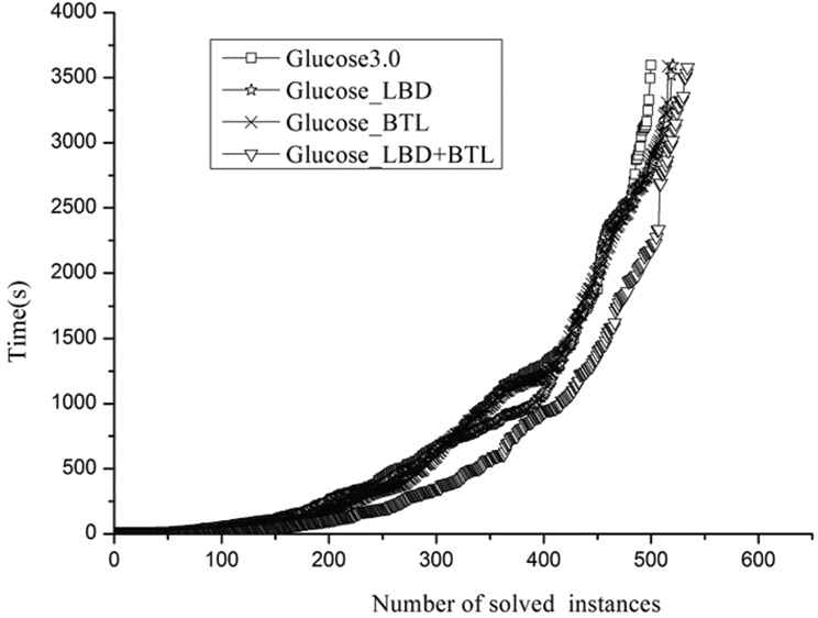
Cactus plots of Glucose 3.0, Glucose_LBD, Glucose_BTL, and Glucose_LBD + BTL on instances.
Figure 7–9 presents a log–log sample of scatter plots comparing Glucose 3.0 runtime and Gluocose_LBD_BTL running on 3 benchmark families derived from industrial application.
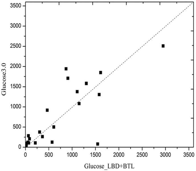
Scatter plots comparing Glucose 3.0 runtime and Gluocose_LBD_BTL running on cryptography benchmark families.
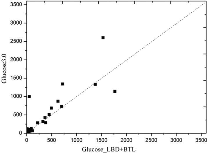
Scatter plots comparing Glucose 3.0 runtime and Gluocose_LBD_BTL running on SATPlanning benchmark families.
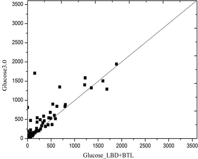
Scatter plots comparing Glucose 3.0 runtime and Gluocose_LBD_BTL running on Velev benchmark families.
A family consists of instances with similar names. Cryptography benchmark is generated as part of an attack on the Bivium stream cipher [37]. We use 46 instances. SATPlanning benchmark is generated from transport application provided by Rintanen [38], we use 44 instances. Velev benchmark consists of an ensemble of hardware formal verification problems distributed by Miroslav Velev [39]. We use 195 instances. Each dot represents an instance, x-axis (resp. y-axis) corresponds to the time needed by Gluocose_LBD_BTL (resp. Glucose 3.0) to solve an instance. The dots below the diagonal imply that instances were solved faster with Gluocose_LBD_BTL solver. As shown in Figure 7–9, Gluocose_LBD_BTL is faster than Glucose 3.0 because of most dots below the diagonal.
To better illustrate the advantages of the proposed method, we further compare with MapleCOMSPS solver, which took the first place in the Main-track group of SAT 2016 competition. Table 2 presents the number of solved instances by MapleCOMSPS and MapleCOMSPS_LBD + BTL solver. Note that, MapleCOMSPS_LBD + BTL is the modified version solver configured with our proposed method. The modified MapleCOMSPS_LBD + BTL solver can be able to solve up to 19 additional instances compared with MapleCOMSPS, and the total number of solved instances by MapleCOMSPS_LBD + BTL is increasing by 3.4%.
| Benchmarks | Status | MapleCOMSPS | MapleCOMSPS_LBD + BTL |
|---|---|---|---|
| Sat 2015 (300) | sat | 154 | 157 |
| unsat | 102 | 102 | |
| sum | 256 | 259 | |
| SAT 2016 (300) | sat | 65 | 78 |
| unsat | 78 | 70 | |
| sum | 143 | 148 | |
| SAT 2017 (350) | sat | 90 | 91 |
| unsat | 68 | 78 | |
| sum | 158 | 169 | |
| Total (950) | sat | 309 | 326 |
| unsat | 248 | 250 | |
| sum | 557 | 576 |
Comparison of MapleCOMSPS and MapleCOMSPS_LBD + BTL on Instances.
Figure 10 shows the cactus plot comparing the performance of MapleCOMSPS_LBD + BTL against the MapleCOMSPS solver. As can be seen from Figure 10, the cactus of MapleCOMSPS_LBD + BTL is right and below the curve of MapleCOMSPS. It implies that MapleCOMSPS_LBD + BTL outperforms MapleCOMSPS. These results provide evidence of the effectiveness of our proposed approach.
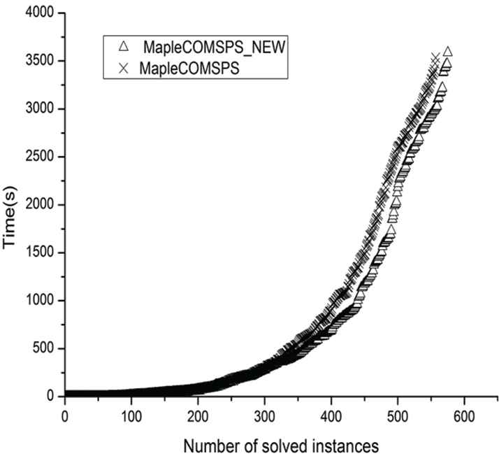
Performance of MapleCOMSPS_LBD + BTL versus MapleCOMSPS over instances.
5. CONCLUSION
In this paper, we propose a new heuristic strategy, rewarding variables with varying values, based on the LBD value of each learnt clause, and the backtrack level. The approach is simple and can be implemented in a CDCL SAT solver. We implemented the proposed strategy on Glucose 3.0 and MapleCOMSPS, respectively. The experimental results demonstrate that our modified solvers have better performance than those Glucose 3.0 and MapleCOMSPS solvers for solving Application benchmark from the SAT Competitions 2015–2017.
ACKNOWLEDGMENTS
This work is supported by the National Natural Science Foundation of China (Grant No. 61673320), and by the Fundamental Research Funds for the Central Universities (Grant No. 2682018ZT10).
REFERENCES
Cite this article
TY  - JOUR
AU  - Wenjing Chang
AU  - Yang Xu
AU  - Shuwei Chen
PY  - 2019
DA  - 2019/01/28
TI  - A New Rewarding Mechanism for Branching Heuristic in SAT Solvers
JO  - International Journal of Computational Intelligence Systems
SP  - 334
EP  - 341
VL  - 12
IS  - 1
SN  - 1875-6883
UR  - https://doi.org/10.2991/ijcis.2019.125905649
DO  - 10.2991/ijcis.2019.125905649
ID  - Chang2019
ER  -