
GMDH2: Binary Classification via GMDH-Type Neural Network Algorithms—R Package and Web-Based Tool
- DOI
- 10.2991/ijcis.d.190618.001How to use a DOI?
- Keywords
- Machine learning; Classification; R package; Web-tool
- Abstract
Group method of data handling (GMDH)-type neural network algorithms are the self-organizing algorithms for modeling complex systems. GMDH algorithms are used for different objectives; examples include regression, classification, clustering, forecasting, and so on. In this paper, we present GMDH2 package to perform binary classification via GMDH-type neural network algorithms. The package offers two main algorithms: GMDH algorithm and diverse classifiers ensemble based on GMDH (dce-GMDH) algorithm. GMDH algorithm performs binary classification and returns important variables. dce-GMDH algorithm performs binary classification by assembling classifiers based on GMDH algorithm. The package also provides a well-formatted table of descriptives in different format (R, LaTeX, HTML). Moreover, it produces confusion matrix and related statistics, and scatter plot (2D and 3D) with classification labels of binary classes to assess the prediction performance. Moreover, a user-friendly web-interface of the package is provided especially for non-R users. This web-interface is available at http://www.softmed.hacettepe.edu.tr/GMDH2.
- Copyright
- © 2019 The Authors. Published by Atlantis Press SARL.
- Open Access
- This is an open access article distributed under the CC BY-NC 4.0 license (http://creativecommons.org/licenses/by-nc/4.0/).
1. INTRODUCTION
Binary classification is a task where binary target labels can be assigned to each observation. Binary classification appears in different areas such as medical studies, economics, agriculture, meteorology, and so on. In literature, the traditional methods used for this purpose are logistic regression [1] and discriminant analysis [2]. There exist certain assumptions of these models such as linearity between logit and independent continuous variables in logistic regression and multivariate normality in discriminant analysis. Moreover, these methods have some drawbacks especially when the number of independent variables is large or/and the variables are highly correlated. Penalized logistic regression models have been proposed to overcome these problems [3]. At times, it is difficult for the researchers to select an appropriate model. Therefore, selecting an appropriate model in an automatic way may be extremely attractive for researchers especially not having enough statistical knowledge and time [4]. For this purpose, there exist many machine learning algorithms of which the most commonly used ones are support vector machines [5], artificial neural network [6], random forest [7], naive Bayes [5] and so on.
The objective of this paper is to present a software for classification. Some of recent studies for the purpose of classification in different fields are the works of Zhang et al. [8], Qui [9], Kang et al. [10]. In this study, an R package is proposed for the classification of a two-label output through group method of data handling (GMDH) algorithms. First, Ivakhnenko [11] proposed a polynomial to construct high order polynomials. After that, Ivakhnenko [12] presented heuristic self-organization methods—the main working system of GMDH algorithm. Heuristic self-organization method specifies the architecture of GMDH algorithm by following rules such as external criterion. GMDH algorithm is convenient for complex and unstructured systems and also has benefits over high order regression [4].
The development and usage of GMDH algorithms have been increased in the last two decades. Kondo [13] used the heuristic self-organization method in GMDH algorithm. Abdel-Aal [14] applied GMDH algorithm for feature selection and classification of medical data. Kondo and Ueno [15] proposed GMDH algorithm with a feedback loop on medical image recognition of the brain. Sigmoid transfer function was integrated into GMDH algorithm with a feedback loop [16]. Srinivasan [17] utilized GMDH-type neural network to forecast energy demand prediction. El-Alfy and Abdel-Aal [18] used GMDH algorithm for spam detection and e-mail feature analysis. Three transfer functions—sigmoid, radial basis, and polynomial functions—were integrated into feedback GMDH algorithm [19]. Xu et al. [20] used GMDH algorithm to forecast the daily power load. Antanasijević et al. [21] applied GMDH algorithm on feature selection for the prediction of transition temperatures of bent-core liquid crystals. Dag and Yozgatligil [22] developed an R package, GMDH, for short-term forecasting through GMDH algorithms. Xiao et al. [23] applied GMDH-based multiple classifiers ensemble for churn prediction in customer relationship management.
In this study, we introduce an R package, GMDH2 [24] which performs binary classification through GMDH-type neural network algorithms. There exist two main algorithms: GMDH algorithm and diverse classifiers ensemble based on GMDH (dce-GMDH) algorithm. GMDH algorithm performs classification for a binary response and returns important variables dominating the system. The dce-GMDH algorithm performs binary classification by assembling classifiers—support vector machines [5], random forest [7], naive Bayes [5], elastic net logistic regression [25], artificial neural network [6]— based on GMDH algorithm. The package also produces a well-formatted table of descriptives for a binary response in different formats (R, LaTeX, HTML). Moreover, it produces confusion matrix, its related statistics and scatter plot (2D and 3D) with classification labels of binary classes to assess the prediction performance in the package version 1.4 and later. The GMDH2 package is publicly available on the CRAN.
The GMDH2 package is the first package in R considering GMDH algorithms for the classification purpose. The GMDH package is proposed by Dag and Yozgatligil [22]. However, the GMDH package contains all structures designed within a time series perspective. The GMDH2 package is introduced for binary classification. Furthermore, it selects important features via GMDH-type neural network algorithm. Also, it includes dce-GMDH algorithm which takes advantage from other classifiers.
The organization of paper is presented as follows: First, we provide brief details of GMDH and dce-GMDH algorithms. Second, we introduce the GMDH2 package and demonstrate the applicability of the package on Wisconsin breast cancer data set. Third, the web-interface of the GMDH2 package is introduced. After that, GMDH and dce-GMDH algorithms are implemented on real data sets. Finally, the paper is concluded with summary and further research.
2. METHODOLOGY
In this section, feature selection and classification through GMDH algorithm is presented. Also, dce-GMDH algorithm for classification is introduced.
2.1. Feature Selection and Classification through GMDH Algorithm
GMDH-type neural network algorithm is a heuristic self-organization method that investigates the relations among the variables. The algorithm defines its structure itself. Ivakhnenko [11] presented the following polynomial—known as the Ivakhnenko polynomial—to construct a high order polynomial:
The GMDH algorithm, in general, investigates all pairwise combinations of
In model building and evaluation process, the data are divided into three sets: train (60%), validation (20%), and test (20%) sets. Train set is included in model building. Validation set is used for neuron selection. Test set is utilized to estimate the performance of the methods on unseen data.
The GMDH algorithm can be depicted as follows:
Each pairwise combination goes into one neuron.
Weights are estimated with train set in each neuron at layer
The predicted probabilities of train set are estimated in each neuron at layer
The predicted probabilities of validation set are estimated in each neuron at layer
The external criterion
Selection pressure (
The neurons of which external criteria are smaller than
The predicted probabilities of train set obtained from selected neurons become the inputs for the next layer.
This process (i) to (viii) continues until the stopping rule is realized.
There are three stopping rules to conclude the algorithm. The first one is an increase in minimum external criterion at consecutive layers. Second, the algorithm stops when the specified maximum number of layers is reached. The third one is that the algorithm stops if only one neuron in a layer is selected.
At the last layer, only one neuron having minimum
GMDH algorithm is a system of layers where the neurons are present. The number of neurons in each layer is determined by the number of inputs. For example, providing that the number of inputs going into a layer is equal to

Architecture of group method of data handling (GMDH) algorithm.
In the GMDH architecture shown in Figure 1, there exist four inputs (
2.2. Diverse Classifiers Ensemble Based on GMDH Algorithm
dce-GMDH algorithm is the GMDH algorithm which assemble the well-known classifiers—support vector machines, random forest, naive Bayes, elastic net logistic regression, artificial neural network. These classifiers are available in e1071 [5], randomForest [7], e1071 [5], glmnet [25], nnet [6] packages, respectively. Specifically, these classifiers are available in svm (e1071), randomForest (randomForest), naiveBayes (e1071), cv.glmnet (glmnet), nnet (nnet) functions, respectively. Unlike GMDH algorithm, dce-GMDH algorithm includes base layer. The classifiers are placed at base layer. Predicted probabilities are obtained using all inputs through these classifiers. The predicted probabilities obtained from these classifiers continue their way as inputs of first layer without applying any neuron selection process. The rest of the algorithm is same as GMDH algorithm. The sample architecture of dce-GMDH algorithm is stated in Figure 2.

Architecture of diverse classifiers ensemble based on group method of data handling (dce-GMDH) algorithm.
The dce-GMDH algorithm is a system of layers where the neurons exist. The number of neurons in a base layer is five since the five classifiers are included. The number of neurons in other layers is defined by the number of inputs. The algorithm assembles the most appropriate classifiers by organizing itself.
In the dce-GMDH architecture shown in Figure 2, there exist four inputs (
3. DEMONSTRATION OF GMDH2 PACKAGE
The GMDH2 package includes several functions especially designed for binary response. In this part, we work with Wisconsin breast cancer data set, collected by Wolberg and Mangasarian [26], available under mlbench [27] package in R. This data set includes nine exploratory variables—clump thickness, uniformity of cell size, uniformity of cell shape, marginal adhesion, single epithelial cell size, bare nuclei, bland chromatin, normal nucleoli, mitoses—and a grouping variable (malignant or benign). After we put missing observations (16 observations) aside, we have a total of 683 observations (239 and 444 observations in each group, respectively).
After installing and loading GMDH2 package, the functions designed for binary response are available to be used.
# load Wisconsin breast cancer data
R> data(BreastCancer, package =
"mlbench")
R> data <- BreastCancer
# obtain complete observations
R> data <- data[complete.cases(data),]
# select the exploratory variables
R> x <- data[,2:10]
# select the grouping variable
R> y <- data[,11]
3.1. Table of the Descriptive Statistics: Table()
Table() produces a table for simple descriptive statistics for a binary response. It returns frequency (percentage) for the variables with class of factor/ordered. Also, this function returns mean
# obtain a table for simple descriptive
statistics for a binary response
R> Table (x, y, option = "min-max",
percentages = "column", ndigits =
c(2,1), output = "LaTeX")
Some portion of the output is given below and its table version is presented in Table 1.
\begin{table}[ht]
\centering
\begin{tabular}{rrrrr}
  \hline
  &  & benign &   & malignant \\
  \hline
Observations &   & 444 &   & 239 \\
  Cl.thickness &   &  &   &  \\
  1 &   & 136 (30.6\%) &   &  3 ( 1.3\%) \\
  2 &   &  46 (10.4\%) &   &  4 ( 1.7\%) \\
  3 &   &  92 (20.7\%) &   & 12 ( 5.0\%) \\
  4 &   &  67 (15.1\%) &   & 12 ( 5.0\%) \\
  5 &   &  83 (18.7\%) &   & 45 (18.8\%) \\
  6 &   &  15 ( 3.4\%) &   & 18 ( 7.5\%) \\
  7 &   &   1 ( 0.2\%) &   & 22 ( 9.2\%) \\
  8 &   &   4 ( 0.9\%) &   & 40 (16.7\%) \\
  9 &   &   0 ( 0.0\%) &   & 14 ( 5.9\%) \\
  10 &   &   0 ( 0.0\%) &   & 69 (28.9\%) \\
  Cell.size &   &  &   &  \\
  1 &   & 369 (83.1\%) &   &  4 ( 1.7\%) \\
  2 &   &  37 ( 8.3\%) &   &  8 ( 3.3\%) \\
  3 &   &  27 ( 6.1\%) &   & 25 (10.5\%) \\
  4 &   &   8 ( 1.8\%) &   & 30 (12.6\%) \\
  5 &   &   0 ( 0.0\%) &   & 30 (12.6\%) \\
  6 &   &   0 ( 0.0\%) &   & 25 (10.5\%) \\
  7 &   &   1 ( 0.2\%) &   & 18 ( 7.5\%) \\
  8 &   &   1 ( 0.2\%) &   & 27 (11.3\%) \\
  9 &   &   1 ( 0.2\%) &   &  5 ( 2.1\%) \\
  10 &   &   0 ( 0.0\%) &   & 67 (28.0\%) \\
   \hline
\end{tabular}
\end{table}
| benign | malignant | |
|---|---|---|
| Observations | 444 | 239 |
| Cl.thickness | ||
| 1 | 136 (30.6%) | 3 (1.3%) |
| 2 | 46 (10.4%) | 4 (1.7%) |
| 3 | 92 (20.7%) | 12 (5.0%) |
| 4 | 67 (15.1%) | 12 (5.0%) |
| 5 | 83 (18.7%) | 45 (18.8%) |
| 6 | 15 (3.4%) | 18 (7.5%) |
| 7 | 1 (0.2%) | 22 (9.2%) |
| 8 | 4 (0.9%) | 40 (16.7%) |
| 9 | 0 (0.0%) | 14 (5.9%) |
| 10 | 0 (0.0%) | 69 (28.9%) |
| Cell.size | ||
| 1 | 369 (83.1%) | 4 (1.7%) |
| 2 | 37 (8.3%) | 8 (3.3%) |
| 3 | 27 (6.1%) | 25 (10.5%) |
| 4 | 8 (1.8%) | 30 (12.6%) |
| 5 | 0 (0.0%) | 30 (12.6%) |
| 6 | 0 (0.0%) | 25 (10.5%) |
| 7 | 1 (0.2%) | 18 (7.5%) |
| 8 | 1 (0.2%) | 27 (11.3%) |
| 9 | 1 (0.2%) | 5 (2.1%) |
| 10 | 0 (0.0%) | 67 (28.0%) |
Descriptive statistics.
3.2. Feature Selection and Classification through GMDH Algorithm: GMDH()
In this section, we demonstrate GMDH() function for feature selection and classification. It constructs GMDH algorithm, returns summary statistics of GMDH architecture and important variables. First, we randomly divide data into train, validation and test sets, and then call the GMDH() function. The first and second arguments in this function are a matrix of the exploratory variables and a factor in training set, respectively. The third and fourth arguments are a matrix of the exploratory variables and a factor in validation set, respectively. The alpha argument is the selection pressure. The maxlayers argument is the maximum number of layers specified. The maxneurons argument is the maximum number of neurons allowed in the second and the later layers. The exCriterion argument is the external criterion to be used for neuron selection. The verbose argument is utilized to print the output in R console.
# change the class of x to a matrix
R> x <- data.matrix(x)
# the seed number is fixed to 12345 for
reproducibility
R> seed <- 12345
# the number of observations
R> nobs <- length(y)
R> set.seed(seed)
# to split train, validation and test
sets
# to shuffle data
R> indices <- sample(1:nobs)
# the number of observations in each set
R> ntrain <- round(nobs*0.6,0)
R> nvalid <- round(nobs*0.2,0)
R> ntest <- nobs-(ntrain+nvalid)
# obtain the indices of sets
R> train.indices <- sort(indices[1:ntrain])
R> valid.indices <- sort(indices[(ntrain+1)
:(ntrain+nvalid)])
R> test.indices <- sort(indices[(ntrain
+nvalid+1):nobs])
# obtain train, validation and test sets
R> x.train <- x[train.indices,]
R> y.train <- y[train.indices]
R> x.valid <- x[valid.indices,]
R> y.valid <- y[valid.indices]
R> x.test <- x[test.indices,]
R> y.test <- y[test.indices]
R> set.seed(seed)
# construct model via GMDH algorithm
R> model <- GMDH(x.train, y.train,
x.valid, y.valid, alpha = 0.6,
maxlayers = 10, maxneurons = 15,
exCriterion = "MSE", verbose = TRUE)
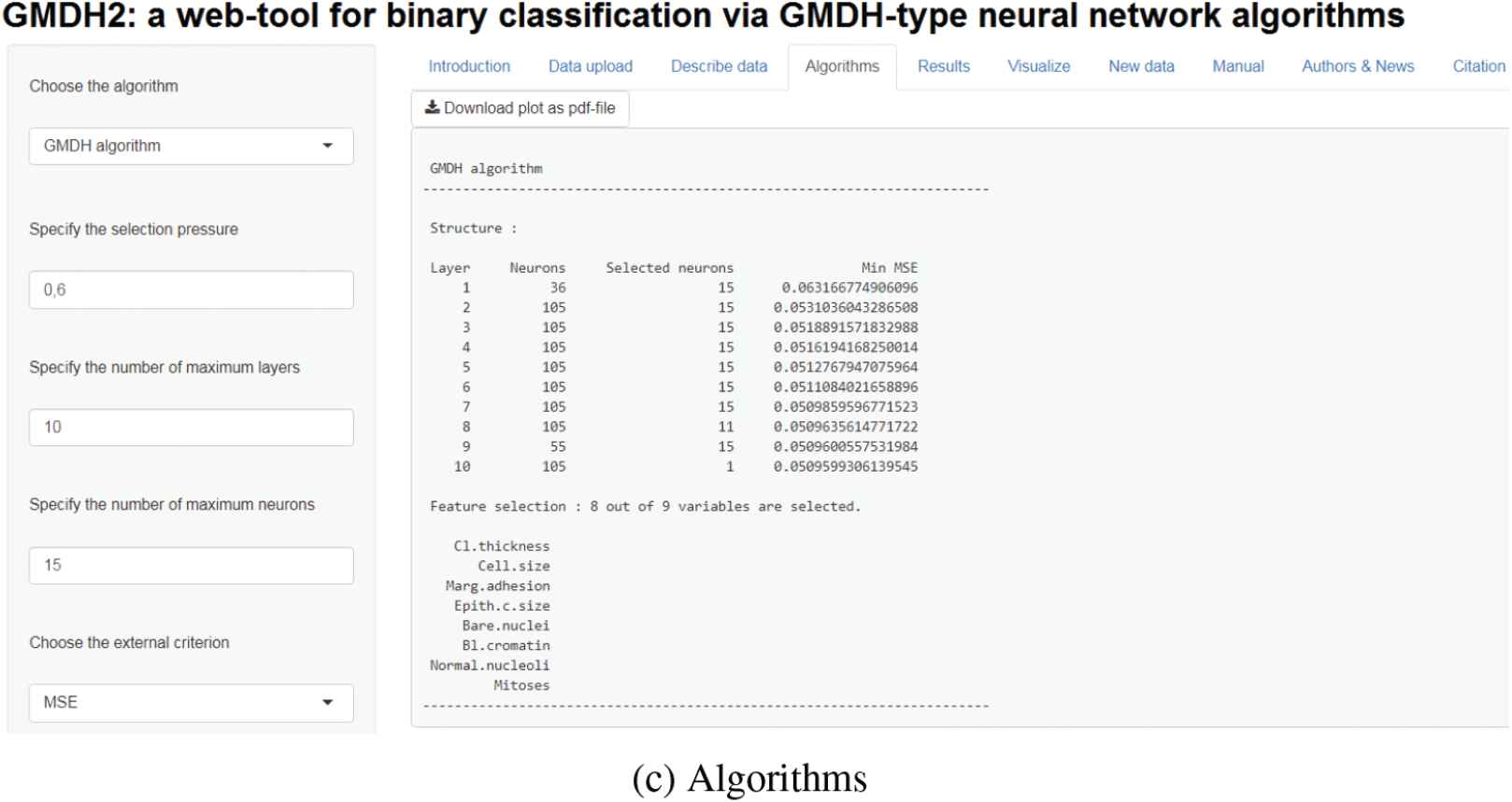
Structure :
Layer Neurons S. neurons Min MSE
1 36 15 0.06316
2 105 15 0.05310
3 105 15 0.05188
4 105 15 0.05161
5 105 15 0.05127
6 105 15 0.05110
7 105 15 0.05098
8 105 11 0.05096
9 55 15 0.05096
10 105 1 0.05095
External criterion : Mean Square Error
Feature selection : 8 out of 9
variables are selected.
Cl.thickness
Cell.size
Marg.adhesion
Epith.c.size
Bare.nuclei
Bl.cromatin
Normal.nucleoli
Mitoses
Here, the structure includes layer, neurons, s. neurons, and min MSE in the output above. The layer shows the number of layer. The neurons represent the number of neurons in corresponding layer. The s. neurons mean the number of selected neurons. The min MSE respresents the minimum external criterion which is calculated for the neuron gives the minimum external criterion on validation set in the corresponding layer. There exist two options for the external criterion namely, mean square error and mean absolute error.
Eight variables—clump thickness, uniformity of cell size, marginal adhesion, single epithelial cell size, bare nuclei, bland chromatin, normal nucleoli, mitoses—are selected by the algorithm. Minimum external criterion can be plotted across layers (presented in Figure 3) by the following code:
R> plot(model)
Predictions for test set can be made after model building process is completed. Test set has 136 observations, but only 10 of them are reported to save space.
R> predict(model, x.test, type = "class")
  [1] benign benign benign benign benign
  [6] benign malignant benign benign
  [10] benign
Levels: benign malignant
R> predict(model, x.test, type =
"probability")
            benign   malignant
  [1,] 1.000000000 0.000000000
  [2,] 0.643870382 0.356129618
  [3,] 0.670641964 0.329358036
  [4,] 0.974398179 0.025601821
  [5,] 0.920988111 0.079011889
  [6,] 0.994693987 0.005306013
  [7,] 0.436033878 0.563966122
  [8,] 0.951034736 0.048965264
  [9,] 1.000000000 0.000000000
 [10,] 0.994693987 0.005306013

Minimum external criterion across layers (GMDH algorithm).
The GMDH algorithm predicts that the probability of benign for the first and second persons are 100% and 64.4%, respectively. Since the predicted probability of benign is greater than the predicted probability of malignant, these persons are classified as benign.
3.3. Confusion Matrix and Related Statistics: confMat()
The confMat() function produces a confusion matrix for a binary response. It also returns some related statistics. These statistics are accuracy, no information rate, unweighted Kappa statistic, Matthews correlation coefficient, sensitivity, specificity, positive predictive value, negative predictive value, prevalence, balanced accuracy, youden index, detection rate, detection prevalence, precision, recall, and F1 measure. The formulation of these statistics are not stated in this paper, but presented in the manual of GMDH2 package. The positive argument is an optional character string used to specify the positive factor level. The verbose argument is utilized to print the output in R console.
# obtain predicted classes for test set
R> y.test_pred <- predict(model, x.test,
type = "class")
# obtain confusion matrix and some
statistics for test set
R> confMat(y.test_pred, y.test, positive
= "malignant")
Confusion Matrix and Statistics
           reference
data        malignant benign
  malignant        51      1
  benign            5     79
     Accuracy             :   0.9559
     No Information Rate  :   0.5882
     Kappa                :   0.9079
     Matthews Corr Coef   :   0.9097
     Sensitivity          :   0.9107
     Specificity          :   0.9875
     Positive Pred Value  :   0.9808
     Negative Pred Value  :   0.9405
     Prevalence           :   0.4118
     Balanced Accuracy    :   0.9491
     Youden Index         :   0.8982
     Detection Rate       :   0.375
     Detection Prevalence :   0.3824
     Precision            :   0.9808
     Recall               :   0.9107
     F1                   :   0.9444
     Positive Class       :   malignant
Accuracy of GMDH algorithm is estimated to be 0.9559. This algorithm classifies 95.59% of persons in a correct class. Also, sensitivity and specificity are calculated as 0.9107 and 0.9875. The algorithm classifies 91.07% of the persons having breast cancer, 98.75% of the persons not having breast cancer.
3.4. Scatter Plots with Classification Labels: cplot2d() and cplot3d()
The cplot2d() and cplot3d() functions provide interactive 2-dimensional (Figure 4a) and 3-dimensional (Figure 4b) scatter plots with classification labels, respectively. These functions originally use the plot_ly function from plotly [28] package. The first two arguments of cplot2d() are the exploratory variables stated in the x and y axes of Figure 4a. The first three arguments of cplot3d() are the exploratory variables placed in the x, y, and z axes of Figure 4b. The ypred and yobs arguments are predicted and observed classes. The colors and symbols arguments are used to specify the colors and symbols of true/false classification labels, respectively. The size of symbols can be changed with the size argument. The names of axes can be changed with the arguments xlab, ylab, zlab, and title.
# to produce 2D scatter plot with
classification labels for test set
R> cplot2d(x.test[,1], x.test[,2],
y.test_pred, y.test, colors = c("red",
"black"), xlab = "clump thickness",
ylab = "uniformity of cell size")
# to produce 3D scatter plot with
classification labels for test set
R> cplot3d(x.test[,1], x.test[,2],
x.test[,6], y.test_pred, y.test,
colors = c("red", "black"),
xlab = "clump thickness",
ylab = "uniformity of cell size",
zlab = "bare nuclei")

Scatter plots with classification labels.
3.5. Diverse Classifiers Ensemble Based on GMDH Algorithm: dceGMDH()
In this part, we demonstrate dceGMDH() function for classification. It constructs dce-GMDH algorithm, returns summary statistics of dce-GMDH architecture and assembled classifiers. Like GMDH() function, the first and second arguments are a matrix of the exploratory variables and a factor in training set, respectively. The third and fourth arguments are a matrix of the exploratory variables and a factor in validation set, respectively. The alpha argument is the selection pressure. The maxlayers argument is the specified maximum number of layers. The maxneurons argument is the maximum number of neurons allowed in the second and later layers. The exCriterion argument is the external criterion to be utilized for neuron selection. The verbose argument is utilized to print the output in R console. Also, there are the arguments for options of classifiers. The svm_options argument is a list for options of svm. The randomForest_options argument is a list for options of randomForest. The naiveBayes_options argument is a list for options of naiveBayes. The cv.glmnet_options argument is a list for options of cv.glmnet (the elastic net mixing parameter is fixed to 0.5 as default). The nnet_options argument is a list for options of nnet.
R> set.seed(seed)
# construct model via dce-GMDH algorithm
R> model <- dceGMDH(x.train, y.train,
x.valid, y.valid, alpha = 0.6, maxlayers
= 10, maxneurons = 15, exCriterion =
"MSE", verbose = TRUE)
 Structure :
 Layer   Neurons  S. neurons    Min MSE
     0         5           5    0.04669
     1        10           1    0.04641
 External criterion   : Mean Square Error
 Classifiers ensemble : 2 out of 5
 classifiers are assembled.

       svm
 cv.glmnet
In this example, two classifiers—support vector machine and elastic net logistic regression—are assembled by the algorithm. Minimum external criterion can be plotted across layers (presented in Figure 5) by the following line:
R> plot(model)

Minimum external criterion across layers (dce-GMDH algorithm).
Predictions for test set can be made after model building process is completed. Test set has 136 observations; therefore, 10 of them are reported to save space.
R> predict(model, x.test, type = "class")
  [1] benign benign malignant benign
  [5] benign benign malignant benign
  [9] benign benign
Levels: benign malignant
R> predict(model, x.test, type =
"probability")
             benign    malignant
  [1,] 0.9571287282 4.287127e-02
  [2,] 0.8317147956 1.682852e-01
  [3,] 0.3400820793 6.599179e-01
  [4,] 1.0000000000 0.000000e+00
  [5,] 0.9876416020 1.235840e-02
  [6,] 1.0000000000 0.000000e+00
  [7,] 0.2762650840 7.237349e-01
  [8,] 1.0000000000 0.000000e+00
  [9,] 1.0000000000 0.000000e+00
 [10,] 1.0000000000 0.000000e+00
The dce-GMDH algorithm predicts that the probability of benign for the first and second persons are 95.7% and 83.2%, respectively. Since the predicted probability of benign is greater than the predicted probability of malignant, these persons are classified as benign.
Confusion matrix and related statistics are obtained through the following codes to investigate the performance measures for the test set:
# obtain predicted classes for test set
R> y.test_pred <- predict(model, x.test,
type = "class")
# obtain confusion matrix and some
statistics for test set
R> confMat(y.test_pred, y.test, positive
= "malignant")
Confusion Matrix and Statistics
           reference
data        malignant benign
  malignant        54      1
  benign            2     79
     Accuracy             :   0.9779
     No Information Rate  :   0.5882
     Kappa                :   0.9543
     Matthews Corr Coef   :   0.9545
     Sensitivity          :   0.9643
     Specificity          :   0.9875
     Positive Pred Value  :   0.9818
     Negative Pred Value  :   0.9753
     Prevalence           :   0.4118
     Balanced Accuracy    :   0.9759
     Youden Index         :   0.9518
     Detection Rate       :   0.3971
     Detection Prevalence :   0.4044
     Precision            :   0.9818
     Recall               :   0.9643
     F1                   :   0.973
     Positive Class       :   malignant
Accuracy rate of dce-GMDH algorithm is estimated to be 0.9779. This algorithm classifies 97.79% of persons in a correct class.
All in all, using dce-GMDH algorithm increases the classification performance approximately 2% in accuracy compared to GMDH algorithm for this data set.
4. WEB-TOOL DEVELOPMENT
The purpose of this package is to perform binary classification via GMDH-type neural network algorithms. This package presents two main algorithms: GMDH algorithm and dce-GMDH algorithm. GMDH algorithm performs binary classification and returns the variables dominating the system. dce-GMDH algorithm performs binary classification by assembling classifiers depending on GMDH algorithm.
The package provides a well-formatted table of descriptives in different format (R, LaTeX, HTML). Also, it produces confusion matrix, its related statistics and scatter plot (2D and 3D) with classification labels of binary classes to assess the contribution of the variables on the prediction performance. It is sometimes difficult for applied researchers to deal with R codes. Therefore, a web-interface of GMDH2 package is developed by using shiny [29] package. This web-interface is available at url-http://www.softmed.hacettepe.edu.tr/GMDH2.
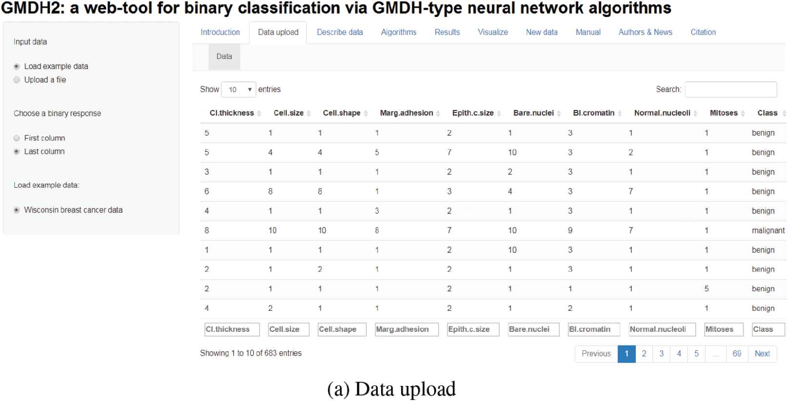
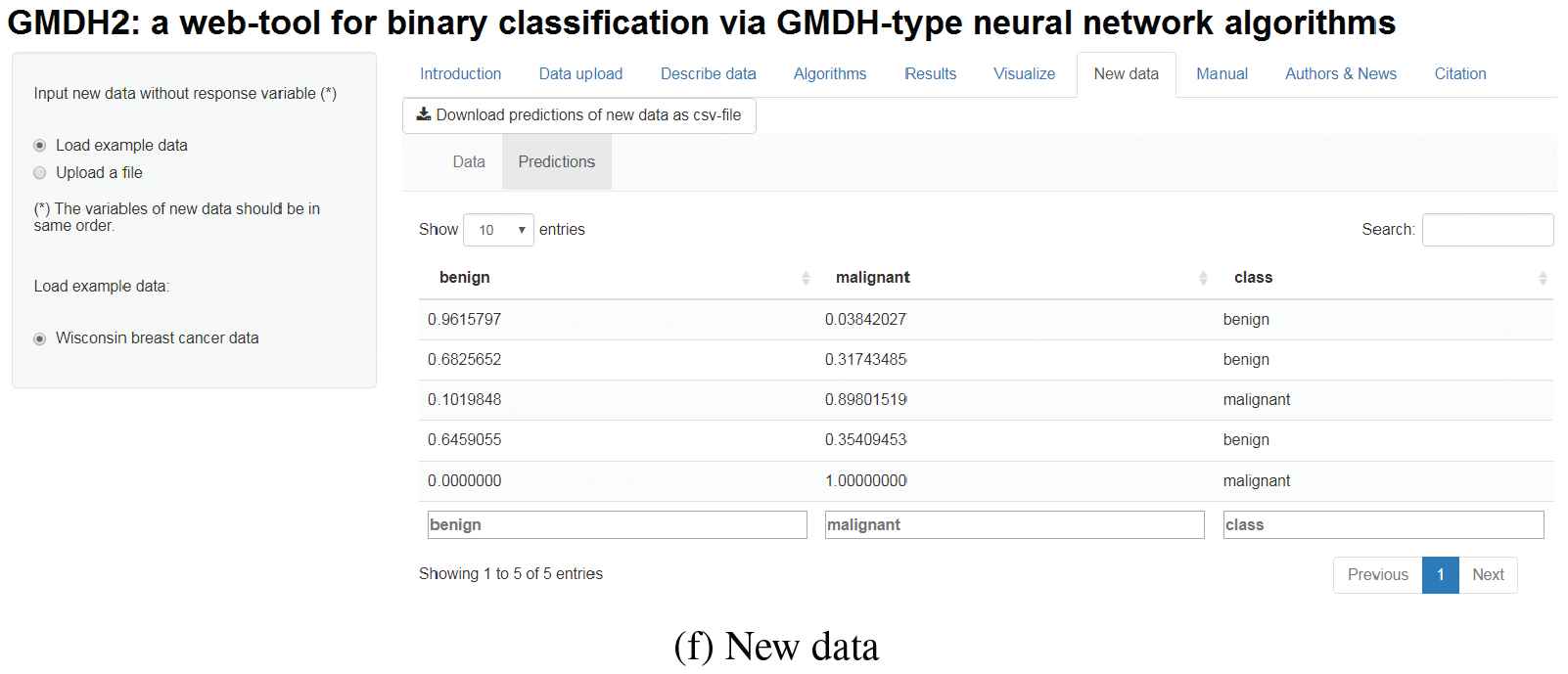
Researchers can upload their data to the tool through Data upload tab (Figure 6a). There is a demo dataset called Wisconsin breast cancer dataset on this tab for the researchers to test the tool. Basic descriptive statistics can be obtained via Describe data tab (Figure 6b). These statistics can be obtained in different formats (R, LaTeX, HTML). After describing the data, researchers can specify the algorithm desired through Algorithms tab (Figure 6c). In this tab, there exist two main algorithms: GMDH and dce-GMDH algorithms. Researchers can obtain the performance measures of classification through Results tab (Figure 6d). Moreover, predicted probabilities and classes can be downloaded via this tab. Researchers can examine the interactive scatter plots with classification labels (Figure 4) via Visualize tab (Figure 6e). At last, researchers can upload new data, obtain predicted probabilities and classes through New data tab (Figure 6f). Also, these predictions can be downloaded via this tab.


Web-tool of GMDH2 package.
5. REAL DATA APPLICATIONS
5.1. Case Study on Real Datasets
In this section, we will implement GMDH2 using several real datasets. The first data set is Wisconsin breast cancer data collected by Wolberg and Mangasarian [26]. The implementation of the package demonstrated on this data set is introduced in Section 3.
The second data set is ionosphere data downloaded from mlbench [27] R package. This data set was collected by a system in Goose Bay, Labrador. Free electrons were targeted in the ionosphere. This data set contains 351 radar returns with 34 attributes. Providing that the radar returns illustrate evidence of some type of structure in the ionosphere, they are called “good” radar returns. Otherwise, their signals pass through the ionosphere and they are called “bad” returns. There exist 225 and 126 observations in each group, respectively.
Finally, we utilized sonar data downloaded from mlbench [27] R package. Sonar signals are classified to be bounced off a metal cylinder or a roughly cylindrical rock. This data set includes 208 sonar signals (111 and 97 observations in each group, respectively) with 60 attributes. Each attribute is in the range 0.0 to 1.0. Each attribute represents the energy within a particular frequency band.
5.2. Implementation of the GMDH2 Package
We perform both GMDH and dce-GMDH classifiers on Wisconsin breast cancer data, Ionosphere data, and Sonar data. In the methods, selection pressure is set to 0.6. The maximum number of neurons is fixed to 15. The maximum number of layers is set to 10. MSE is used as an external criterion in all analyses.
The data set is split into three parts as train, validation and test sets including 60%, 20%, and 20% of all samples, respectively. In this part, the performances of the GMDH classifiers are reported based on the confusion matrices of true and predicted classes for test sets. The seed number is fixed to “12345” for the reproducibility of the results.
5.3. Performance Comparison of GMDH Classifiers
In this section, we discuss the performance of the GMDH classifiers. As it is mentioned in the earlier sections, several measures are considered for the model performances. We reported the results in Table 2 with accuracy, no information rate, Kappa, Matthews correlation coefficient, sensitivity, specificity, positive predictive value, negative predictive value, prevalence, balanced accuracy, youden index, detection rate, detection prevalence, precision, recall, and F1 measure.
| Breast Cancer | Ionosphere | Sonar | ||||
|---|---|---|---|---|---|---|
| Number of features | 9 | 34 | 60 | |||
| Number of observations | 683 | 351 | 208 | |||
| Class sizes | 239/444 | 225/126 | 111/97 | |||
| Class ratios | 0.538:1 | 1.786:1 | 1.144:1 | |||
| Train/Validation/Test | 410/137/136 | 211/70/70 | 125/42/41 | |||
| GMDH | dce-GMDH | GMDH | dce-GMDH | GMDH | dce-GMDH | |
| Accuracy | 0.9559 | 0.9779 | 0.9000 | 0.9429 | 0.7805 | 0.8049 |
| No information rate | 0.5882 | 0.5882 | 0.6857 | 0.6857 | 0.5854 | 0.5854 |
| Kappa | 0.9079 | 0.9543 | 0.7461 | 0.8641 | 0.5591 | 0.6048 |
| Matthews corr coef | 0.9097 | 0.9545 | 0.7714 | 0.8661 | 0.5653 | 0.6078 |
| Sensitivity | 0.9107 | 0.9643 | 1.0000 | 0.9792 | 0.7500 | 0.7917 |
| Specificity | 0.9875 | 0.9875 | 0.6818 | 0.8636 | 0.8235 | 0.8235 |
| Positive pred value | 0.9808 | 0.9818 | 0.8727 | 0.9400 | 0.8571 | 0.8636 |
| Negative pred value | 0.9405 | 0.9753 | 1.0000 | 0.9500 | 0.7000 | 0.7368 |
| Prevalence | 0.4118 | 0.4118 | 0.6857 | 0.6857 | 0.5854 | 0.5854 |
| Balanced accuracy | 0.9491 | 0.9759 | 0.8409 | 0.9214 | 0.7868 | 0.8076 |
| Youden index | 0.8982 | 0.9518 | 0.6818 | 0.8428 | 0.5735 | 0.6152 |
| Detection rate | 0.3750 | 0.3971 | 0.6857 | 0.6714 | 0.4390 | 0.4634 |
| Detection prevalence | 0.3824 | 0.4044 | 0.7857 | 0.7143 | 0.5122 | 0.5366 |
| Precision | 0.9808 | 0.9818 | 0.8727 | 0.9400 | 0.8571 | 0.8636 |
| Recall | 0.9107 | 0.9643 | 1.0000 | 0.9792 | 0.7500 | 0.7917 |
| F1 | 0.9444 | 0.9730 | 0.9320 | 0.9592 | 0.8000 | 0.8261 |
GMDH, group method of data handling; dce-GMDH, diverse classifiers ensemble based on group method of data handling.
Classification results for real datasets.
According to the measures of accuracy, kappa, Matthews correlation coefficient, positive predictive value (precision), balanced accuracy, youden index and F1, dce-GMDH algorithm is superior to GMDH algorithm in all data sets. With respect to sensitivity (recall) and negative predictive value, dce-GMDH algorithm performs better compared to GMDH algorithm on both breast cancer and sonar data sets, but vice versa is true on ionosphere data set. According to the measure of specificity, dce-GMDH classifier performs as well as GMDH classifier except for ionosphere data, but it performs better than GMDH classifier on ionosphere data.
6. SUMMARY AND FURTHER RESEARCH
Binary classification is a problem in which binary factor labels can be predicted for each observation. Binary classification is used in different disciplines. Examples include medical studies, economics, agriculture, meteorology, and so on. In this paper, we present GMDH2 package to perform binary classification through GMDH-type neural network algorithms.
The GMDH2 package offers two main algorithms; namely, GMDH and dce-GMDH algorithms. GMDH algorithm makes binary classification and determines which features are important for discrimination of classes. dce-GMDH algorithm assembles the classifiers—support vector machines, random forest, naive Bayes, elastic net logistic regression, artificial neural network—based on GMDH algorithm to perform classification for a binary response. Moreover, the package provides a table of descriptives for a binary factor in different formats (R, LaTeX, HTML). The package also produces confusion matrix, its related statistics, and scatter plot (2D and 3D) with classification labels of binary classes to assess the prediction performance. The package and its web-interface will be updated regularly.
Future studies are planned in the direction of multi-label classification. Moreover, these algorithms can be used for the large number of variables, such as classification of genomics data. With especially GMDH algorithm, selection of important genes can be conducted.
CONFLICT OF INTEREST
The authors declare there is no conflict of interest.
AUTHORS' CONTRIBUTIONS
Osman Dag conceived and designed the study, performed the study, developed the R package and its web-based tool, analyzed the data sets, wrote the paper, prepared figures and table(s).
Erdem Karabulut and Reha Alpar conceived and designed the study, wrote the paper, reviewed drafts of the paper.
Funding Statement
This study is supported by 2211/A Scholarship Program within The Scientific and Technological Research Council of Turkey and by Hacettepe University Scientific Research Projects Coordination Unit with project Number THD-2018-16610.
ACKNOWLEDGMENTS
We thank the anonymous reviewers for their constructive comments and suggestions which helped us to improve the quality of our paper. This study is supported by 2211/A Scholarship Program within The Scientific and Technological Research Council of Turkey and by Hacettepe University Scientific Research Projects Coordination Unit with project Number THD-2018-16610.
REFERENCES
Cite this article
TY  - JOUR
AU  - Osman Dag
AU  - Erdem Karabulut
AU  - Reha Alpar
PY  - 2019
DA  - 2019/06/17
TI  - GMDH2: Binary Classification via GMDH-Type Neural Network Algorithms—R Package and Web-Based Tool
JO  - International Journal of Computational Intelligence Systems
SP  - 649
EP  - 660
VL  - 12
IS  - 2
SN  - 1875-6883
UR  - https://doi.org/10.2991/ijcis.d.190618.001
DO  - 10.2991/ijcis.d.190618.001
ID  - Dag2019
ER  -