
A Real-Coded Optimal Sensor Deployment Scheme for Wireless Sensor Networks Based on the Social Spider Optimization Algorithm
- DOI
- 10.2991/ijcis.d.190614.001How to use a DOI?
- Keywords
- Wireless sensor networks; Optimal sensor deployment; Social Spider Optimization; Metaheuristics
- Abstract
Wireless sensor networks (WSNs) involves a set of wireless sensor nodes located within a region of interest (ROI) to acquire and/or transmit specific information from their surroundings. A common problem in the operation of WSNs is sensor coverage, which is related to the distribution of sensor nodes within their ROI. Several approaches have been proposed to solve this problem; however, most of these methods consider a simplified arrangement scheme based on sensor placement over a set of fixed discrete locations defined by a grid. This fact severally limits the ability of these methods to find potentially better solutions as they are conditioned to select a limited number of candidate solutions. In this paper, a real-coded sensor deployment approach based on the Social Spider Optimization (SSO) algorithm is proposed to solve the problem of optimal sensor deployment (OSD) in WSNs. The performance of our proposed approach (referred in this paper as real-coded SSO [R-SSO]) was also compared against other metaheuristics-based methods used in the literature. Experimental results demonstrate its ability to solve the problem of OSD in terms of accuracy and robustness.
- Copyright
- © 2019 The Authors. Published by Atlantis Press SARL.
- Open Access
- This is an open access article distributed under the CC BY-NC 4.0 license (http://creativecommons.org/licenses/by-nc/4.0/).
1. INTRODUCTION
The development of wireless communication technologies has led to a rapid increase in the use of wireless sensor networks (WSNs) for a vast number of applications, ranging from civilian to military [1]. WSNs consists of a set of wireless sensor devices (or sensor nodes) located within a specific region of interest (ROI) with the intention of acquiring or transmitting information from their surroundings [2–7]. Each sensor node is capable of sensing and processing data (see Figure 1). Furthermore, sensor nodes also have communication capabilities, which allow them to transmit and share information with other sensing units within the WSN. Nowadays, WSNs are relevant for many application domains, which include vehicular tracking, seismic activity observation, forest monitoring, target detection, and surveillance, among others [1].
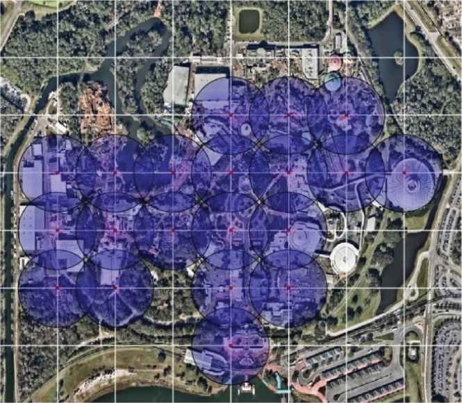
Wireless Sensor Network composed of 20 sensor nodes (red dots), deployed for the monitoring of some specific data within several regions of interest in an amusement park. The coverage radius of each sensor (blue circles) is shown for illustrative purposes.
Sensor coverage is one of the most studied problems related to the operation of WSN. In sensor coverage, the idea is to find the spatial configuration of sensor nodes within a given ROI so that the WSN reaches the best possible coverage of the ROI. In the design of a WSN, for practical reasons, it is common to distribute sensor nodes randomly.
However, this method does not guarantee sufficient coverage of the ROI, especially when sensors nodes adopt a configuration with small concentrations in specific locations of the service area. Since the coverage performance of a WSN depends on the spatial arrangement of the sensor nodes, techniques to properly distribute sensor nodes had been extensively studied and developed in the last few years; as a result, there are plenty of works on the literature devoted to this subject [8–16].
Recently, due to interesting results, the use of metaheuristic optimization techniques have received increasing attention as an alternative to solve the optimal sensor deployment (OSD) for WSNs. Some approaches include schemes such as the Self-Deployment method based on the implementation of the Virtual Force Algorithm (VFA) [7]. This scheme was proposed to improve sensor field coverage via the reconfiguration of randomly placed sensing units into uniformly distributed node topologies. Similarly, in [17], a sensor deployment approach based in Particle Swarm Optimization (PSO) has been applied with the objective to maximize sensor coverage over a given ROI, while also considering the minimization of energy usage in cluster-based network topologies. Also, in [18], a multiobjective implementation of Genetic Algorithms (GAs) [18] has been employed to optimize the configuration of WSNs with regard to two competing objectives: sensor coverage and network's lifetime. Furthermore [19], proposes a sensor deployment scheme based on a recent swarm optimization algorithm known as Social Spider Optimization (SSO). In this scheme, a simple binary sensor coverage model is implemented as part of the primary optimization criterion, yielding to good results. Although the previous sensor deployment approaches have demonstrated to produce competitive results, these methods often model the deployment area as a discrete grid, which for most cases comprises an unrealistic assumption. Under such conditions, the lattice presents a finite number of positions (grid points) in which sensor nodes can be placed. Intuitively, such assumption limits the flexibility of the sensor distribution approach, as it restricts the deployment of candidate locations to those modeled in the grid.
In this paper, we propose an SSO-based approach for OSD in WSNs. In our proposed method, the SSO algorithm is applied with the intention of finding an optimal arrangement for a set of available sensor nodes (that is, a configuration that enables to maximize the area covered by the sensor network). However, different to previous works on the literature which consider only a set of candidate positions defined by a 2-D grid, our approach considers the deployment area to be defined as a continuous flat surface; as such, instead of only considering a set of finite positions as candidate for placing a sensor node, our approach is able to place sensing devices in virtually any real location within the ROI. Also, instead of calculating the number of grid points that are covered by the deployed WSN, the total covered area is estimated by considering the intersection between the individual coverage area of each sensor node. Under these considerations, our proposed approach is able to handle some technical challenges related to optimal WSN deployment: first of all, considering real candidate locations instead of a set of finite discrete locations gives our proposed method the flexibility to explore potentially better solutions to the sensor deployment problem, while also increasing its performance when placement restrictions are introduced; in second place, the fact that the actual covered area is considered for calculating the coverage area rate allows to reduce the uncertainty of the model, as this gives us better insight on the actual amount of the ROI that is being monitored by the sensor network under certain arrangement configurations.
Our proposed approach has been exhaustively tested and compared with other similar methods. The experimental results reported in this work are presented three stages: first, we present a comparison between discrete-coded and real-coded OSD schemes based SSO; furthermore, we include an exhaustive comparison against different real-coded OSD approaches based on other popular metaheuristic optimization techniques such as Moth-flame Optimization (MFO) algorithm [20], Firefly Algorithm (FA) [21], PSO [22], Artificial Bee Colony (ABC) [23], Whale Optimization Algorithm (WOA) [24], Crow Search Algorithm (CSA) [25], and Grey Wolf Optimizer (GWO) [26]; finally, a comparison of these techniques with regard to a particular case of OSD, which involves the deployment of a set of sensor nodes within several specific disjointed ROIs.
The rest of this paper is organized as follows: in Section 2, we discuss some approaches commonly applied for calculating the rate of coverage in WSNs. In Section 3, we review the SSO algorithm, highlighting its main characteristics and steps. In Section 4, we describe our proposed SSO-based OSD approach, emphasizing its differences to previously proposed similar methods. In Section 5, we present our comparative analysis and results for the three previously specified sets of experiments. Finally, in Section 6, we present our conclusions for this work.
2. OSD FOR WSNs
WSNs consist of multiple sensors distributed through a specified sensing area with the purpose of acquiring some physical or environmental data. The main problem regarding the deployment of WSNs is the optimal placement of sensor nodes along a specified service area so that the resulting sensor network achieve sufficient coverage (i.e., that each location within the service area is monitored by at least one sensor unit). One of the most common models applied for OSD in WSNs is represented by the binary sensor model (BSM). According to this scheme, the coverage probability for any given position
For simplicity, most sensor deployment schemes assume that the experimental environment is represented by a 2-D grid
By considering the previous, the total area covered by the set of deployed sensor nodes may be given by adding up the coverage probabilities for all locations within the modeled 2-D grid; this is
Finally, the deployment area's coverage rate is calculated by
3. SOCIAL SPIDER OPTIMIZATION
The SSO algorithm is a swarm intelligence approach proposed by Cuevas et al. in 2013. As its name implies, the SSO approach draws inspiration on the collective behaviors manifested by certain species of spiders known for living in social units or colonies [27–30]. In nature, social spider colonies are mainly composed by two components: its members, which may be further distinguished by their gender (male or female), and a communal web which serves as a medium for interaction and communication among its inhabitants. Depending on their gender and particular characteristics, each member of the colony is assigned to cooperate in several activities, including building and maintaining the communal web, capturing prey, mating, and so on. Another interesting trait related to Social Spiders lies on their capacity to perceive the vibrations transmitted through the communal web. Each member on the colony can translate these vibrations into important information related to their surroundings, including the location and size of both, neighboring members and prey trapped in the communal web.
3.1. Main Operators of the SSO Algorithm
In the SSO approach, search agents are modeled as individual spiders, whose positions
Furthermore, the SSO approach considers the gender of spiders (either male or female) as part of its search strategy. With that being said, the initial population
Furthermore, spiders within the communal web are assumed to be able to communicate with each other through a series of vibrations, emitted by each of them and transmitted through the silk threads which comprise said communal area. In the SSO approach, the vibration perceived by a given spider ‘i’ as a result of the information transmitted by a different spider ‘j’ is modeled as follows:

Vibration models in the Social Spider Optimization (SSO) algorithm: (a) Vibci, (b) Vibbi and (c) Vibfi.
The vibrations
The vibrations
The vibrations
Also, depending on their gender, spiders are assumed to be able to manifest several different behaviors. In the case of female spiders, for example, an attraction or dislike toward other members of the colony (independent of their gender) may be manifested. In the SSO approach, such a phenomenon is modeled as either an attraction or repulsion movement toward other prominent individuals within the communal web. With that being said, at each iteration “
On the other hand, male spiders, which are said to manifest an exclusive attraction toward female individuals within the communal web, may be further identified as either dominant or nondominant male spiders. Typically, dominant male spiders have more prominent characteristics (i.e., a greater size or weight) in comparison to nondominant male spiders. Furthermore, while dominant male spiders are usually attracted toward their closest female spider in the communal web, nondominant male spiders tend to concentrate toward the center of the male population as a strategy to take advantage of resources that are wasted by dominant males. In SSO, these male-characteristic behaviors are modeled by first considering the median weight from within the group of male spiders. At each iteration “
Finally, the SSO approach employs a mating mechanism in which female spiders and dominant male spiders are used to construct new candidate solutions. For such a procedure, a dominant male spider (individual with a weight greater than the median weight value of the male population) is first selected, and then, a set of female spiders within a particular mating radius
For the mating operation, a new individual
Once these influence probabilities have been calculated, each of the elements
3.2. Computational Procedure of the SSO Algorithm
In Figure 3, we present a flowchart illustrating the main steps of the SSO algorithm [27]. In general, the computational procedure of the SSO algorithm can be summarized as follows:
Step 1 Considering
Step 2 Initialize the population of spiders (see Equations (6) and (7)).
Step 3 Calculate the weights for all spiders in the population (see Equation (9))
Step 4 Apply movement operator for female spiders (see Equation (13)).
Step 5 Apply movement operator for male spiders (see Equation (14)).
Step 6 Perform mating operation
Step 7 If the stop criterion is met, end the process; otherwise, return to Step 3.

Flowchart illustrating the computational procedure of the Social Spider Optimization (SSO) algorithm.
3.3. Computational Complexity of the SSO Algorithm
The SSO algorithm is comprised by several operators including: 1. Position update operators for both, female and male spiders; 2. Mating operator; and 3. Survival operator. Independent of their function within the SSO algorithm, the computational complexity added by any of these operators is related to the maximum number of iterations
In the case of the movement operators modeled in SSO, female and male individuals (spiders) simulate movements that are different enough between them, and also have different time complexity. This computational complexity depends on both, the size of the female population
On the other hand, the mating operation in the SSO algorithm the computational complexity is usually not fixed. In the worst-case scenario, the time complexity depends on the population sizes of female spiders (
Finally, there is the survival operation, which depends only on the number of offspring spiders
Usually, the time complexity of an algorithm as a whole can be reduced to that of its most complex procedure, disregarding all other steps [31]. As the computational complexity for the movement operators is clearly the greatest, the time complexity of the SSO algorithm can then be approximated simply as:
4. REAL-CODED SSO-BASED SENSOR DEPLOYMENT SCHEME FOR WSNs
As exposed in Section 2, the main objective behind the deployment of a WSNs is to maximize the sensor network's coverage area by choosing optimal locations within a given ROI for a set of available sensor nodes. For simplicity it is often considered that the service area has a finite amount of candidate locations where sensor nodes can be placed, commonly represented by a 2-D grid. Under this approach, the measure of how good a given sensor arrangement is may be given by its coverage area rate, which is related to the amount of locations of the modeled lattice that are covered by the sensor network. On the literature, the BSM is commonly applied in order to determine whether or not a given location
In [19], the authors proposed a sensor deployment scheme based on the SSO algorithm, in which optimal locations for a set of sensor nodes
Guided by the SSO's cooperative behavior operators, each spider
While the SSO algorithm has demonstrated competent results when applied to solve such a challenging combinatorial optimization problem, it is worth noting that the discrete nature of these sensor deployment models somewhat restricts the ability of the SSO to find potentially better placement configurations for the available sensing devices. Motivated by this fact, in this paper, a real-coded implementation based on the SSO algorithm is proposed to solve the problem of OSD in WSNs. Different to previous works, where the sensor's deployment area is modeled by a discrete grid
As previously mentioned, the key difference between our proposed approach and the one presented in [19] is the fact that in the former each available sensor node
Similar to the approach presented in [19], a BSM has been considered for the calculation of the sensor network's coverage area. The main difference, however, is that instead of calculating the covered area by counting the number of discrete locations that are covered by the sensor network, our proposed approach calculates the actual area that is covered by a given sensor deployment configuration. For this purpose, it is considered that the covered area

Flowchart illustrating the computational procedure for the proposed real-coded Social Spider Optimization (R-SSO) optimal sensor deployment (OSD) approach.
5. EXPERIMENTAL SETUP AND RESULTS
In this paper, a real-coded SSO (R-SSO)-based sensor deployment scheme is proposed for solving the problem of optimal placement of sensor nodes in WSNs. Different to other similar approaches currently reported on the literature, where the arrangement of sensor nodes is performed by considering a set of discrete positions modeled by a 2-D mesh grid, our proposed method considers a continuous experimental environment, where such sensing devices can adopt virtually any real position. As a result of this, our proposed OSD approach is able to explore a much wider set of candidate solutions, allowing it to find potentially better solutions in comparison to those provided by discrete-coded methods. In order to evaluate the performance of our proposed OSD approach, a series of comparative experiments against other similar techniques were performed. Our experimental results are divided into two parts: in Section 5.1, we present a comparative analysis between our proposed R-SSO-based approach and the discrete-coded SSO (D-SSO)-based implementation proposed in [19]; furthermore, in Section 5.2, we compare the performance of our proposed method with that of other similar techniques modified to work with real-coded positions, such as the MFO algorithm [20], FA [21], PSO [22], ABC [23], WOA [24], CSA [25], and GWO [26]; finally, in Section 5.3., additional comparative experiments, which consider the task of covering several disjointed regions of interest (ROIs) within a given service area are presented.
5.1. R-SSO-Based OSD VS D-SSO-Based OSD
Our first set of experiments involves a comparison between our proposed R-SSO-based OSD approach and the D-SSO-based OSD implementation proposed in [19]. As previously stated, the key difference between both of the compared approaches is that in the former the locations
For each experimental run, it is considered that there is an experimental environment with an area size of
| R-SSO | D-SSO | |
|---|---|---|
| 0.8436 | 0.8419 | |
| 0.8459 | 0.8418 | |
| 0.0087 | 0.0057 | |
| 0.8243 | 0.8321 | |
| 0.8553 | 0.8553 |
OSD, optimal sensor deployment; D-SSO, discrete-coded Social Spider Optimization; R-SSO, real-coded Social Spider Optimization.
Optimization results for R-SSO and D-SSO applied for the OSD of Nsensors = 20 sensor nodes (each with a coverage radius rs = 90) within an experimental environment with an area size of A = 800 × 700. The statistical results correspond to 30 individual runs per method, each by considering a population size of Npop = 50 individuals, and a maximum number of iterations of kmax = 100 as stop criterion.
Furthermore, Figure 5 presents the convergence curves corresponding to the averaged performance over the set of experimental runs of each of the compared techniques. As illustrated by the curves, the R-SSO algorithm demonstrates to have better convergence rate than his counterpart, with D-SSO manifesting a comparable performance (though still inferior when compared to R-SSO). R-SSO achieves a better fitness it each stage of the iterations.
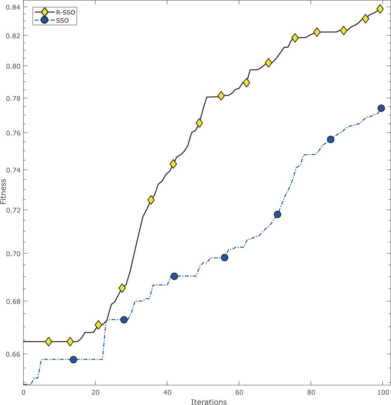
Convergence curves obtained by real-coded Social Spider Optimization (R-SSO) and discrete-coded SSO (D-SSO) when applied to solve the proposed optimal sensor deployment (OSD) problem (with A = 800 × 700, Nsensors = 20 and rs = 90). The shown curves correspond to the averaged performance over each set of experimental runs. For all cases, a population size of Npop = 50 individuals and a maximum number of iterations of kmax = 100 are considered.
Finally, in Figures 6 through 8, we show an example of an initial arrangement of sensor positions as well as the best sensor deployment configurations achieved by each of the compared methods from among their respective sets of experimental runs.
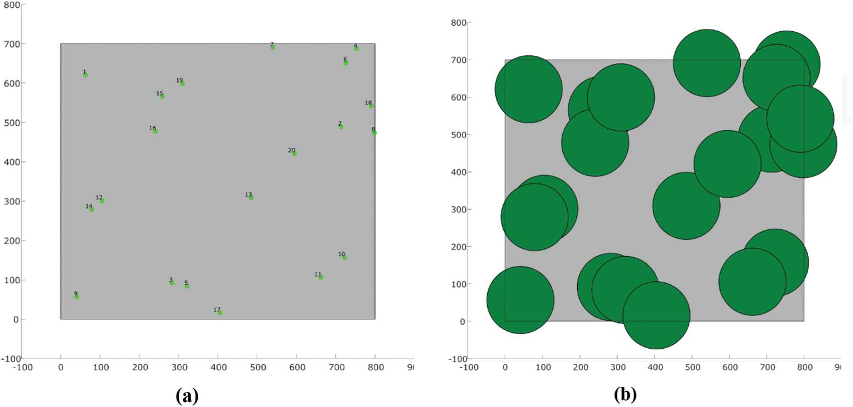
Initial sensor positions for a set of 20 sensor nodes within an experimental environment of area size A = 800 × 700: (a) sensor nodes locations and (b) area covered by the sensing devices on their initial locations.

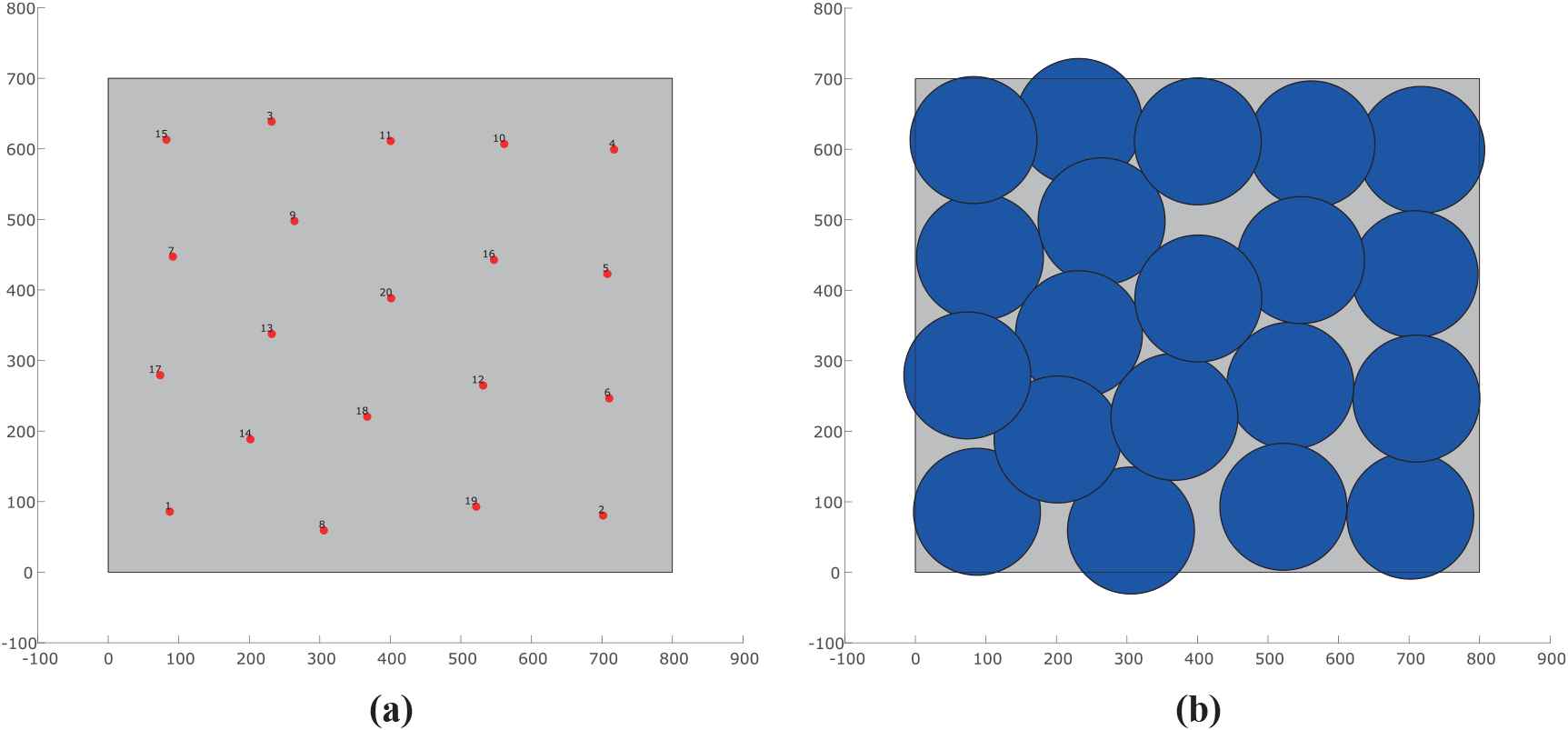
Sensor deployment configuration for 20 sensor nodes, obtained by applying the real-coded Social Spider Optimization (R-SSO) approach: (a) sensor nodes locations and (b) area covered by the deployed sensing devices.
Sensor deployment configuration for 20 sensor nodes, obtained by applying the discrete-coded Social Spider Optimization (D-SSO) approach: (a) sensor nodes locations and (b) area covered by the deployed sensing devices.
5.2. Comparison with Other Real-Coded OSD Approaches Based on Metaheuristics
To further demonstrate the performance of the proposed R-SSO-based OSD, a set of comparative experiments against some other similar techniques, modified to work with real-coded positions, is presented. Specifically, methods based on metaheuristic optimization algorithms such as MFO algorithm [20], FA [21], PSO [22], ABC [23], WOA [24], CSA [25], and GWO [26] were considered to perform our comparative experiments. The parameter setup considered for each of these algorithms is as follows:
R-SSO: The female attraction probability parameter is set as
MFO: The number of flames is set as
FA: The parameters setup for the randomness factor and the light absorption coefficient are set to
PSO: The cognitive and social coefficients are set to
ABC: The algorithm was implemented by setting the parameter limit = num Of Food Sources * dims, where num Of Food Sources = N (population size) and dims = d (dimensionality of the solution space) [23].
WOA: The internal parameters
CSA: The awareness probability is set to
GWO: The algorithm's parameter
The previously illustrated sets of parameters were determined through exhaustive experimentation; thus, these sets of parameters represent the best possible configurations for each of the compared methods. All of the compared methods were tested by considering a population size of
Our experiments aim to compare the performance of R-SSO against those of MFO, FA, PSO, ABC, CSA, WOA, and GWO when applied for the task of OSD in WSNs. Similarly to the experiments reported in Section 5.1, we consider an experimental environment with an area size of
| R-SSO | MFO | FA | PSO | CSA | ABC | WOA | GWO | |
|---|---|---|---|---|---|---|---|---|
| 0.9804 | 0.9656 | 0.9504 | 0.9417 | 0.8016 | 0.7867 | 0.9090 | 0.9593 | |
| 0.9831 | 0.9673 | 0.9514 | 0.9459 | 0.8029 | 0.7815 | 0.9078 | 0.9607 | |
| 0.0081 | 0.0104 | 0.0119 | 0.0176 | 0.0115 | 0.0177 | 0.0113 | 0.0082 | |
| 0.9586 | 0.9388 | 0.9102 | 0.9028 | 0.7864 | 0.7582 | 0.8873 | 0.9404 | |
| 0.9908 | 0.9773 | 0.9647 | 0.9637 | 0.8217 | 0.8266 | 0.9308 | 0.9769 |
ABC, Artificial Bee Colony; CSA, Crow Search Algorithm; FA, Firefly Algorithm; GWO, Grey Wolf Optimizer; MFO, Moth-flame Optimization; OSD, optimal sensor deployment; PSO, Particle Swarm Optimization; ROI, regions of interest; R-SSO, real-coded Social Spider Optimization; WOA, Whale Optimization Algorithm.
Optimization results for R-SSO, MFO, FA, PSO, CSA, ABC, WOA, and GWO for the OSD of Nsensors = 30 sensor nodes (each with a coverage radius rs = 90) within an experimental environment of size A = 800 × 700. The statistical results correspond to 30 individual runs per method, each by considering a population size of Npop = 50 individuals, and a maximum number of iterations of kmax = 300 as stop criterion.
Furthermore, Figure 9 presents the convergence curves corresponding to the averaged performance over the set of experimental runs of each of the compared techniques. As illustrated by these curves, the R-SSO algorithm demonstrates to have better convergence rate than all methods, with MFO manifesting a comparable performance (though still inferior when compared to R-SSO). Interestingly, while R-SSO, MFO, FA, PSO, and GWO seem to exhibit continuous convergence toward the global best solution, methods such as ABC, CSA, and WOA seem to have notorious difficulties to handle the proposed OSD problem, with each of them suffering from stagnation even at the earliest stages of their search process.
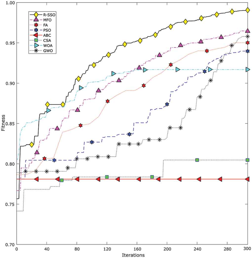
Evolution curves obtained by real-coded Social Spider Optimization (R-SSO), Moth-flame Optimization (MFO), Firefly Algorithm (FA), Particle Swarm Optimization (PSO), Artificial Bee Colony (ABC), Crow Search Algorithm (CSA), Whale Optimization Algorithm (WOA), and Grey Wolf Optimizer (GWO) when applied to solve the proposed optimal sensor deployment (OSD) problem (with A = 800 × 700, Nsensors = 30 and rs = 90). The shown curves correspond to the averaged performance over each set of experimental runs. For all cases, a population size of Npop = 50 individuals and a maximum number of iterations of kmax = 300 are considered.
Finally, in Figures 10 through 18, we show an example of an initial arrangement of sensor positions as well as the best sensor deployment configurations achieved by applying R-SSO, MFO, FA, PSO, CSA, ABC, WOA, and GWO to said initial set of positions. As evidenced by these graphical results, R-SSO can achieve a much uniform distribution of sensor nodes, while also allowing it to cover the most area when compared to the other applied methods.

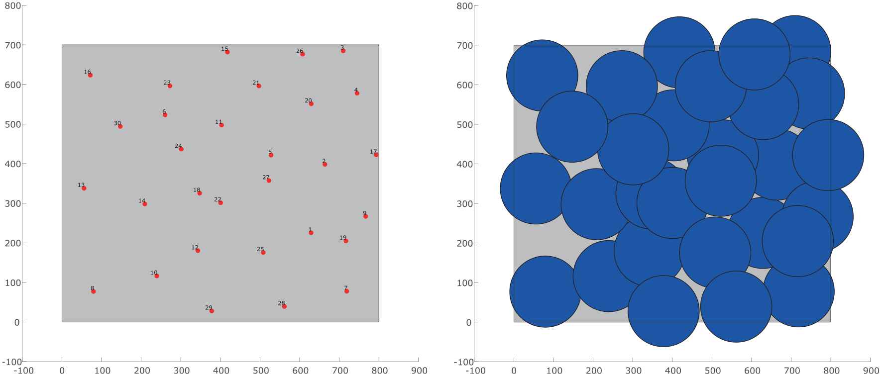
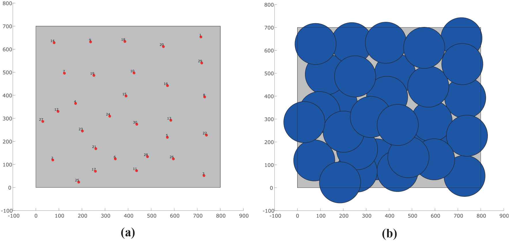
Initial configuration of positions for a set of 30 sensor nodes within an experimental environment of area size A = 800 × 700: (a) sensor nodes locations and (b) area covered by the sensing devices on their initial positions.

Sensor deployment configuration for 20 sensor nodes, obtained by applying the real-coded Social Spider Optimization (R-SSO) approach: (a) sensor nodes locations and (b) area covered by the deployed sensing devices.

Sensor deployment configuration for 20 sensor nodes, obtained by applying the Moth-flame Optimization (MFO) approach: (a) sensor nodes locations and (b) area covered by the deployed sensing devices.
Sensor deployment configuration for 20 sensor nodes, obtained by applying the Firefly Algorithm (FA) approach: (a) sensor nodes locations and (b) area covered by the deployed sensing devices.

Sensor deployment configuration for 20 sensor nodes, obtained by applying the Particle Swarm Optimization (PSO) approach: (a) sensor nodes locations and (b) area covered by the deployed sensing devices.
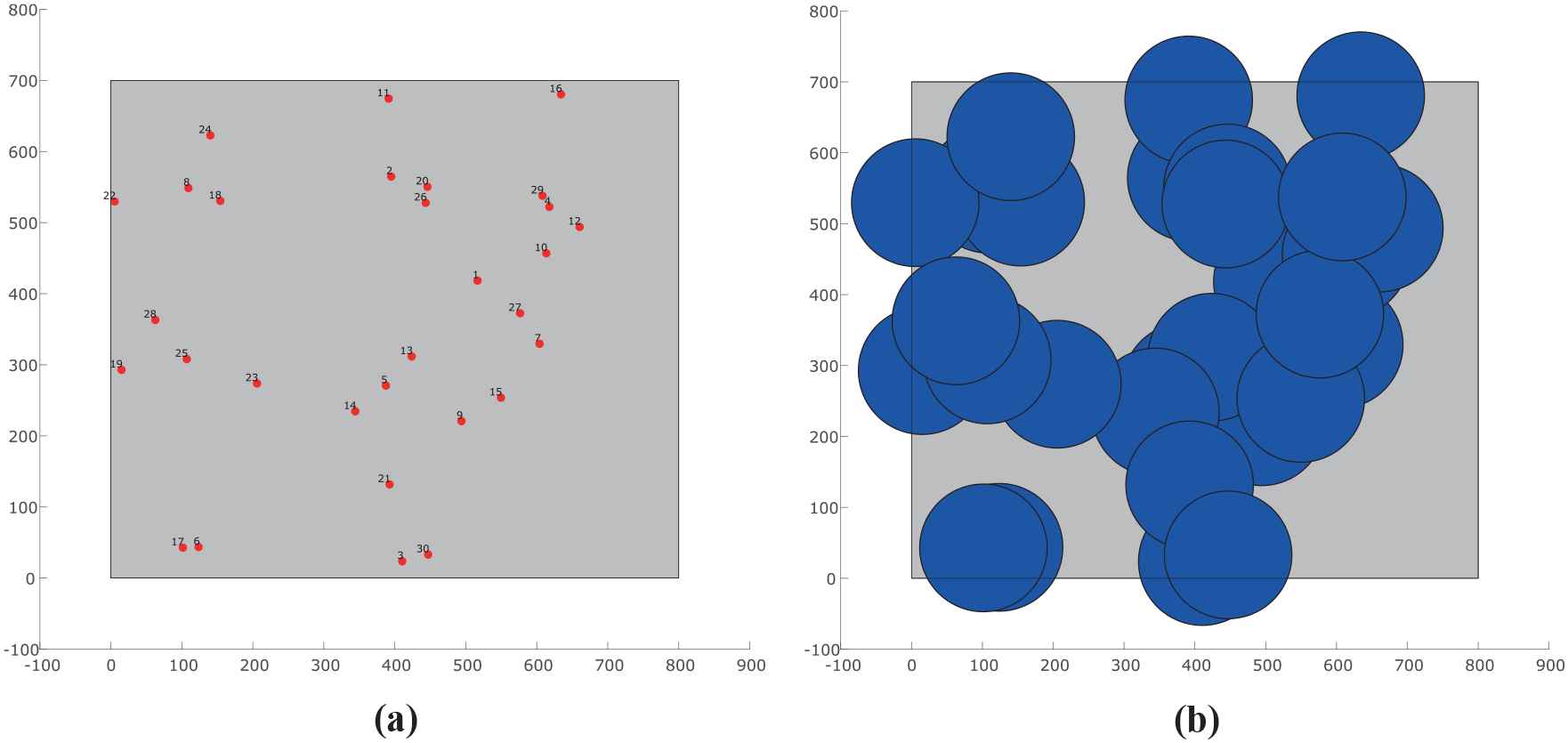
Sensor deployment configuration for 20 sensor nodes, obtained by applying the Crow Search Algorithm (CSA) approach: (a) sensor nodes locations and (b) area covered by the deployed sensing devices.

Sensor deployment configuration for 20 sensor nodes, obtained by applying the Artificial Bee Colony (ABC) approach: (a) sensor nodes locations and (b) area covered by the deployed sensing devices.
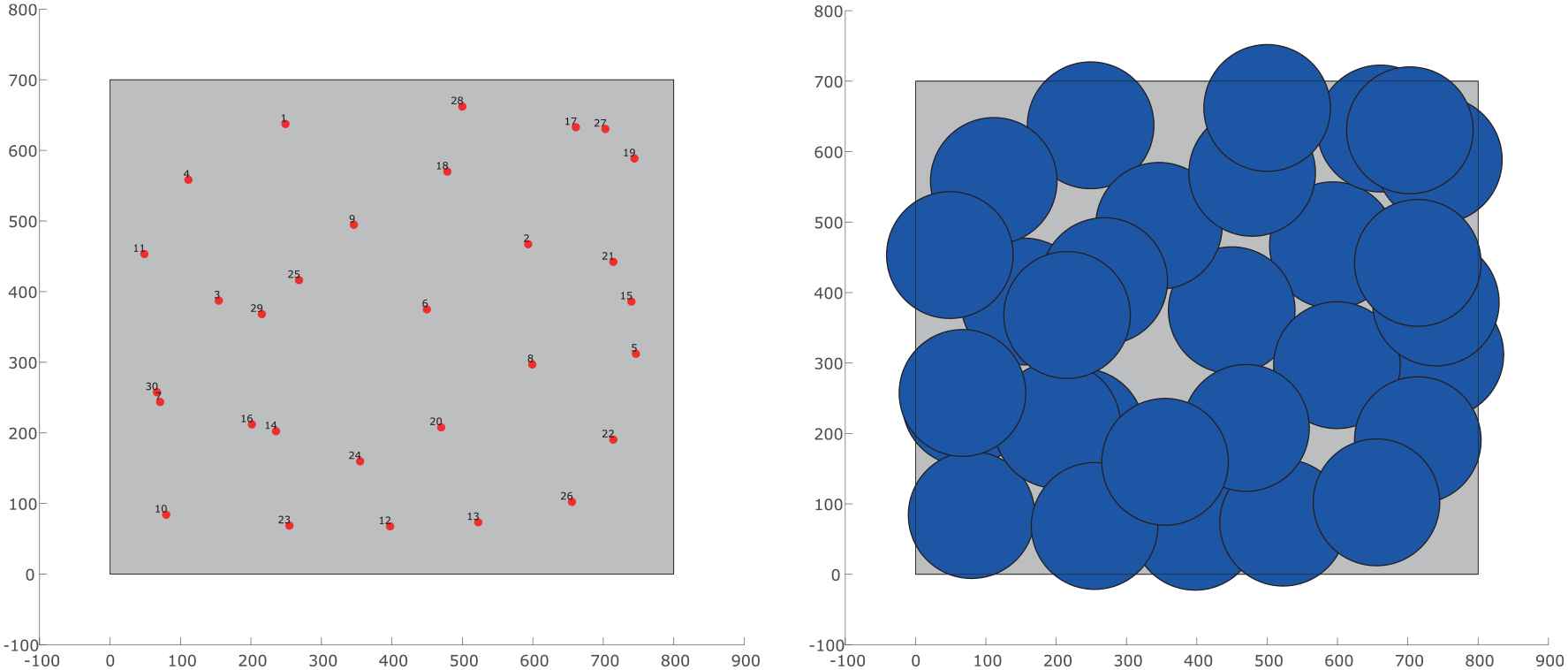
Sensor deployment configuration for 20 sensor nodes, obtained by applying the Whale Optimization Algorithm (WOA) approach: (a) sensor nodes locations, and (b) area covered by the deployed sensing devices.
Sensor deployment configuration for 20 sensor nodes, obtained by applying the Grey Wolf Optimizer (GWO) approach: (a) sensor nodes locations and (b) area covered by the deployed sensing devices.
5.3. R-SSO for OSD within a Set of Disjointed ROIs
In order to further demonstrate the capabilities of the proposed R-SSO-based OSD approach, we have formulated an additional set of experiments which involve the optimal placement of sensor nodes within several disjointed ROIs within a given experimental environment. Specifically, it is considered that an experimental environment of size of

Comparison of experimental environments of optimal sensor deployment (OSD): (a) experimental environment of area size, where here the objective is to maximize the area covered by a set of sensor nodes deployed within said service area; and (b) experimental environment with four disjointed regions of interest (ROIs) (shapes colored white), were the area that is required to be covered by the set of sensor nodes is that which is delimited by each ROIs.
Similar to the experiments reported in the previous section, the objective is to compare the performance of R-SSO against those of MFO, FA, PSO, ABC, CSA, WOA, and GWO when applied for this specific OSD case; with that being said, and for the sake of consistency, the parameter setup applied to each algorithm is kept as reported in Section 5.2. All of the compared methods were tested by considering a population size of
The experimental results, corresponding to 30 individual runs for each of the considered methods are shown in Table 3, where the best outcomes appear in boldface. As in the results reported in Section 5.2, the analyzed performance indexes correspond to the mean, median, and standard deviation of the best fitness values (
| SSO | MFO | FA | PSO | CSA | ABC | WOA | GWO | |
|---|---|---|---|---|---|---|---|---|
| 0.9923 | 0.9803 | 0.9753 | 0.9629 | 0.8003 | 0.7369 | 0.8965 | 0.9771 | |
| 0.9948 | 0.9861 | 0.9749 | 0.9728 | 0.8012 | 0.7274 | 0.9043 | 0.9763 | |
| 0.0083 | 0.0184 | 0.0086 | 0.0273 | 0.0239 | 0.0300 | 0.0427 | 0.0144 | |
| 0.9757 | 0.9286 | 0.9581 | 0.8938 | 0.7601 | 0.6909 | 0.9323 | 0.7862 | |
| 1.0000 | 0.9995 | 0.9865 | 0.9975 | 0.8453 | 0.7990 | 0.9516 | 0.9985 |
Optimization results for R-SSO, MFO, FA, PSO, CSA, ABC, WOA, and GWO for the OSD of
In Figure 20, we show the evolution curves corresponding to the averaged performance over the set of experimental runs of each of the compared techniques. Like in the experiments reported in Section 5.2, the R-SSO approach once again demonstrates to have a better convergence rate than all methods, followed by the MFO algorithm. It is also worth noting that once again algorithms such as ABC, CSA, and WOA seem to struggle when applied to this specific OSD task, with each of them suffering from stagnation during a noticeable number of iterations of their search process.

Evolution curves obtained by real-coded Social Spider Optimization (R-SSO), Moth-flame Optimization (MFO), Firefly Algorithm (FA), Particle Swarm Optimization (PSO), Artificial Bee Colony (ABC), Crow Search Algorithm (CSA), Whale Optimization Algorithm (WOA), and Grey Wolf Optimizer (GWO) when applied to solve the optimal sensor deployment (OSD) problem for disjointed regions of interest (ROIs) within an experimental environment (with A = 800 × 700, Nsensors = 15, and rs = 90). The shown curves correspond to the averaged performance over each set of experimental runs. For all cases, a population size of Npop = 50 individuals and a maximum number of iterations of kmax = 200 are considered.
Finally, in Figures 21 through 29, we show an example of an initial arrangement of sensor positions as well as the best sensor deployment configurations achieved by applying R-SSO, MFO, FA, PSO, CSA, ABC, WOA, and GWO to said initial set of positions. From this set of graphical results, it is clear that R-SSO achieves the best sensor nodes configuration from among the compared methods, with it covering practically the whole area of each of the modeled disjointed ROIs.

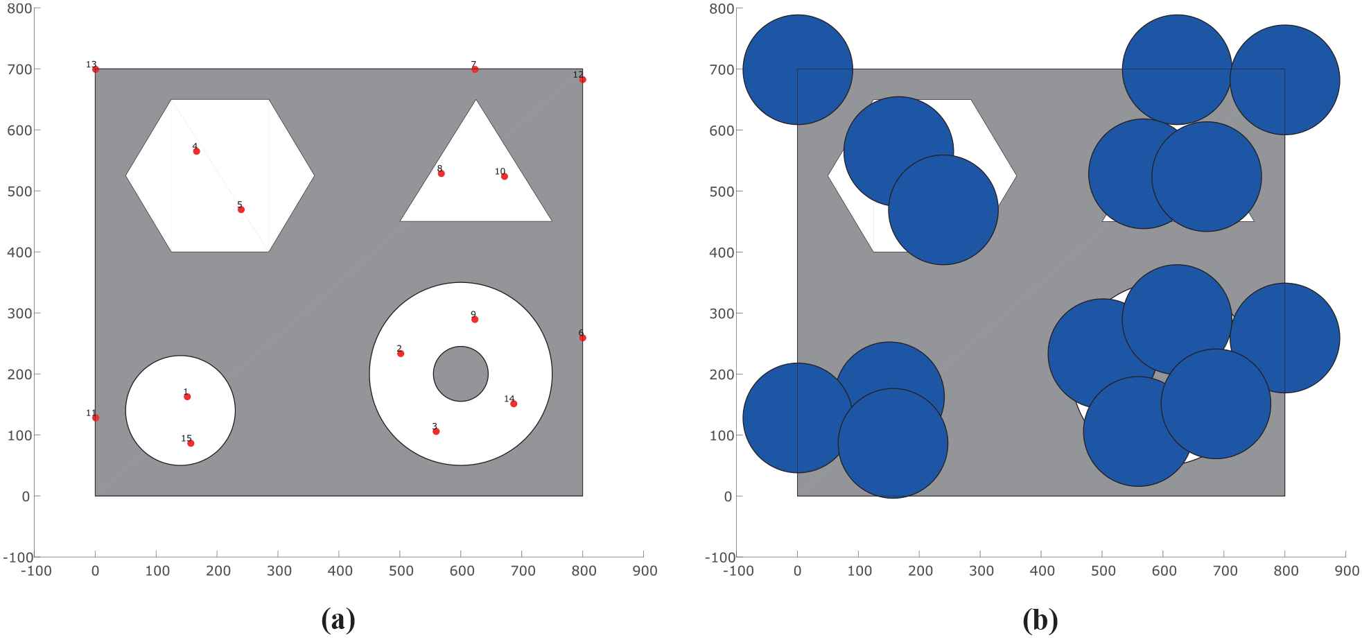
Initial configuration of positions for a set of 15 sensor nodes deployed to cover a set of disjointed regions of interest (ROIs) within an experimental environment of area size A = 800 × 700: (a) sensor nodes locations and (b) area covered by the sensing devices on their initial locations.
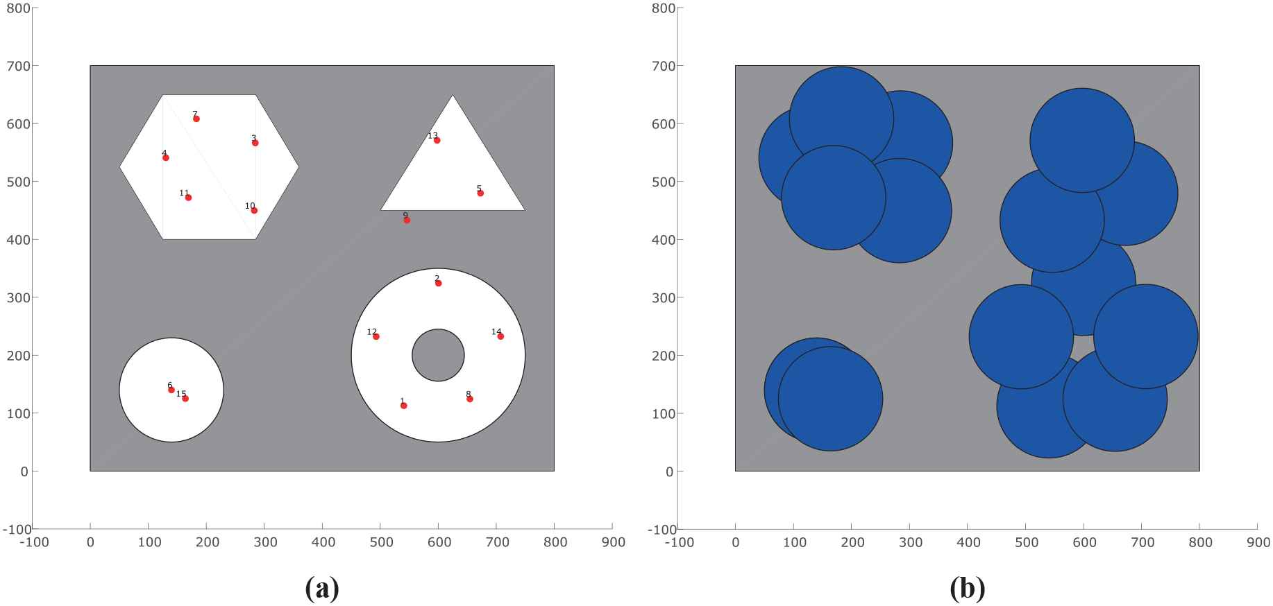
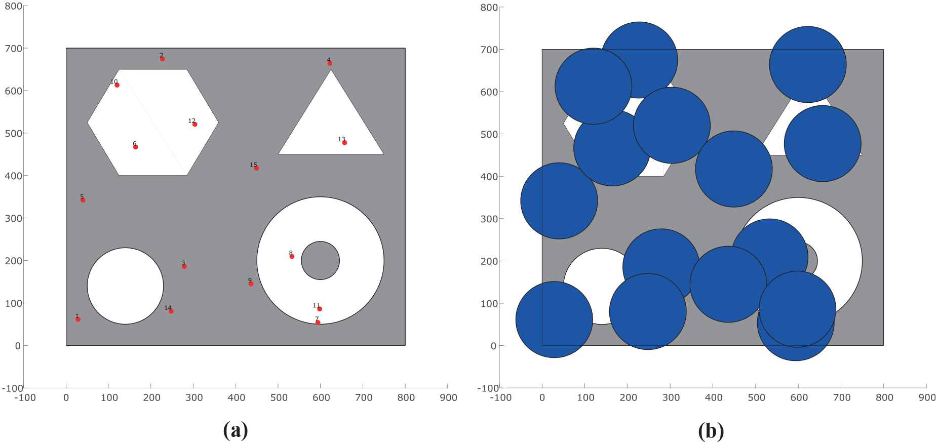
Positions configuration for a set of 15 sensor nodes deployed to cover a set of disjointed regions of interest (ROIs) within an experimental environment of area size A = 800 × 700, obtained by applying the real-coded Social Spider Optimization (R-SSO) approach: (a) sensor nodes locations, and (b) area covered by the deployed sensing devices.
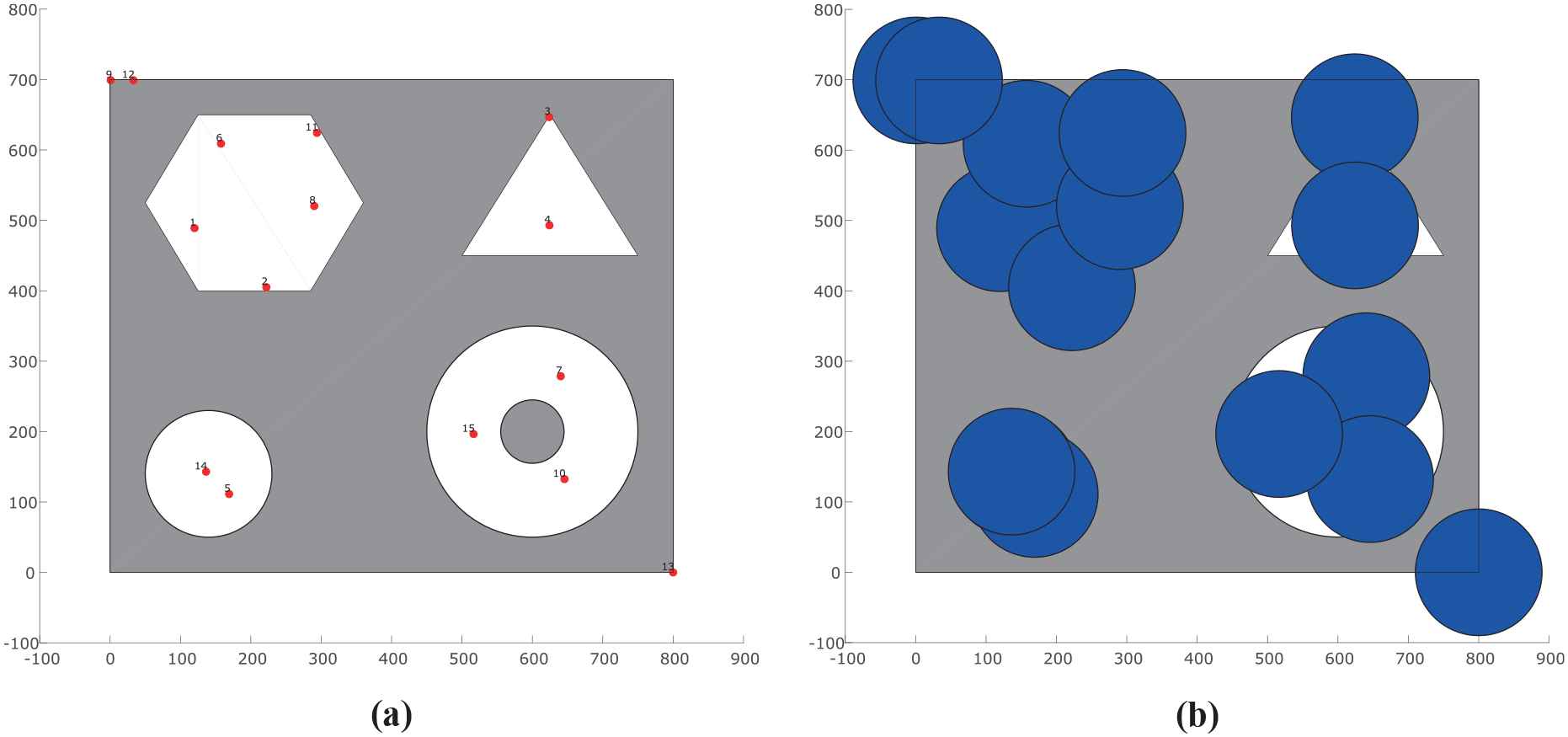
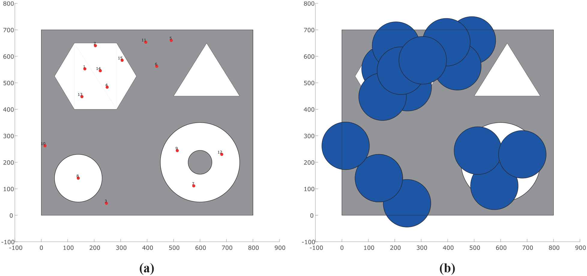
Positions configuration for a set of 15 sensor nodes deployed to cover a set of disjointed regions of interest (ROIs) within an experimental environment of area size A = 800 × 700, obtained by applying the Moth-flame Optimization (MFO) approach: (a) sensor nodes locations and (b) area covered by the deployed sensing devices.
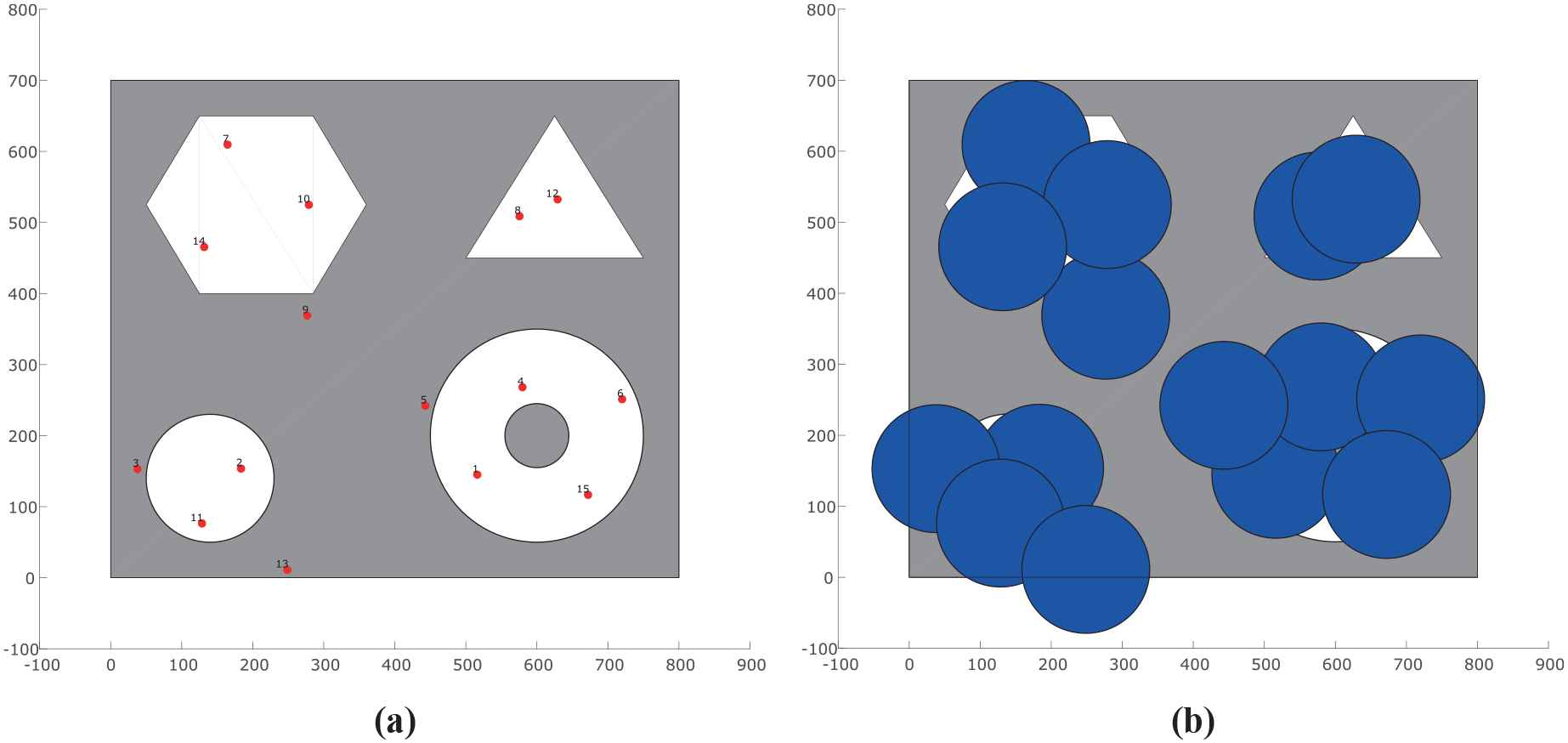
Positions configuration for a set of 15 sensor nodes deployed to cover a set of disjointed regions of interest (ROIs) within an experimental environment of area size A = 800 × 700, obtained by applying the Firefly Algorithm (FA) approach: (a) sensor nodes locations and (b) area covered by the deployed sensing devices.
Positions configuration for a set of 15 sensor nodes deployed to cover a set of disjointed regions of interest (ROIs) within an experimental environment of area size A = 800 × 700, obtained by applying the Particle Swarm Optimization (PSO) approach: (a) sensor nodes locations and (b) area covered by the deployed sensing devices.
Positions configuration for a set of 15 sensor nodes deployed to cover a set of disjointed regions of interest (ROIs) within an experimental environment of area size A = 800 × 700, obtained by applying the Crow Search Algorithm (CSA) approach: (a) sensor nodes locations and (b) area covered by the deployed sensing devices.

Positions configuration for a set of 15 sensor nodes deployed to cover a set of disjointed regions of interest (ROIs) within an experimental environment of area size A = 800 × 700, obtained by applying the Artificial Bee Colony (ABC) approach: (a) sensor nodes locations and (b) area covered by the deployed sensing devices.
Positions configuration for a set of 15 sensor nodes deployed to cover a set of disjointed regions of interest (ROIs) within an experimental environment of area size A = 800 × 700, obtained by applying the Whale Optimization Algorithm (WOA) approach: (a) sensor nodes locations and (b) area covered by the deployed sensing devices.

Positions configuration for a set of 15 sensor nodes deployed to cover a set of disjointed regions of interest (ROIs) within an experimental environment of area size A = 800 × 700, obtained by applying the Grey Wolf Optimizer (GWO) approach: (a) sensor nodes locations and (b) area covered by the deployed sensing devices.
6. CONCLUSIONS
In this paper, a real-coded sensor deployment approach based on the SSO algorithm has been proposed to solve the problem of OSD in WSNs. Different to most of the methods currently reported on the literature, which only consider a set of discrete-coded locations as candidate positions to deploy sensor nodes, our proposed method is able to explore any spatial location within a given ROI. Under our proposed approach, two technical challenges commonly seen within the problem of OSD are handled: on first instance, by considering real candidate locations instead of a set of finite discrete locations our proposed method has the flexibility to explore potentially better solutions to the sensor deployment problem, while also increasing its performance when placement restrictions are introduced; on second place, since the actual covered area is considered for calculating the rate coverage of a given sensor arrangement configuration, the uncertainty of the model is reduced, as this approach provides a better insight on the actual amount of the ROI that is being monitored by the deployed sensor network.
In order to evaluate the performance of our proposed method, a collection of comparative experiments which evaluate the performance of our proposed method against other similar approaches have been conducted. Our experimental results are divided three separated stages: for our first set of experiments, we have compared the performance of our R-SSO-based OSD approach against that of the D-SSO method previously proposed in [19]; for the second stage, we have compared the performance of our R-SSO approach against other metaheuristics-based methods adapted to work in terms of real-coded OSD, which include optimization schemes such as the MFO algorithm [20], FA [21], PSO [22], ABC [23], WOA [24], CSA [25], and GWO [26]. Finally, for our third and final set of experiments, we have compared the performance of R-SSO, MFO, FA, PSO, CSA, BA, WOA, and GWO with regard to a special case of OSD. As in the previous two sets of experiments, this study involved the OSD of a WSN, aimed cover several specific disjointed regions of different shape and size within the proposed experimental environment, an experiment not commonly seen on the literature.
In all of the performed experiments, the proposed R-SSO OSD approach has demonstrated to have the best performance when compared to all other of the compared methods. The remarkable performance produced by our proposed scheme is related to two important characteristics of the R-SSO algorithm: 1. its task division scheme, which allows the SSO population to be divided in two subpopulations with different functions and 2. the specialized operators applied by male and female spiders, which allows them to experiment different behaviors as the search process goes on. In general, these properties allow the SSO algorithm to manifest a better tradeoff between the exploration and exploitation of solutions, thus enhancing the probability to find more competent solutions.
CONFLICT OF INTEREST
The authors declare that there are no conflict of interest implicted in this work.
AUTHORS' CONTRIBUTIONS
All authors are credited for their contribution on the writing and revisions of the submitted manuscript.
All of the experiments reported in this paper were designed and performed by Oscar Maciel-Castillo and Bernardo a Morales-Castañeda
The data and results presented on this work were analyzed and validated Fernando Fausto and Erik Cuevas.
ACKNOWLEDGMENTS
The completion of this work wouldn't have been possible without the colaboration of Dr. Oscar Maciel-Castillo and Dr. Bernardo Morales-Castañeda, who designed and performed all of the experiments reported in this manuscript. We also thanks Dr. Erik Cuevas for their valuable assistance and observations during the development of this work.
REFERENCES
Cite this article
TY  - JOUR
AU  - Fernando Fausto
AU  - Erik Cuevas
AU  - Oscar Maciel-Castillo
AU  - Bernardo Morales-Castañeda
PY  - 2019
DA  - 2019/06/06
TI  - A Real-Coded Optimal Sensor Deployment Scheme for Wireless Sensor Networks Based on the Social Spider Optimization Algorithm
JO  - International Journal of Computational Intelligence Systems
SP  - 676
EP  - 696
VL  - 12
IS  - 2
SN  - 1875-6883
UR  - https://doi.org/10.2991/ijcis.d.190614.001
DO  - 10.2991/ijcis.d.190614.001
ID  - Fausto2019
ER  -