
A Fuzzy-Random Extension of the Lee–Carter Mortality Prediction Model
- DOI
- 10.2991/ijcis.d.190626.001How to use a DOI?
- Keywords
- Lee–Carter model; Fuzzy numbers; Fuzzy regression; Fuzzy-random modeling
- Abstract
The Lee–Carter model is a useful dynamic stochastic model to represent the evolution of central mortality rates throughout time. This model only considers the uncertainty about the coefficient related to the mortality trend over time but not to the age-dependent coefficients. This paper proposes a fuzzy-random extension of the Lee–Carter model that allows quantifying the uncertainty of both kinds of parameters. As it is commonplace in actuarial literature, the variability of the time-dependent index is modeled as an ARIMA time series. Likewise, the uncertainty of the age-dependent coefficients is also quantified, but by using triangular fuzzy numbers. The consideration of this last hypothesis requires developing and solving a fuzzy regression model. Once the fuzzy-random extension has been introduced, it is also shown how to obtain some variables linked with central mortality rates such as death probabilities or life expectancies by using fuzzy numbers arithmetic. It is simultaneously shown the applicability of our developments with data of Spanish male population in the period 1970–2012. Finally we make a comparative assessment of our method with alternative Lee–Carter model estimates on 16 Western Europe populations.
- Copyright
- © 2019 The Authors. Published by Atlantis Press SARL.
- Open Access
- This is an open access article distributed under the CC BY-NC 4.0 license (http://creativecommons.org/licenses/by-nc/4.0/).
1. INTRODUCTION
Classical actuarial methods graduate mortality by only taking into account the age of persons without calendar year considerations. Due to the progressive increase of life expectancy in all developed countries, this kind of methods systematically overestimate the mortality rates and, as a consequence, may increase the longevity risk when pricing life annuities.
In the last decades of the 20th century, several papers developed dynamic stochastic approaches for the evolution of mortality rates throughout calendar time and, so, projecting mortality to the future with these models became more accurate. In this way, the method in [1], that we will name Lee–Carter (LC), is one of the most extended methodologies. The LC model proposed adjusting a linear function to the logarithm of central mortality rates of each year and age,
There are two main reasons why the LC model boasts great acceptance. On the one hand, it has been applied in many countries with good results [2–10]. Likewise, the LC method is relatively easy to compute in its seminal version, either by using the singular value decomposition (SVD) method or with the approximation to the SVD solution suggested in [1].
Several papers proposed technical extensions to the original LC model as [3,5–7,11–13]. All these extensions have two common features. Firstly, more completeness and sophistication of the model suppose more computational effort. Secondly, all of them consider that the age-specific historical influences not captured by the model are due to a stochastic error-term, as the LC model does. However, stochastic variability may not be the unique source of uncertainty since it can also come from fuzziness (e.g., due to incomplete or imprecise information) and, consequently, it can be modeled with Fuzzy Sets Theory tools. In this way, [14] developed two alternative fuzzy formulations of the LC model. The first model considers that all the parameters are fuzzy numbers (FNs) and arithmetical operations are carried out by means of the weakest t-norm. This first approach was object of several refinements in [15,16]. In the second approach, the centers and spreads of the FNs that estimate the parameters of the LC model are supposed to be random variables (RVs) and are estimated with Bayesian methods. The comparison between the fuzzy and the fuzzy-stochastic models seems to show very similar results, but the second model requires much more computational effort.
Mixing fuzziness and randomness in actuarial modeling is not new. [17] described fuzzy RVs with actuarial applications in view and [18] developed a non-life individual risk model where the number of claims follows a Poisson process and their amount is estimated with a triangular fuzzy number (TFN). In a life insurance context, [19,20] used fuzzy RVs for the valuation of life contingencies.
This paper also blends fuzziness and randomness and proposes a fuzzy-random approach of the LC model which is conceptually different to those developed in [14]. We consider that the behavior of the independent variable
In order to adjust the fuzzy coefficients of the logarithm of
The rest of the paper is organized as follows: We firstly make a brief review of the LC model. Then, we describe some concepts of FNs and FR that will be necessary to develop our work. Section 4 features our fuzzy-random extension to the LC model, exposes how to project future mortality from this formulation, and shows an empirical application for Spanish male population, evaluating both the capability of the model to adjust central mortality rates to sample data and to predict out-of-sample data. In the fifth section, we show how some mortality tables variables can be obtained from the results of previous sections. Subsequently, focused on life expectancies of Spanish male population, we test the capability of our model to predict future values. Section 6 includes a complete comparison of the predictive performance of the proposed method with both the basic LC method in [1] and the fuzzy extension by Koissi and Shapiro in [14]. This comparison shows the advantages of our fuzzy-random extension of the LC model. We finish the work by pointing out the main conclusions and suggesting possible extensions.
2. OVERVIEW OF THE LEE–CARTER MODEL
Lee and Carter in [1] proposed modeling the logarithm of the central death rate for each specific age and each year with a linear function. In such a way, if
Notice that whereas the parameters
The model Equation (1) cannot be fitted by ordinary regression techniques because on its right side there are two parameters to be estimated but
And finally, each
Once the parameters of the model have been fitted, for
3. FNS AND FR
3.1. FNs and Their Arithmetic
This paper quantifies uncertain quantities as a common type of FN, TFNs, that will be symbolized as
The expected interval of a FN
Let f be a continuous real-valued function of n-real variables
The result of evaluating nonlinear functions with TFNs is not a TFN. In this way, [24] proposed a TFN approximation for any real-valued function, derivable and increasing (decreasing) respect to the first (last) m (n − m) variables, built up from the first-order Taylor polynomial expansion from the 1-cut to any α-cut. It can be demonstrated that in Equation (5)
Arithmetic operations between real numbers can be extended to FNs by using the appropriate real-valued function. Since this work uses TFNs, when this function is linear the result of the arithmetic operation will also be a TFN. Otherwise, the result will be approximated by using Equation (6). So, it is obtained:
Addition:
Scalar multiplication:
Product of two positive TFNs (i.e., their supports are contained within
Division of two positive TFNs:
Exponential function:
Logarithmic function:
3.2. FR Model with Asymmetric Coefficients
This paper uses the FR model of [21] that combines the least squares method with the minimum fuzziness principle in [22]. This type of FR method has been used in financial and actuarial applications like fitting options volatility smile [25,26] or calculating claim reserves [27]. In the actuarial field, a wide survey of FR models can be found in [28].
Let us suppose that for the
The final objective is obtaining the estimates of
Step 1. By taking the centers of the dependent variable,
Step 2. We fit the spreads of parameters applying the minimum fuzziness criterion in [22]. So, spread estimates must minimize the uncertainty of the estimated outputs and simultaneously these estimated outputs have to contain the real observations, with a membership level of at least
Considering, as in [22], that
And accomplish the constraints
[29] proposed a rule to choose
If we name as
Thus, the credibility for the entire sample
Therefore, the process that we follow to fit the fuzzy coefficients consists in implementing Step 2 for
4. FUZZY-RANDOM APPROACH OF THE LC MODEL
4.1. Fuzzy-Random Fitting of the LC Model
Our fuzzy-random approach of the LC model considers two different sources of uncertainty:
It is supposed that historical influences of each specific age are due to fuzziness in the model structure. As a consequence, both, the coefficient that describes the average age-specific pattern of mortality and the coefficient which reflects the variation in the central death across time, turn into FNs and so
The mortality index
Under these assumptions, once the average pattern of mortality,
In order to fit the estimates
Step 1. By taking the centers of
Step 2. We have to calculate the values
Let us remark that the constraints
Step 3. We obtain the optimal value
By using
4.2. Forecasting with the Fuzzy-Random LC Model
To forecast future central mortality rates and related variables, it is necessary projecting the values of the index
[31] developed a framework for predictions that mixes conventional regression and fuzzy parameters. Following those developments, the predicted values of kt,
We can use three different estimates for kt,
If we use the mathematical expectation,
that can be calculated with Equations. (10a–10d). So, the central rate of mortality obtained fromwhich can be approximated by a TFN using Equation (11).If we estimate kt by its
- –
If
- –
If
And it can be implemented with Equations (10a–10d). The central rate of mortality obtained from
and this FN can also be approximated with Equation (11).Of course, with this procedure, we maintain the fuzzy uncertainty of
- –
If we take for kt its probabilistic
If
If
In both cases, we have to apply Equations (13a–13b).
To calculate the bounds of the fuzzy-probabilistic confidence interval
Let us remark that [1] did not take into account the uncertainty of
4.3. An Empirical Application of the Fuzzy-Random LC Model: The Case of Spanish Male Population
We apply our extension of the LC model to Spanish male population within the period 1970–2000 and we test its out-of-sample performance during 2001–2012. Central mortality rates have been collected from the “Human Mortality Database,” [32] (http://www.mortality.org). Ages are grouped in 5-year intervals, except for ages less than 1 year, for ages from 1 to 5 years, and for ages greater or equal to 110 years. The values of the estimates
| Age | Center | Left Spread | Right Spread | Center | Left Spread | Right Spread |
|---|---|---|---|---|---|---|
| [0, 1) | −4.49273 | 0.30688 | 0.25300 | 0.17351 | 0.00000 | 0.00000 |
| [1, 5) | −7.48194 | 0.20455 | 0.18860 | 0.12731 | 0.00000 | 0.00000 |
| [5, 10) | −8.10376 | 0.21022 | 0.22686 | 0.11147 | 0.00000 | 0.00000 |
| [10, 15) | −8.11329 | 0.12371 | 0.11770 | 0.08472 | 0.00000 | 0.01665 |
| [15, 19) | −7.17041 | 0.12666 | 0.21927 | 0.03932 | 0.00000 | 0.02229 |
| [20, 24) | −6.77416 | 0.12234 | 0.33523 | 0.02428 | 0.00000 | 0.02060 |
| [25, 29) | −6.64539 | 0.19804 | 0.43116 | 0.00113 | 0.00000 | 0.00113 |
| [30, 34) | −6.47171 | 0.30079 | 0.29775 | −0.01338 | 0.01338 | 0.00000 |
| [35, 39) | −6.25015 | 0.17167 | 0.12575 | 0.00356 | 0.00356 | 0.00000 |
| [40, 44) | −5.89617 | 0.07598 | 0.04676 | 0.02483 | 0.00243 | 0.00000 |
| [45, 49) | −5.45921 | 0.06226 | 0.02487 | 0.03075 | 0.00000 | 0.00520 |
| [50, 54) | −5.00591 | 0.05166 | 0.05161 | 0.03864 | 0.00000 | 0.00000 |
| [55, 59) | −4.55867 | 0.06395 | 0.05231 | 0.04121 | 0.00000 | 0.00087 |
| [60, 64) | −4.10372 | 0.08045 | 0.05451 | 0.04445 | 0.00000 | 0.00000 |
| [65, 69) | −3.64283 | 0.07091 | 0.04687 | 0.04724 | 0.00000 | 0.00523 |
| [70, 74) | −3.15519 | 0.07888 | 0.05236 | 0.05065 | 0.00030 | 0.00000 |
| [75, 79) | −2.66456 | 0.09569 | 0.05943 | 0.04685 | 0.00210 | 0.00000 |
| [80, 84) | −2.18259 | 0.07938 | 0.05492 | 0.04257 | 0.00203 | 0.00001 |
| [85, 89) | −1.72857 | 0.06846 | 0.04214 | 0.03342 | 0.00580 | 0.00000 |
| [90, 94) | −1.32104 | 0.06281 | 0.04782 | 0.02257 | 0.00465 | 0.00028 |
| [95, 99) | −0.97328 | 0.04833 | 0.02706 | 0.01436 | 0.00810 | 0.00692 |
| [100, 104) | −0.68435 | 0.05068 | 0.02508 | 0.00759 | 0.00636 | 0.00759 |
| [105, 109) | −0.46013 | 0.04953 | 0.03142 | 0.00277 | 0.00000 | 0.00277 |
| [110, ∞) | −0.31708 | 0.04852 | 0.03221 | 0.00017 | 0.00000 | 0.00017 |
Parameters
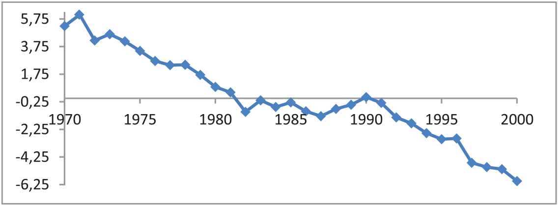
Evolution of kt for Spanish male population in the period 1970–2000.
The unit root test [33] on
In Table 2, Ljung and Box Q-statistic suggests that a pure random walk for the first difference is acceptable. So, we model kt as
| Lag | Autocorrelation | Partial Autocorrelation | Q-Statistic | p-Value |
|---|---|---|---|---|
| 1 | −0.305 | −0.305 | 30.004 | 0.120 |
| 2 | 0.145 | 0.005 | 38.019 | 0.149 |
| 3 | −0.01 | 0.054 | 38.053 | 0.283 |
| 4 | −0.101 | −0.109 | 41.836 | 0.382 |
| 5 | 0.174 | 0.123 | 53.422 | 0.376 |
| 6 | −0.023 | 0.092 | 53.638 | 0.498 |
| 7 | −0.002 | −0.004 | 53.927 | 0.612 |
| 8 | −0.112 | −0.174 | 59.353 | 0.654 |
| 9 | −0.333 | −0.437 | 11.001 | 0.276 |
| 10 | 0.014 | −0.055 | 12.450 | 0.256 |
| 11 | 0.22 | −0.152 | 14.886 | 0.188 |
| 12 | 0.11 | −0.023 | 15.530 | 0.215 |
Autocorrelation statistics for the time series
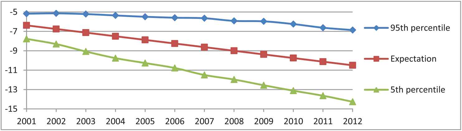
Estimation of the evolution of kt for Spanish male population in the period 2001–2012.
We now check the capability of our extension of the LC model to fit the central rate of mortality,
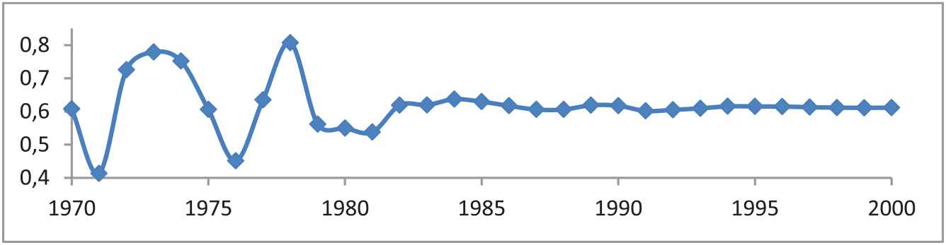
Values of

Values of
Figure 3 shows that the mean grade of membership until the middle of the 80s oscillates, depending on the year, between 0.4 and 0.8. Subsequently,
Table 3 shows the TFN predictions for the central mortality rates of year 2010 that come from
| Age | Center | Left Spread | Right Spread | Center | Left Spread | Right Spread | Center | Left Spread | Right Spread |
|---|---|---|---|---|---|---|---|---|---|
| [0, 1) | 0.00206 | 0.00063 | 0.00052 | 0.00115 | 0.00035 | 0.00029 | 0.00379 | 0.00116 | 0.00096 |
| [1, 5) | 0.00016 | 0.00003 | 0.00003 | 0.00011 | 0.00002 | 0.00002 | 0.00025 | 0.00005 | 0.00005 |
| [5, 10) | 0.00010 | 0.00002 | 0.00002 | 0.00007 | 0.00001 | 0.00002 | 0.00015 | 0.00003 | 0.00003 |
| [10, 15) | 0.00013 | 0.00004 | 0.00002 | 0.00010 | 0.00003 | 0.00001 | 0.00018 | 0.00004 | 0.00002 |
| [15, 19) | 0.00052 | 0.00018 | 0.00011 | 0.00046 | 0.00019 | 0.00010 | 0.00060 | 0.00016 | 0.00013 |
| [20, 24) | 0.00090 | 0.00029 | 0.00030 | 0.00083 | 0.00033 | 0.00028 | 0.00098 | 0.00025 | 0.00033 |
| [25, 29) | 0.00129 | 0.00037 | 0.00055 | 0.00128 | 0.00038 | 0.00055 | 0.00129 | 0.00037 | 0.00056 |
| [30, 34) | 0.00176 | 0.00053 | 0.00087 | 0.00168 | 0.00051 | 0.00075 | 0.00184 | 0.00055 | 0.00100 |
| [35, 39) | 0.00186 | 0.00032 | 0.00047 | 0.00184 | 0.00032 | 0.00049 | 0.00189 | 0.00032 | 0.00045 |
| [40, 44) | 0.00216 | 0.00016 | 0.00015 | 0.00199 | 0.00015 | 0.00016 | 0.00235 | 0.00018 | 0.00015 |
| [45, 49) | 0.00315 | 0.00036 | 0.00008 | 0.00284 | 0.00037 | 0.00007 | 0.00351 | 0.00033 | 0.00009 |
| [50, 54) | 0.00460 | 0.00024 | 0.00024 | 0.00403 | 0.00021 | 0.00021 | 0.00526 | 0.00027 | 0.00027 |
| [55, 59) | 0.00701 | 0.00051 | 0.00037 | 0.00610 | 0.00046 | 0.00032 | 0.00810 | 0.00056 | 0.00042 |
| [60, 64) | 0.01070 | 0.00086 | 0.00058 | 0.00922 | 0.00074 | 0.00050 | 0.01251 | 0.00101 | 0.00068 |
| [65, 69) | 0.01651 | 0.00201 | 0.00077 | 0.01409 | 0.00197 | 0.00066 | 0.01949 | 0.00202 | 0.00091 |
| [70, 74) | 0.02602 | 0.00205 | 0.00144 | 0.02194 | 0.00173 | 0.00124 | 0.03107 | 0.00245 | 0.00169 |
| [75, 79) | 0.04410 | 0.00422 | 0.00352 | 0.03766 | 0.00360 | 0.00327 | 0.05196 | 0.00497 | 0.00377 |
| [80, 84) | 0.07445 | 0.00592 | 0.00556 | 0.06450 | 0.00513 | 0.00526 | 0.08642 | 0.00687 | 0.00584 |
| [85, 89) | 0.12816 | 0.00877 | 0.01264 | 0.11452 | 0.00784 | 0.01353 | 0.14409 | 0.00986 | 0.01129 |
| [90, 94) | 0.21414 | 0.01404 | 0.01994 | 0.19846 | 0.01321 | 0.02159 | 0.23176 | 0.01497 | 0.01781 |
| [95, 99) | 0.32848 | 0.03803 | 0.03485 | 0.31297 | 0.04353 | 0.04175 | 0.34543 | 0.03162 | 0.02684 |
| [100, 104) | 0.46845 | 0.05871 | 0.04225 | 0.45663 | 0.06889 | 0.05097 | 0.48107 | 0.04750 | 0.03266 |
| [105, 109) | 0.61439 | 0.05071 | 0.03279 | 0.60868 | 0.05592 | 0.03249 | 0.62038 | 0.04519 | 0.03311 |
| [110, ∞) | 0.72704 | 0.03900 | 0.04508 | 0.72661 | 0.03941 | 0.04506 | 0.72748 | 0.03858 | 0.04511 |
TFN, triangular fuzzy number.
TFN approximations of the estimates of
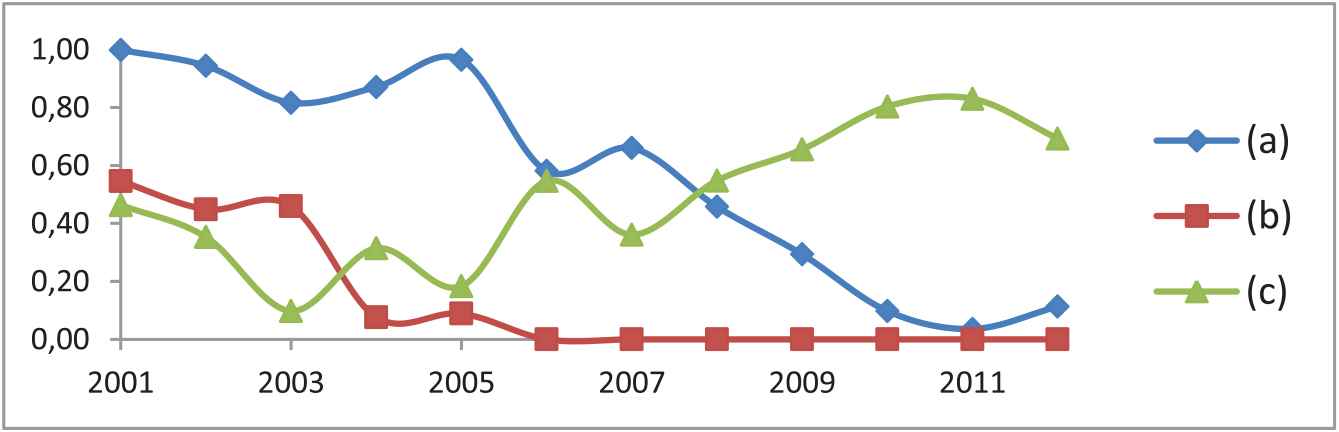
Figure 5 depicts the membership level of true observed values of
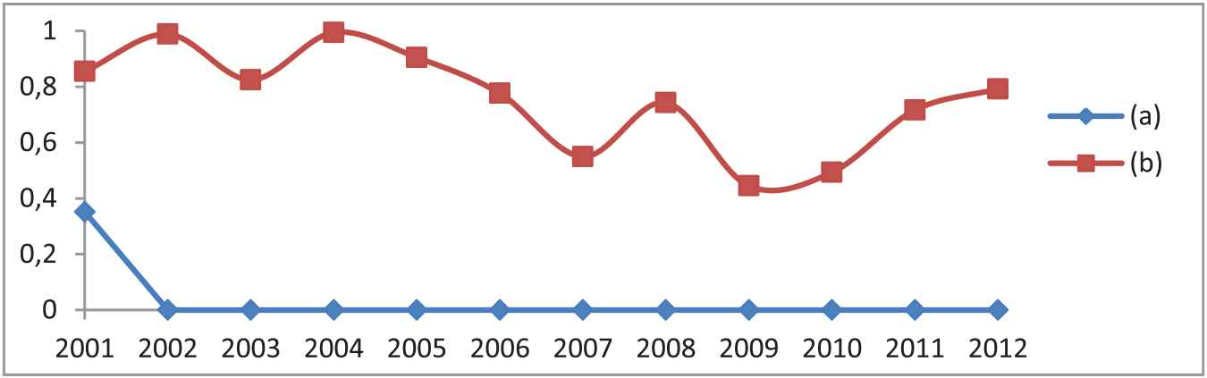
Membership levels
Note: (a) stands for
| Year | W | Median | Mean | Year | W | Median | Mean |
|---|---|---|---|---|---|---|---|
| 2001 | 92* | 0.602 | 0.656 | 2007 | 93 | 0.414 | 0.381 |
| 2002 | 141 | 0.488 | 0.643 | 2008 | 141 | 0.438 | 0.256 |
| 2003 | 77** | 0.181 | 0.439 | 2009 | 59** | 0.534 | 0.246 |
| 2004 | 140 | 0.454 | 0.431 | 2010 | 122 | 0.462 | 0.233 |
| 2005 | 117 | 0.165 | 0.337 | 2011 | 67*** | 0.521 | 0.255 |
| 2006 | 61*** | 0.528 | 0.320 | 2012 | 62*** | 0.202 | 0.182 |
Notes: (1)
Assessment of the capability prediction of
5. FORECASTING LIFE EXPECTANCY WITH THE FUZZY-RANDOM LC MODEL
5.1. Calculating Life Expectancy from Fuzzy Estimates of Central Mortality Rates
We now compute probabilities of death or survival and life expectancies after calculating estimates of central mortality rates. Let us denote the width of the age group as
To obtain the probability that a person in the age group
It may be useful to obtain a triangular approximation for
In order to obtain the support of
To determine the probability that a person in the age group
From Equations (15a–15c),
The life expectancy of a person in the age group
Since
| Year | Center | Left Spread | Right Spread | Center | Left Spread | Right Spread | Center | Left Spread | Right Spread |
|---|---|---|---|---|---|---|---|---|---|
| 2001 | 76.31 | 1.18 | 1.28 | 75.73 | 1.17 | 1.28 | 76.96 | 1.20 | 1.28 |
| 2002 | 76.49 | 1.19 | 1.28 | 75.72 | 1.17 | 1.28 | 77.20 | 1.21 | 1.29 |
| 2003 | 76.66 | 1.19 | 1.28 | 75.75 | 1.17 | 1.28 | 77.54 | 1.22 | 1.29 |
| 2004 | 76.84 | 1.20 | 1.28 | 75.82 | 1.18 | 1.28 | 77.85 | 1.23 | 1.30 |
| 2005 | 77.01 | 1.20 | 1.29 | 75.89 | 1.18 | 1.28 | 78.07 | 1.24 | 1.30 |
| 2006 | 77.18 | 1.21 | 1.29 | 75.94 | 1.18 | 1.28 | 78.29 | 1.25 | 1.30 |
| 2007 | 77.35 | 1.21 | 1.29 | 75.94 | 1.18 | 1.28 | 78.60 | 1.27 | 1.31 |
| 2008 | 77.52 | 1.22 | 1.29 | 75.97 | 1.18 | 1.28 | 78.80 | 1.28 | 1.31 |
| 2009 | 77.69 | 1.23 | 1.29 | 76.10 | 1.18 | 1.28 | 79.05 | 1.29 | 1.32 |
| 2010 | 77.85 | 1.23 | 1.30 | 76.13 | 1.18 | 1.28 | 79.28 | 1.31 | 1.32 |
| 2011 | 78.02 | 1.24 | 1.30 | 76.26 | 1.18 | 1.28 | 79.50 | 1.32 | 1.33 |
| 2012 | 78.19 | 1.25 | 1.30 | 76.56 | 1.19 | 1.28 | 79.75 | 1.34 | 1.33 |
TFN, triangular fuzzy number.
TFN approximation of the estimates of
By evaluating Equation (17) with
A TFN approximation of
Of course, if in Equations (18a–18c) we take as a prediction of the index kt its mathematical expectation,
If the prediction of the mortality trend comes from its probabilistic confidence interval,
| Year | Center | Left Spread | Right Spread | Center | Left Spread | Right Spread | Center | Left Spread | Right Spread |
|---|---|---|---|---|---|---|---|---|---|
| 2001 | 17.06 | 0.48 | 0.64 | 16.67 | 0.46 | 0.63 | 17.51 | 0.51 | 0.65 |
| 2002 | 17.18 | 0.49 | 0.64 | 16.66 | 0.46 | 0.63 | 17.68 | 0.52 | 0.65 |
| 2003 | 17.30 | 0.49 | 0.64 | 16.68 | 0.46 | 0.63 | 17.92 | 0.53 | 0.66 |
| 2004 | 17.42 | 0.50 | 0.65 | 16.73 | 0.46 | 0.63 | 18.15 | 0.55 | 0.66 |
| 2005 | 17.54 | 0.51 | 0.65 | 16.78 | 0.46 | 0.63 | 18.31 | 0.56 | 0.67 |
| 2006 | 17.67 | 0.52 | 0.65 | 16.82 | 0.47 | 0.63 | 18.47 | 0.57 | 0.67 |
| 2007 | 17.79 | 0.52 | 0.66 | 16.82 | 0.47 | 0.63 | 18.70 | 0.58 | 0.67 |
| 2008 | 17.91 | 0.53 | 0.66 | 16.83 | 0.47 | 0.63 | 18.85 | 0.59 | 0.68 |
| 2009 | 18.03 | 0.54 | 0.66 | 16.92 | 0.47 | 0.63 | 19.04 | 0.61 | 0.68 |
| 2010 | 18.15 | 0.55 | 0.66 | 16.94 | 0.47 | 0.64 | 19.21 | 0.62 | 0.68 |
| 2011 | 18.27 | 0.55 | 0.67 | 17.03 | 0.48 | 0.64 | 19.38 | 0.63 | 0.69 |
| 2012 | 18.40 | 0.56 | 0.67 | 17.24 | 0.49 | 0.64 | 19.57 | 0.64 | 0.69 |
TFN, triangular fuzzy number.
TFN approximation of the estimates of
5.2. Predicting Life Expectancies of Spanish Male Population in 2001–2012
Tables 5 and 6 show the estimates for the mean value and the 90% confidence fuzzy-probabilistic interval of the life expectancy for the age groups [0, 1) and [65, 69) during the period 2001–2012. These ages are significantly important because they are considered in order to quantify life expectancy at birth and at retirement, respectively. If only the centers of the fuzzy life expectancies are considered, predictions that come from the basic LC method are found. So, for example, the point estimate for
Figures 6 and 7 represent the membership level of true observed values for life expectancies,
Membership levels
Note: (a) stands for
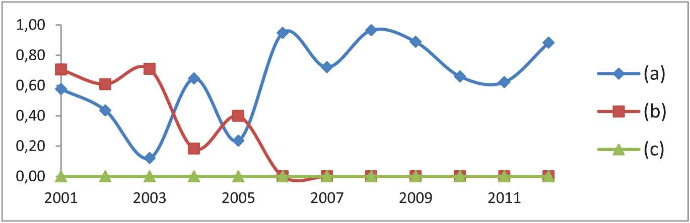
Membership levels
Note: (a) stands for
| Capability Prediction of |
|||||||
|---|---|---|---|---|---|---|---|
| Year | W | Median | Mean | Year | W | Median | Mean |
| 2001 | 92* | 0.602 | 0.718 | 2007 | 93 | 0.414 | 0.589 |
| 2002 | 141 | 0.488 | 0.656 | 2008 | 141 | 0.438 | 0.586 |
| 2003 | 77** | 0.181 | 0.338 | 2009 | 59*** | 0.534 | 0.555 |
| 2004 | 140 | 0.454 | 0.653 | 2010 | 122 | 0.462 | 0.445 |
| 2005 | 117 | 0.165 | 0.440 | 2011 | 67*** | 0.521 | 0.443 |
| 2006 | 61*** | 0.528 | 0.699 | 2012 | 62*** | 0.202 | 0.409 |
| Capability Prediction of |
|||||||
| Median | Mean | W | |||||
| 0.628 | 0.567 | 37 | |||||
| 0.655 | 0.609 | 19 | |||||
Notes: (1) Each year has 24 predictions on life expectancies, one per age group. (2) Each age group has 12 predictions available, one for each assessed year. (3)
Assessment of the capability prediction of
Due to the interest in actuarial analyses in life expectancy both at birth and at retirement, we test the quality of the prediction by
6. EMPIRICAL ASSESSMENT OF THE FUZZY-RANDOM LC MODEL IN EIGHT WESTERN EUROPEAN COUNTRIES1
6.1. Methodological Considerations
In this section we make a comparative assessment on the prediction capability of our proposed fuzzy-random extension of the LC model (FRLC) with both the basic LC (BLC) in [1] and the pure fuzzy LC version by Koissi and Shapiro in [14], (FKSLC). Let us remark that BLC only considers random uncertainty of coefficients
To carry out the analysis, we use central mortality rates collected separately for men and women in eight Western Europe countries (i.e., we use 16 databases) from [32] (http://www.mortality.org). As we made in Sections 4 and 5 for the case of Spanish male population, we fit the model parameters by using central mortality rates in the period 1970–2000 and we test models out-of-sample performance during 2001–2012. Ages are again grouped in 5-year intervals, except for ages lower than 1 year, for ages from 1 to 5 years, and for ages greater or equal to 110 years.
We assess two aspects regarding the fitting quality of the models:
Item 1. We measure and compare models' performance to make point predictions on central mortality rates and life expectancies. This is made by using the conventional error measures: root mean squared error (RMSE), normalized mean squared error (NMSE), and mean absolut error (MAE). We consider these point predictions: the expectation for BLC, the core of the fuzzy expectation for FRLC and, finally, the core of the fuzzy prediction for FKSLC. Notice that point predictions by BLC and FRLC are the same by definition. So, in fact, we are making a comparison of a couple of predictive methods: BLC/FRLC versus FKSLC. Following [36], this pairwise comparison between techniques is made with both a sign test (Wins/Losses) and a Wilcoxon rank test.
Item 2. We evaluate the capability of BLC, FRLC, and FKSLC to predict future values of
In this regard, let us make the following remarks:
BLC only considers random uncertainty of
FRLC estimates the lower and upper bounds of the
FKSLC directly predicts mortality variables as FNs. The expected interval of the FN obtained from this method is taken as its confidence interval.
The analysis of both questions is developed in two levels:
In each population, we independently assess the predictive capability of each method. For a given population we must predict 24 variables for each of the 12 years that testing period 2001–2012 comprises. In each year we find the mean value of the accuracy measures and so, for each population, we have 12 available mean values of accuracy (one per year). The results that we find in this case are exclusive to the population studied.
We will use the mean results of the accuracy predictions within the whole period 2001–2012 of all populations to make an inter-population assessment. It may lead to extract more general conclusions about the method performance. In this case, we will work with a sample of 16 different goodness of fit measures.
Following [37] and [38], an adequate nonparametrical test to carry out this kind of analysis is the Friedman rank test (Friedman χ2 and Iman-Davenport F statistics) that may be completed by the pairwise comparisons that allow using Friedman ranks (Z-score). Likewise, given that FRLC and FKSLC are extensions of BLC, we will implement the multiple sign test described in [37] where the control technique is BLC.
6.2. Comparison of BLC, FRLC, and FKSLC for Each Population
We now show the adequacy of the three LC methods evaluated in 16 populations. We present in a more detailed way the results corresponding to Spanish male population (Tables 8a–8d) and a summary table for all the analyzed countries (Tables 9a–9e).
| RMSE |
NMSE |
MAE |
||||
|---|---|---|---|---|---|---|
| Year | BLC/FRLC | FKSLC | BLC/FRLC | FKSLC | BLC/FRLC | FKSLC |
| 2001 | 0.006 | 0.002 | 0.0039 | 0.0009 | 0.0031 | 0.0003 |
| 2002 | 0.007 | 0.011 | 0.0044 | 0.0051 | 0.0040 | 0.0097 |
| 2003 | 0.020 | 0.011 | 0.0108 | 0.0058 | 0.0280 | 0.0088 |
| 2004 | 0.012 | 0.023 | 0.0070 | 0.0091 | 0.0110 | 0.0392 |
| 2005 | 0.018 | 0.018 | 0.0101 | 0.0082 | 0.0240 | 0.0247 |
| 2006 | 0.011 | 0.020 | 0.0066 | 0.0111 | 0.0103 | 0.0297 |
| 2007 | 0.015 | 0.022 | 0.0084 | 0.0095 | 0.0168 | 0.0360 |
| 2008 | 0.016 | 0.022 | 0.0089 | 0.0115 | 0.0204 | 0.0361 |
| 2009 | 0.014 | 0.018 | 0.0078 | 0.0097 | 0.0151 | 0.0240 |
| 2010 | 0.013 | 0.016 | 0.0074 | 0.0089 | 0.0139 | 0.0202 |
| 2011 | 0.011 | 0.015 | 0.0066 | 0.0085 | 0.0110 | 0.0175 |
| 2012 | 0.022 | 0.026 | 0.0119 | 0.0129 | 0.0407 | 0.0498 |
| Wins/losses | 10/2** | Wins/losses | 9/3* | Wins/losses | 10/3** | |
| 8** | 11** | 15* | ||||
RMSE, root mean squared error; NMSE, normalized mean squared error; MAE, mean absolute error; BLC, basic LC model; FRLC, Fuzzy-random extension of the LC model; FKSLC, fuzzy version by Koissi and Shapiro of the LC model.
Notes: (1) “Wins/losses” stands for the number of cases in which BLC and FRLC point predictions are better/worse than FKSLC. (2) W stands for the value of the Wilcoxon rank test statistic. (3) “*,” “**,” and “***” stand for the rejection of the null hypothesis with a significance level of 10%, 5%, and 1%, respectively.
Mean RMSE, NMSE, and MAE (per years) of central mortality rates point predictions for Spanish men by the evaluated methods (Item 1).
| RMSE |
NMSE |
MAE |
||||
|---|---|---|---|---|---|---|
| Year | BLC/FRLC | FKSLC | BLC/FRLC | FKSLC | BLC/FRLC | FKSLC |
| 2001 | 0.152 | 0.246 | 1.51E-04 | 2.45E-04 | 0.122 | 0.160 |
| 2002 | 0.194 | 0.232 | 1.91E-04 | 2.30E-04 | 0.149 | 0.155 |
| 2003 | 0.327 | 0.218 | 3.21E-04 | 2.16E-04 | 0.287 | 0.202 |
| 2004 | 0.190 | 0.400 | 1.83E-04 | 3.90E-04 | 0.173 | 0.287 |
| 2005 | 0.270 | 0.344 | 2.61E-04 | 3.35E-04 | 0.235 | 0.264 |
| 2006 | 0.348 | 0.647 | 3.30E-04 | 6.19E-04 | 0.235 | 0.484 |
| 2007 | 0.306 | 0.571 | 2.89E-04 | 5.44E-04 | 0.251 | 0.404 |
| 2008 | 0.443 | 0.754 | 4.14E-04 | 7.38E-04 | 0.308 | 0.561 |
| 2009 | 0.560 | 0.889 | 5.18E-04 | 8.30E-04 | 0.008 | 0.010 |
| 2010 | 0.712 | 1.060 | 6.51E-04 | 9.79E-04 | 0.007 | 0.009 |
| 2011 | 0.769 | 1.127 | 6.98E-04 | 1.03E-03 | 0.007 | 0.008 |
| 2012 | 0.703 | 1.056 | 6.36E-04 | 9.75E-04 | 0.012 | 0.013 |
| Wins/losses | 11/1* | Wins/losses | 11/1** | Wins/losses | 11/1** | |
| 9** | 9** | 5** | ||||
RMSE, root mean squared error; NMSE, normalized mean squared error; MAE, mean absolute error; BLC, basic LC model; FRLC, Fuzzy-random extension of the LC model; FKSLC, fuzzy version by Koissi and Shapiro of the LC model.
Notes: (1) “Wins/losses” stands for the number of cases in which BLC and FRLC point predictions are better/worse than FKSLC. (2) W stands for the value of the Wilcoxon rank test statistic. (3) “*,” “**,” and “***” stand for the rejection of the null hypothesis with a significance level of 10%, 5%, and 1%, respectively.
Mean RMSE, NMSE, and MAE (per years) of life expectancy point predictions for Spanish men by the evaluated methods (Item 1).
| Proportion of Successful Predictions | Test Results | |||
|---|---|---|---|---|
| Year | BLC | FRLC | FKSLC | Global comparison Friedman χ2 = 20.667*** Iman-Davenport F Statistic = 31*** Pairwise comparisons FRLC versus BLC Z score = 2.858 p-values: (a) 4.27E-03; (b) 0.013; (c) 0.009 FKSLC versus FRLC Z score = −4.491 p-values: (a) 7.10E-06; (b) 2.13E-05; (c) 2.13E-05 FKSLC versus BLC Z score = −1.633 p-values: (a) 0.102; (b) 0.307; (c) 0.102 |
| 2001 | 0.625 | 0.875 | 0.708 | |
| 2002 | 0.625 | 0.875 | 0.750 | |
| 2003 | 0.542 | 0.667 | 0.458 | |
| 2004 | 0.625 | 0.833 | 0.458 | |
| 2005 | 0.542 | 0.667 | 0.292 | |
| 2006 | 0.625 | 0.792 | 0.375 | |
| 2007 | 0.583 | 0.792 | 0.500 | |
| 2008 | 0.583 | 0.708 | 0.333 | |
| 2009 | 0.583 | 0.750 | 0.250 | |
| 2010 | 0.583 | 0.750 | 0.292 | |
| 2011 | 0.583 | 0.708 | 0.333 | |
| 2012 | 0.542 | 0.583 | 0.167 | |
| Multiple sign test (the control method is BLC) | ||||
| Wins/losses of FRLC against BLC: 12/0 + Wins/losses of FKSLC against BLC: 2/10 − |
||||
BLC, basic LC model; FRLC, Fuzzy-random extension of the LC model; FKSLC, fuzzy version by Koissi and Shapiro of the LC model.
Notes: (1) Friedman χ2 follows a Squared-Chi with 2 grades of freedom and Iman–Davenport F follows a Snedecor F with 2(24) grades of freedom. (2) “*,” “**,” and “***” stand for the rejection of the null hypothesis with a significance level of 10%, 5%, and 1%, respectively. (3) (a) indicates standard p-value and (b) and (c) Nemenyi and Holm p-value corrections for multiple pairwise comparisons. (4) “+” indicates that the evaluated method outperforms the control method with at least at 10% significance level, whereas “−” indicates that the evaluated method underperforms the control method with at least at 10% significance level.
Mean proportion of successful predictions on central mortality rates of BLC, FRLC, and FKSLC with confidence intervals (Item 2).
| Proportion of Successful Predictions | Test Results | |||
|---|---|---|---|---|
| Year | BLC | FRLC | FKSLC | Global comparison Friedman χ2 = 8.0417*** Iman–Davenport F Statistic = 5.5431** Pairwise comparisons FRLC versus BLC Z score = 2.756 p-values: (a) 0.006; (b) 0.018; (c) 0.012 FKSLC versus FRLC Z score = −3.878 p-values: (a) 6.88E-05; (b) 2.06E-04; (c) 1.38E-04 FKSLC versus BLC Z score = −1.123 p-values: (a) 0.262; (b) 0.785; (c) 0.262 |
| 2001 | 0.792 | 0.958 | 0.958 | |
| 2002 | 0.833 | 0.958 | 0.958 | |
| 2003 | 0.667 | 0.792 | 0.667 | |
| 2004 | 0.833 | 0.958 | 0.625 | |
| 2005 | 0.750 | 0.833 | 0.458 | |
| 2006 | 0.875 | 0.958 | 0.375 | |
| 2007 | 0.833 | 0.917 | 0.583 | |
| 2008 | 0.833 | 0.875 | 0.292 | |
| 2009 | 0.875 | 0.917 | 0.292 | |
| 2010 | 0.875 | 0.958 | 0.250 | |
| 2011 | 0.833 | 0.958 | 0.250 | |
| 2012 | 0.833 | 0.875 | 0.167 | |
| Multiple sign test (the control method is BLC) | ||||
| Wins/losses of FRLC against BLC: 12/0 + Wins/losses of FKSLC against BLC: 3/9 − |
||||
BLC, basic LC model; FRLC, Fuzzy-random extension of the LC model; FKSLC, fuzzy version by Koissi and Shapiro of the LC model.
Notes: (1) Friedman χ2 follows a Squared-Chi with 2 grades of freedom and Iman–Davenport F follows a Snedecor F with 2(24) grades of freedom. (2) “*,” “**,” and “***” stand for the rejection of the null hypothesis with a significance level of 10%, 5%, and 1%, respectively. (3) (a) indicates standard p-value and (b) and (c) Nemenyi and Holm p-value corrections for multiple pairwise comparisons. (4) “+” indicates that the evaluated method outperforms the control method with at least at 10% significance level, whereas “−” indicates that the evaluated method underperforms the control method with at least at 10% significance level.
Mean proportion of successful predictions on life expectancies of BLC, FRLC, and FKSLC with confidence intervals (Item 2).
| RMSE |
NMSE |
MAE |
||||
|---|---|---|---|---|---|---|
| Wins/Losses | W | Wins/Losses | W | Wins/Losses | W | |
| Austria (men) | 12/0** | 0*** | 12/0** | 0*** | 12/0** | 0*** |
| Austria (women) | 12/1** | 0*** | 12/0** | 0*** | 12/0** | 0*** |
| Belgium (men) | 3/9* | 23 | 5/7 | 25 | 2/10** | 18 |
| Belgium (women) | 12/0** | 0*** | 12/0** | 0*** | 12/0** | 0*** |
| France (men) | 11/1** | 12** | 11/1** | 11** | 11/1** | 11** |
| France (women) | 11/1** | 11** | 10/2** | 22 | 11/1** | 11** |
| Italy (men) | 12/0** | 0*** | 12/0** | 0*** | 12/0** | 0*** |
| Italy (women) | 11/1** | 8** | 8/4 | 34 | 11/1** | 3*** |
| Netherlands (men) | 9/3* | 15* | 10/2** | 11** | 9/3* | 16* |
| Netherlands (women) | 8/4 | 31 | 8/4 | 28 | 8/4 | 30 |
| Portugal (men) | 10/2** | 22 | 9/3* | 24 | 10/2** | 16* |
| Portugal (women) | 4/8 | 23 | 3/9* | 14** | 4/8 | 22 |
| Spain (men) | 10/2** | 8** | 9/3* | 11** | 10/2** | 15* |
| Spain (women) | 12/0** | 0*** | 12/0** | 0*** | 12/0** | 0*** |
| United Kingdom (men) | 11/1** | 11** | 12/0** | 0*** | 11/1** | 12** |
| United Kingdom (women) | 5/7 | 27 | 6/6 | 38 | 5/7 | 31 |
RMSE, root mean squared error; NMSE, normalized mean squared error; MAE, mean absolute error; BLC, basic LC model; FRLC, Fuzzy-random extension of the LC model; FKSLC, fuzzy version by Koissi and Shapiro of the LC model.
Notes: (1) “Wins/losses” are accounted from the perspective of BLC/FRLC. (2) “*,” “**,” and “***” stand for the rejection of the null hypothesis with a significance level of 10%, 5%, and 1%, respectively.
Results of sign and Wilcoxon tests on the difference between the accuracy of point estimates on central mortality rates by BLC/FRLC and FKSLC in the period 2001–2012 (Item 1).
| RMSE |
NMSE |
MAE |
||||
|---|---|---|---|---|---|---|
| Wins/Losses | W | Wins/Losses | W | Wins/Losses | W | |
| Austria (men) | 12/0** | 0*** | 12/0** | 0*** | 12/0** | 0*** |
| Austria (women) | 0/12** | 0*** | 0/12** | 0*** | 0/12** | 0*** |
| Belgium (men) | 0/12** | 0*** | 0/12** | 0*** | 0/12** | 0*** |
| Belgium (women) | 12/0** | 0*** | 12/0** | 0*** | 12/0** | 0*** |
| France (men) | 11/1** | 12** | 11/1** | 12** | 11/1** | 12** |
| France (women) | 9/3* | 11** | 9/3* | 29 | 9/3* | 28 |
| Italy (men) | 12/0** | 0*** | 12/0** | 0*** | 12/0** | 0*** |
| Italy (women) | 4/8 | 30 | 4/8 | 30 | 3/9* | 26 |
| Netherlands (men) | 0/12** | 0*** | 0/12** | 0*** | 0/12** | 0*** |
| Netherlands (women) | 4/8 | 18 | 4/8 | 18 | 4/8 | 18 |
| Portugal (men) | 12/0** | 0*** | 12/0** | 0*** | 12/0** | 0*** |
| Portugal (women) | 12/0** | 0*** | 8/4 | 37 | 8/4 | 37 |
| Spain (men) | 11/1** | 9** | 11/1** | 9** | 11/1** | 9** |
| Spain (women) | 1/11** | 12** | 1/11** | 12** | 1/11** | 12** |
| United Kingdom (men) | 12/0** | 11** | 12/0** | 0*** | 12/0** | 0*** |
| United Kingdom (women) | 0/12** | 0*** | 0/12** | 0*** | 0/12** | 0*** |
RMSE, root mean squared error; NMSE, normalized mean squared error; MAE, mean absolute error; BLC, basic LC model; FRLC, Fuzzy-random extension of the LC model; FKSLC, fuzzy version by Koissi and Shapiro of the LC model.
Notes: (1) “Wins/losses” are accounted from the perspective of BLC/FRLC. (2) “*,” “**,” and “***” stand for the rejection of the null hypothesis with a significance level of 10%, 5%, and 1%, respectively.
Results of sign and Wilcoxon tests on the difference between the accuracy of point estimates on life expectancies by BLC/FRLC and FKSLC in the period 2001–2012 (Item 1).
| Pairwise Z Scores from Friedman Ranks |
Friedman Test |
||||
|---|---|---|---|---|---|
| FRLC versus BLC | FKSLC versus FRLC | FKSLC versus BLC | Friedman χ2 | Iman–Davenport F | |
| Austria (men) | 3.164*** | −3.776*** | −0.612 | 8.542** | 6.079*** |
| Austria (women) | 3.062*** | −4.082*** | −1.021 | 14.083*** | 15.621*** |
| Belgium (men) | 2.654** | −4.491*** | −1.837 | 18.375*** | 35.933*** |
| Belgium (women) | 2.654** | −4.695*** | −2.041 | 22.167*** | 133.026*** |
| France (men) | 2.858** | −4.491*** | −1.633 | 20.660*** | 68.042*** |
| France (women) | 2.449** | −4.695*** | −2.245* | 20.000*** | 55.000*** |
| Italy (men) | 2.654** | −4.491*** | −1.837 | 16.420*** | 23.828*** |
| Italy (women) | 2.654** | −4.695*** | −2.041 | 22.167*** | 133.026*** |
| Netherlands (men) | 2.858** | −4.491*** | −1.633 | 20.667*** | 68.208*** |
| Netherlands (women) | 2.654** | −4.287*** | −1.633 | 10.830*** | 9.046*** |
| Portugal (men) | 2.654** | −4.695*** | −2.041 | 22.167*** | 133.026*** |
| Portugal (women) | 3.062*** | −3.674*** | −0.612 | 15.500*** | 20.059*** |
| Spain (men) | 2.858** | −4.491*** | −1.633 | 20.667*** | 68.208*** |
| Spain (women) | 3.062*** | −4.082*** | −1.021 | 14.083*** | 15.621*** |
| United Kingdom (men) | 2.654** | −4.082*** | −1.429 | 5.417* | 3.207* |
| United Kingdom (women) | 2.654** | −4.491*** | −1.837 | 16.417*** | 23.815*** |
BLC, basic LC model; FRLC, Fuzzy-random extension of the LC model; FKSLC, fuzzy version by Koissi and Shapiro of the LC model.
Notes: (1) “*,” “**,” and “***” stand for the rejection of the null hypothesis with a significance level of 10%, 5%, and 1%, respectively. (2) Friedman χ2 follows a Squared-Chi with 2 grades of freedom and Iman–Davenport F follows a Snedecor F with 2(24) grades of freedom.
Results of Friedman rank tests and pairwise Friedman rank tests for the accuracy of the confidence interval predictions on central mortality rates by BLC, FRLC, and FKSLC in sample populations in the period 2001–2012 (Item 2).
| Pairwise Z Scores from Friedman Ranks |
Friedman Test |
||||
|---|---|---|---|---|---|
| FRLC versus BLC | FKSLC versus FRLC | FKSLC versus BLC | Friedman χ2 | Iman–Davenport F | |
| Austria (men) | 3.164*** | −4.185*** | −1.021 | 19.042*** | 42.247*** |
| Austria (women) | 2.449** | −3.266*** | −0.816 | 7.750** | 5.246** |
| Belgium (men) | 2.143* | −4.287*** | −2.143* | 18.370*** | 35.892*** |
| Belgium (women) | 2.245* | −4.491*** | −2.245* | 20.100*** | 56.692*** |
| France (men) | 2.347* | −3.470*** | −1.123 | 12.540*** | 12.037*** |
| France (women) | 1.123 | −3.572*** | −2.449** | 9.375*** | 7.051*** |
| Italy (men) | 2.449** | −4.899*** | −2.449** | 24.000*** | ∞*** |
| Italy (women) | 2.041 | −2.449** | −0.408 | 6.500** | 4.086** |
| Netherlands (men) | 4.695*** | −2.041 | 2.654** | 22.167*** | 133.026*** |
| Netherlands (women) | 2.347* | −3.470*** | −1.123 | 12.542*** | 12.041*** |
| Portugal (men) | 2.245* | −3.572*** | −1.327 | 13.040*** | 13.088*** |
| Portugal (women) | 1.429 | −3.878*** | −2.449** | 11.420*** | 9.986*** |
| Spain (men) | 2.756** | −3.980*** | −1.225 | 16.250*** | 23.065*** |
| Spain (women) | 2.960*** | −2.449** | 0.510 | 14.083*** | 15.622*** |
| United Kingdom (men) | 2.552** | −4.491*** | −1.939 | 20.000*** | 55.000*** |
| United Kingdom (women) | 2.654** | −4.695*** | −2.041 | 22.167*** | 133.026*** |
BLC, basic LC model; FRLC, Fuzzy-random extension of the LC model; FKSLC, fuzzy version by Koissi and Shapiro of the LC model.
Notes: (1) “*,” “**,” and “***” stand for the rejection of the null hypothesis with a significance level of 10%, 5%, and 1%, respectively. (2) Friedman χ2 follows a Squared-Chi with 2 grades of freedom and Iman–Davenport F follows a Snedecor F with 2(24) grades of freedom.
Results of Friedman rank tests and pairwise Friedman rank tests for the accuracy of the confidence interval predictions on life expectancies by BLC, FRLC, and FKSLC in sample populations in the period 2001–2012 (Item 2).
| Central Mortality Rates Predictions |
||||||
|---|---|---|---|---|---|---|
| FRLC versus BLC |
FKSLC versus BLC |
|||||
| Wins | Losses | rj | Wins | Losses | rj | |
| Austria (men) | 12 | 0 | 0 ** | 3 | 8 | 3 |
| Austria (women) | 10 | 0 | 0 ** | 3 | 8 | 3 |
| Belgium (men) | 10 | 0 | 0 ** | 2 | 10 | 2 ** |
| Belgium (women) | 10 | 0 | 0 ** | 1 | 11 | 1 ** |
| France (men) | 11 | 0 | 0 ** | 2 | 9 | 2 ** |
| France (women) | 6 | 0 | 0 ** | 0 | 9 | 0 ** |
| Italy (men) | 12 | 0 | 0 ** | 0 | 12 | 0 ** |
| Italy (women) | 8 | 0 | 0 ** | 0 | 8 | 0 ** |
| Netherlands (men) | 12 | 0 | 0 ** | 12 | 0 | 0 ** |
| Netherlands (women) | 10 | 0 | 0 ** | 3 | 9 | 3 |
| Portugal (men) | 11 | 0 | 0 ** | 2 | 10 | 2 ** |
| Portugal (women) | 6 | 0 | 0 ** | 1 | 10 | 1 ** |
| Spain (men) | 12 | 0 | 0 ** | 2 | 9 | 2 ** |
| Spain (women) | 11 | 0 | 0 ** | 6 | 5 | 5 ** |
| United Kingdom (men) | 11 | 0 | 0 ** | 1 | 10 | 1 ** |
| United Kingdom (women) | 12 | 0 | 0 ** | 1 | 11 | 1 ** |
| Life Expectancy Predictions |
||||||
| FRLC versus BLC |
FKSLC versus BLC |
|||||
| Wins | Losses | rj | Wins | Losses | rj | |
| Austria (men) | 12 | 0 | 0 ** | 3 | 8 | 3 |
| Austria (women) | 10 | 0 | 0 ** | 3 | 8 | 3 |
| Belgium (men) | 10 | 0 | 0 ** | 0 | 10 | 0 ** |
| Belgium (women) | 10 | 0 | 0 ** | 1 | 11 | 1 ** |
| France (men) | 11 | 0 | 0 ** | 2 | 9 | 2 ** |
| France (women) | 6 | 1 | 1 ** | 0 | 9 | 0 ** |
| Italy (men) | 12 | 0 | 0 ** | 0 | 12 | 0 ** |
| Italy (women) | 8 | 0 | 0 ** | 2 | 6 | 2 ** |
| Netherlands (men) | 12 | 0 | 0 ** | 12 | 0 | 0 ** |
| Netherlands (women) | 10 | 0 | 0 ** | 3 | 9 | 3 |
| ortugal (men) | 11 | 0 | 0 ** | 2 | 10 | 2 ** |
| Portugal (women) | 6 | 0 | 0 ** | 1 | 10 | 1 ** |
| Spain (men) | 12 | 0 | 0 ** | 2 | 9 | 2 ** |
| Spain (women) | 11 | 0 | 0 ** | 6 | 5 | 5 ** |
| United Kingdom (men) | 11 | 0 | 0 ** | 1 | 10 | 1 ** |
| United Kingdom (women) | 12 | 0 | 0 ** | 1 | 11 | 1 ** |
BLC, basic LC model; FRLC, Fuzzy-random extension of the LC model; FKSLC, fuzzy version by Koissi and Shapiro of the LC model.
Notes: (1) “**” stands for the rejection of the null hypothesis with a significance level of at least 5%. (2) “Wins/losses” stands for the number of wins/losses of the evaluated method over the control method. (3) rj stands for the minimum between number of wins and losses of the evaluated method.
Results of multiple sign test for the confidence interval predictions of FRLC and FKSLC with a control method (BLC) (Item 2).
Regarding Item 1, we can check in Tables 8a and 8b that for Spanish male population, BLC/FRLC point predictions of
In regards to Item 2, in Spanish male population, we can check in Tables 8c and 8d that Friedman rank test rejects the homogeneity in the accuracy of the predictions over analyzed life variables by the three assessed methods. Pairwise comparisons lead us to conclude that FRLC makes better interval predictions than BLC and FKSLC. However, despite the fact that we can detect that BLC beats FKSLC, this superior performance has no statistical significance. In this sense, multiple sign test shows that our method clearly beats the control method and, on the other hand, the control method seems to be superior to FKSLC but without statistical significance. Tables 9c–9d show that those facts are common to all studied populations. So, Friedman χ2 and Iman–Davenport statistics always reject the homogeneity of the prediction capability by the three methods. This fact applies for
In the analysis of life expectancy predictions, pairwise Friedman ranks tests (see Table 9d) reveal that FRLC predicts confidence intervals consistently better than other methods in most populations. In any case, it is also true that in French and Italy female populations and Portugal male population (Netherlands male population) the greater accuracy of FRLC over BLC (FKSLC over FRLC) is not statistically significant. We can also check that in most cases BLC includes more percentage of observed values of
6.3. A Global Comparison of BLC, FRLC, and FKSLC
In this section we show the results of testing BLC, FRLC, and FKSLC from a sample composed by the mean values of accuracy prediction measures within 2001–2012 of the 16 populations considered in this paper. They are summarized in Tables 10a–10d. Regarding Item 1, when evaluating predictions about central mortality rates, Table 10a shows that BLC and FRLC have greater accuracy than FKSLC method and it is significant. From Table 10b we can also indicate that point predictions on life expectancy by BLC/FRLC are more accurate than those by FKSLC but this better performance has not enough statistical significance.
| RMSE |
NMSE |
MAE |
||||
|---|---|---|---|---|---|---|
| BLC/FRLC | FKSLC | BLC/FRLC | FKSLC | BLC/FRLC | FKSLC | |
| Austria (men) | 0.0462 | 0.0538 | 0.0711 | 0.0698 | 0.0249 | 0.0295 |
| Austria (women) | 0.0037 | 0.0024 | 0.0003 | 0.0002 | 0.0017 | 0.0029 |
| Belgium (men) | 0.0207 | 0.0151 | 0.0295 | 0.0150 | 0.0096 | 0.0074 |
| Belgium (women) | 0.0150 | 0.0425 | 0.0208 | 0.1658 | 0.0076 | 0.0213 |
| France (men) | 0.0059 | 0.0178 | 0.0029 | 0.0245 | 0.0033 | 0.0096 |
| France (women) | 0.0056 | 0.0114 | 0.0043 | 0.0135 | 0.0030 | 0.0053 |
| Italy (men) | 0.0125 | 0.0204 | 0.0147 | 0.0327 | 0.0062 | 0.0105 |
| Italy (women) | 0.0083 | 0.0108 | 0.0086 | 0.0118 | 0.0042 | 0.0050 |
| Netherlands (men) | 0.0141 | 0.0150 | 0.0129 | 0.0146 | 0.0073 | 0.0086 |
| Netherlands (women) | 0.0080 | 0.0124 | 0.0067 | 0.0219 | 0.0043 | 0.0060 |
| Portugal (men) | 0.0117 | 0.0176 | 0.0130 | 0.0210 | 0.0063 | 0.0089 |
| Portugal (women) | 0.0124 | 0.0115 | 0.0075 | 0.0061 | 0.0126 | 0.0086 |
| Spain (men) | 0.0138 | 0.0170 | 0.0165 | 0.0247 | 0.0078 | 0.0084 |
| Spain (women) | 0.0055 | 0.0080 | 0.0032 | 0.0061 | 0.0029 | 0.0037 |
| United Kingdom (men) | 0.0101 | 0.0143 | 0.0080 | 0.0149 | 0.0049 | 0.0082 |
| United Kingdom (women) | 0.0104 | 0.0093 | 0.0114 | 0.0086 | 0.0052 | 0.0047 |
| Wins/losses | 12/4** | Wins/losses | 11/5 | Wins/losses | 13/3** | |
| 50 | 62 | 30** | ||||
RMSE, root mean squared error; NMSE, normalized mean squared error; MAE, mean absolute error; BLC, basic LC model; FRLC, Fuzzy-random extension of the LC model; FKSLC, fuzzy version by Koissi and Shapiro of the LC model.
Notes: (1) “Wins/losses” stands for the number of cases in which BLC and FRLC point predictions are better/worse than FKSLC. (2)
Mean value of RMSE, NMSE, and MAE of the predictions on central mortality rates in 2001–2012 in sample populations (Item 1).
| RMSE |
NMSE |
MAE |
||||
|---|---|---|---|---|---|---|
| BLC/FRLC | FKSLC | BLC/FRLC | FKSLC | BLC/FRLC | FKSLC | |
| Austria (men) | 1.284 | 1.429 | 1.26E-03 | 1.42E-03 | 0.999 | 1.122 |
| Austria (women) | 0.3710 | 0.2432 | 2.97E-04 | 1.95E-04 | 0.3293 | 0.2158 |
| Belgium (men) | 0.6309 | 0.5018 | 6.31E-04 | 5.02E-04 | 0.5594 | 0.4443 |
| Belgium (women) | 0.1325 | 0.3647 | 1.06E-04 | 2.91E-04 | 0.1169 | 0.3298 |
| France (men) | 0.3806 | 0.5661 | 3.61E-04 | 5.44E-04 | 0.3155 | 0.4776 |
| France (women) | 0.1896 | 0.2127 | 1.41E-04 | 1.58E-04 | 0.1627 | 0.1818 |
| Italy (men) | 0.5940 | 0.9189 | 5.50E-04 | 8.65E-04 | 0.4933 | 0.7639 |
| Italy (women) | 0.1770 | 0.1739 | 1.34E-04 | 1.32E-04 | 0.1595 | 0.1558 |
| Netherlands (men) | 1.3555 | 1.2628 | 1.34E-03 | 1.25E-03 | 1.1806 | 1.1047 |
| Netherlands (women) | 0.3707 | 0.2834 | 3.00E-04 | 2.31E-04 | 0.3242 | 0.2526 |
| Portugal (men) | 0.6177 | 0.7797 | 6.27E-04 | 8.03E-04 | 0.4653 | 0.5970 |
| Portugal (women) | 1.2565 | 1.2897 | 2.34E-03 | 2.51E-03 | 0.5543 | 0.5793 |
| Spain (men) | 0.4146 | 0.6287 | 3.87E-04 | 5.95E-04 | 0.1495 | 0.2130 |
| Spain (women) | 0.2247 | 0.1671 | 1.68E-04 | 1.26E-04 | 0.1944 | 0.1433 |
| United Kingdom (men) | 0.9079 | 0.9679 | 8.82E-04 | 9.48E-04 | 0.7989 | 0.8514 |
| United Kingdom (women) | 0.5779 | 0.5256 | 4.74E-04 | 4.32E-04 | 0.4970 | 0.4516 |
| Wins/losses | 9/7 | Wins/losses | 9/7 | Wins/losses | 9/7 | |
| 61 | 55 | 65 | ||||
RMSE, root mean squared error; NMSE, normalized mean squared error; MAE, mean absolute error; BLC, basic LC model; FRLC, Fuzzy-random extension of the LC model; FKSLC, fuzzy version by Koissi and Shapiro of the LC model.
Notes: (1) “Wins/losses” stands for the number of cases in which BLC and FRLC point predictions are better/worse than FKSLC. (2)
Mean value of RMSE, NMSE, and MAE of the predictions on life expectancies in 2001–2012 in sample populations (Item 1).
| Proportion of Successful Predictions | Test Results | |||
|---|---|---|---|---|
| BLC | FRLC | FKSLC | Global comparison Friedman χ2 = 32*** Iman-Davenport F Statistic = Pairwise comparisons FRLC versus BLC Z score = 2.858 p-values: (a) 0.005; (b) 0.014; (c) 0.005 FKSLC versus FRLC Z score = −5.567 p-values:(a) 0.000; (b) 0.000; (c) 0.000 FKSLC versus BLC Z score = −2.828 p-values: (a) 0.005; (b) 0.014; (c) 0.009 |
|
| Austria (men) | 0.326 | 0.729 | 0.295 | |
| Austria (women) | 0.524 | 0.847 | 0.431 | |
| Belgium (men) | 0.434 | 0.576 | 0.236 | |
| Belgium (women) | 0.576 | 0.760 | 0.354 | |
| France (men) | 0.618 | 0.733 | 0.340 | |
| France (women) | 0.587 | 0.767 | 0.396 | |
| Italy (men) | 0.514 | 0.656 | 0.306 | |
| Italy (women) | 0.681 | 0.802 | 0.476 | |
| Netherlands (men) | 0.385 | 0.590 | 0.316 | |
| Netherlands (women) | 0.618 | 0.806 | 0.483 | |
| Portugal (men) | 0.566 | 0.705 | 0.257 | |
| Portugal (women) | 0.583 | 0.778 | 0.451 | |
| Spain (men) | 0.587 | 0.750 | 0.410 | |
| Spain (women) | 0.556 | 0.792 | 0.486 | |
| United Kingdom (men) | 0.458 | 0.688 | 0.358 | |
| United Kingdom (women) | 0.698 | 0.858 | 0.451 | |
| Multiple sign test (the control method is BLC) | ||||
| Wins/losses of FRLC against BLC: 16/0 + Wins/losses of FKSLC against BLC: 0/16 − |
||||
BLC, basic LC model; FRLC, Fuzzy-random extension of the LC model; FKSLC, fuzzy version by Koissi and Shapiro of the LC model.
Notes: (1) Friedman χ2 follows a Squared-Chi with 2 grades of freedom and Iman–Davenport F follows a Snedecor F with 2(32) grades of freedom. (2) “*,” “**,” and “***” stand for the rejection of the null hypothesis with a significance level of 10%, 5%, and 1%, respectively. (3) (a) indicates standard p-value and (b) and (c) Nemenyi and Holm p-value corrections for multiple pairwise comparisons. (4) “+” indicates that the evaluated method outperforms the control method with at least at 10% significance level, whereas “−” indicates that the evaluated method underperforms the control method with at least at 10% significance level.
Mean proportion of successful predictions on central mortality rates in 2001–2012 by BLC, FRLC, and FKSLC in sample populations (Item 2).
| Proportion of Successful Predictions | Test Results | |||
|---|---|---|---|---|
| BLC | FRLC | FKSLC | Global comparison Friedman χ2 = 30.125*** Iman-Davenport F Statistic = 241*** Pairwise comparisons FRLC versus BLC Z score = 3.005 p-values: (a) 0.003; (b) 0.008; (c) 0.005 FKSLC versus FRLC Z score = −5.480 p-values: (a) 0.000; (b) 0.000; (c) 0.000 FKSLC versus BLC Z score = −2.475 p-values: (a) 0.013; (b) 0.004; (c) 0.013 |
|
| Austria (men) | 0.326 | 0.729 | 0.295 | |
| Austria (women) | 0.524 | 0.847 | 0.431 | |
| Belgium (men) | 0.434 | 0.576 | 0.236 | |
| Belgium (women) | 0.576 | 0.760 | 0.354 | |
| France (men) | 0.618 | 0.733 | 0.340 | |
| France (women) | 0.587 | 0.767 | 0.396 | |
| Italy (men) | 0.514 | 0.656 | 0.306 | |
| Italy (women) | 0.681 | 0.802 | 0.476 | |
| Netherlands (men) | 0.385 | 0.590 | 0.316 | |
| Netherlands (women) | 0.618 | 0.806 | 0.483 | |
| Portugal (men) | 0.566 | 0.705 | 0.257 | |
| Portugal (women) | 0.583 | 0.778 | 0.451 | |
| Spain (men) | 0.587 | 0.750 | 0.410 | |
| Spain (women) | 0.556 | 0.792 | 0.486 | |
| United Kingdom (men) | 0.458 | 0.688 | 0.358 | |
| United Kingdom (women) | 0.698 | 0.858 | 0.451 | |
| Multiple sign test (the control method is BLC) | ||||
| Wins/losses of FRLC against BLC: 16/0 + Wins/losses of FKSLC against BLC: 1/15 − |
||||
BLC, basic LC model; FRLC, Fuzzy-random extension of the LC model; FKSLC, fuzzy version by Koissi and Shapiro of the LC model.
Notes: (1) Friedman χ2 follows a Squared-Chi with 2 grades of freedom and Iman–Davenport F follows a Snedecor F with 2(32) grades of freedom. (2) “*,” “**,” and “***” stand for the rejection of the null hypothesis with a significance level of 10%, 5%, and 1%, respectively. (3) (a) indicates standard p-value and (b) and (c) Nemenyi and Holm p-value corrections for multiple pairwise comparisons. (4) “+” indicates that the evaluated method outperforms the control method with at least at 10% significance level, whereas “−” indicates that the evaluated method underperforms the control method with at least at 10% significance level.
Mean proportion of successful predictions on life expectancies in 2001–2012 by BLC, FRLC, and FKSLC in sample populations (Item 2).
Tables 10c and 10d reveal that Friedman rank test undoubtedly rejects that the three evaluated methods provide interval confidence predictions with homogenous accuracy. Likewise, we can observe in these tables that from the interval confidence prediction perspective, our method improves BLC and FKSLC. Also, that BLC provides better predictions than FKSLC. In this sense, multiple sign tests reveal that whereas FRLC improves BLC significantly, FKSLC performs poorer than the control method.
7. CONCLUSIONS AND FURTHER EXTENSIONS
This paper proposes a fuzzy-random approach of the LC model. A fuzzy version of the LC model was firstly proposed by [14], who considered two different formulations. In the first one, which was refined in the works [15,16], the authors introduced fuzziness in all the parameters of the model by using TFNs. Nevertheless, the model developed in this paper assumes, as it was done in the seminal paper [1] and its subsequent extensions, that the trend of mortality across time is captured with an ARIMA model.
This fuzzy-random approach of the LC model can also be used to derivate variables linked to central mortality rates as probabilities of death or survival and life expectancies. From these variables, it is possible to price life annuities or insurance contracts. It can be done by using directly fitted fuzzy probabilities, as in the framework exposed in [39] or, alternatively, by reducing these fuzzy probabilities to a crisp value with the use of a defuzzifiying method.
When applying this new model to Spanish male population within the period 1970–2012, it is found that the model is satisfactory when it comes to its capability of fitting outcomes in the estimation sample (1970–2000) and forecasting central mortality rates over a time horizon of more than 10 years (2001–2012).
Moreover, we have made a comparative assessment of our fuzzy-random methodology with seminal LC method [1] and fuzzy version of LC [14] and we have checked that, from interval confidence prediction perspective, our proposed methodology improves the models of these papers.
CONFLICT OF INTEREST
none
Funding Statement
This research did not receive any specific grant from funding agencies in the public, commercial, or not-for-profit sectors.
ACKNOWLEDGMENTS
Authors thank helpful comments of two anonymous referees.
Footnotes
This section is especially benefited by the helpful suggestions of one anonymous referee.
REFERENCES
Cite this article
TY  - JOUR
AU  - Jorge de Andrés-Sánchez
AU  - Laura González-Vila Puchades
PY  - 2019
DA  - 2019/07/18
TI  - A Fuzzy-Random Extension of the Lee–Carter Mortality Prediction Model
JO  - International Journal of Computational Intelligence Systems
SP  - 775
EP  - 794
VL  - 12
IS  - 2
SN  - 1875-6883
UR  - https://doi.org/10.2991/ijcis.d.190626.001
DO  - 10.2991/ijcis.d.190626.001
ID  - deAndrés-Sánchez2019
ER  -