
A Stacked Autoencoder-Based miRNA Regulatory Module Detection Framework
- DOI
- 10.2991/ijcis.d.190718.002How to use a DOI?
- Keywords
- Module detection; Intimacy; K-means; Stacked autoencoder
- Abstract
MicroRNA regulatory module (MRM) plays an important role in the study of microRNA synergism. To detect MRMs, researchers have developed a number of related methods in the preceding decades. However, some existing methods are stochastic or specific to a certain situation. In this paper, we presented a novel deep ensemble framework called DeMosa to identify MRM for different cancers. In the proposed framework, we integrated stacked autoencoders and K-means method to detect MRMs in high-dimensional complex biological networks. We tested our method on synthetic data and three types of cancer data sets. In the synthetic data, we found DeMosa is superior to existing three methods SNMNMF, Mirsynergy, and bi-cliques merging (BCM) on clustering accuracy, stability, and module quality, while in the cancer datasets, DeMosa is more adaptable in different situations than the counterparts. In addition, we applied Kaplan–Meier survival analysis to predict several MRMs as potential prognostic biomarkers in cancers.
- Copyright
- © 2019 The Authors. Published by Atlantis Press SARL.
- Open Access
- This is an open access article distributed under the CC BY-NC 4.0 license (http://creativecommons.org/licenses/by-nc/4.0/).
1. INTRODUCTION
MicroRNA (miRNA) is a class of noncoding single-stranded RNA molecule that causes repression of its target messenger RNAs (mRNAs) [1–3]. Dysregulated miRNA expression plays vital roles in diverse cancers such as breast cancer (BRCA) [4], ovarian cancer (OVCA) [5], and thyroid cancer (THCA) [6]. Exploration of microRNA regulatory modules (MRMs) can help decipher regulatory mechanism of miRNAs in cancers [7,8].
For many years, researchers have generated numerous algorithms to detect MRMs. Of them, some endeavored to explore sequence information, while others devoted themself to develop network approaches. For sequence information exploring, Lewis et al. [9] considered an MRM as a cluster of miRNAs and their target genes with similar functions or similar biological processes. However, it is sometimes difficult to discover the functional changes of genes with these methods because of the false positive [10]. For network approaches, Liu et al. [11] established a probabilistic graphical algorithm called Correspondence Latent Dirichlet Allocation (Corr-LDA) to identify miRNA functional modules. Zhang et al. [12] proposed a model Sparse Network regularized Multiple Non-negative Matrix Factorization (SNMNMF) to detect MRMs based on factorized coefficient matrices. Li et al. [13] presented a new approach Mirsynergy based on maximizing the miRNA–miRNA synergy to identify MRMs. More recently, Liang et al. [14] developed a bi-cliques merging (BCM) algorithm to obtain densely connected and functionally enriched MRMs. An overarching strategy for these methods is to promote the reliability of MRM detection by integrating multiple types of genetic information. However, these methods suffer from some drawbacks. The first two methods require a predetermined number of MRMs, while the performance of the last two methods depend on the thresholds of the network weight or module density.
Deep learning as a multilayered deep neural network provides some available solutions for nonlinear pattern analyses [15–17]. Compared to traditional methods, deep-learning models can map complex data to a group of high-level features for constructing a prediction model [18]. Over the past decade, these models have been widely employed to explore the increasing amounts of bioinformatics data [19,20]. For protein–protein interaction (PPI) prediction, for example, Sun et al. [21] applied a stacked autoencoder (SAE) to study the sequence-based PPI prediction. Their method obtained an average accuracy of 97.19%. Zeng et al. [22] constructed a flexible cloud-based framework using convolutional neural networks to predict transcription factor binding sites. Discovering the association between miRNAs and cancers can effectively boost the identification of tumor biomarkers. Deep MDA developed by Fu et al. [23] could discovery miRNA-disease correlations employing deep learning from multiple data sources of related miRNAs or diseases. More information about the utilization of deep-learning model in the biomedical field can be obtained in the latest review submitted by Cao et al. [24].
In this work, we proposed a module discovery model DeMosa (Detecting Modules based on SAEs) integrating deep-learning framework and K-means method. The model exploits SAEs to extract high-level features of a constructed intimacy matrix. Furthermore, the initial centers are automatically determined during K-means clustering. We applied the proposed method on synthetic data and three types of cancer data sets (BRCA, OVCA, and THCA), and detected some MRMs for each dataset. Compared with existing methods SNMNMF, Mirsynergy, and BCM, Demosa is more adaptable to different datasets. The MRMs detected by our framework exhibit more densely connected and negatively expression correlation between miRNAs and their target genes. Furthermore, DeMosa-MRMs are more enriched for miRNA families and strongly involved in cancers. Through Kaplan–Meier survival analysis, we found a number of MRMs that have significant prognostic associations with cancers.
The contributions of our work are as follows:
We proposed a data preprocessing method to evaluate miRNA–miRNA intimacy. Through the method, we can convert a miRNA–mRNA regulatory bipartite network to an unipartite network.
We also designed a mechanism to automatically determine the initial centers of K-means. With the mechanism, we need not predetermine the number of miRNA regulatory modules.
Moreover, we employed SAEs to extract the features of a high-dimensional intimacy matrix. The obtained low-dimensional feature matrix can better reflect the main features of the intimacy matrix and help to improve the clustering accuracy and speed of K-means.
To make the paper easy to read, we provided a lookup table for some frequently used words and their acronyms in Appendix A.2.
2. METHODOLOGY
Figure 1 depicts an overview of the proposed framework. Before the four steps of the detection framework, we first use IDA (intervention-calculus when the DAG is absent) [25] algorithm to predict the regulatory interactions between miRNAs and mRNAs by combining miRNA expression profiles with their target site data. In step I, we construct a miRNA–miRNA intimacy matrix according to the distance between two miRNAs. In step II, we employ SAEs to extract the high-level features of the gained intimacy matrix. In step III, with automatically determined initial centers, we exploit K-means to detect miRNA clusters. In step IV, based on the interaction degrees between mRNAs and miRNA clusters, we add target mRNAs into each corresponding miRNA cluster to complete miRNA regulatory module identification.
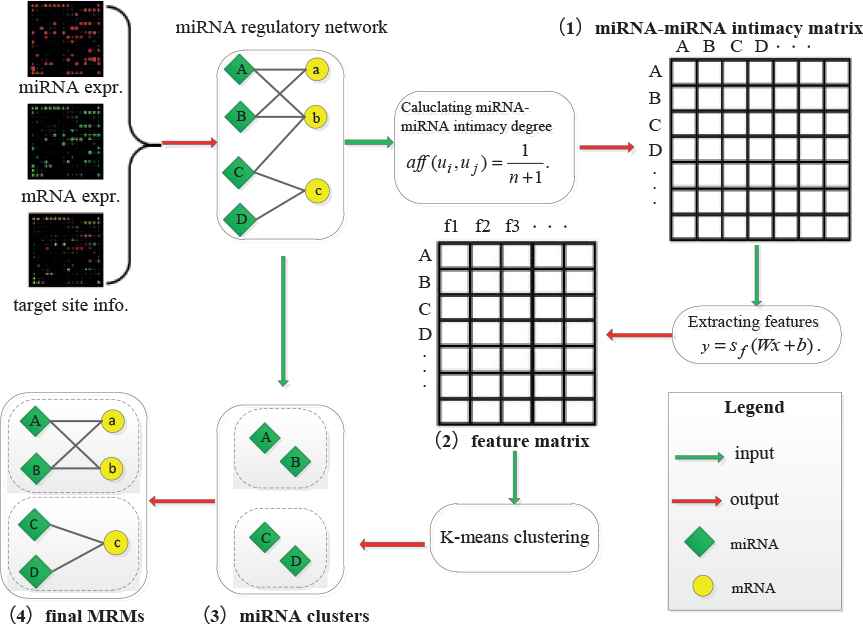
Overview of our proposed framework.
2.1. Building miRNA Regulatory Network
To obtain the reliable relationship between miRNAs and target genes, it is necessary to reduce the false positive in the discovery. In the paper, we employed IDA to predict the causal effect of regulation between miRNAs and mRNAs. Package IDA is available on the website (http://cran.r-project.org/web/packages/pcalg/). Similar to the work of Luo et al. [26], the process consists of three steps: (1) employing the expression information of miRNAs and mRNAs to obtain the causal structure; (2) calculating the causal effects between miRNAs and mRNAs; (3) evaluating the significance of the causal relationship.
We compared IDA with LASSO [27] and Elastic-net [28] by the number of validated interactions they identified. Among the three algorithms, IDA achieved the best overall performance on the three datasets.
2.2. Constructing an Intimacy Matrix
A miRNA regulatory network is a bipartite network that consists of two types of nodes: miRNA and mRNA. In order to facilitate clustering, a bipartite network is typically projected onto an unipartite network [29]. Hence, we convert a miRNA–mRNA regulatory network to a miRNA–miRNA intimacy network (i.e., intimacy matrix) based on the following equation:
Here, ui and uj are two miRNAs, n is the number of passed nodes from ui to uj. For example, in Figure 2, from miRNA A to miRNA D it is necessary to pass b, C, and c. Therefore, the number of nodes from A to D is n = 3. The more the passed nodes, the smaller the intimacy between two miRNAs. The affinity of a node with itself is equal to 1 (i.e., n = 0).
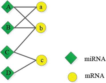
A microRNA (miRNA) regulation network example.
2.3. Extracting High-Level Features
In the previous section, we obtain a miRNA–miRNA intimacy matrix. If we regard each column in the matrix as a dimension, the intimacy between each miRNA and other miRNAs determines its position in the space, and we can cluster adjacent miRNAs. However, the matrix is high dimensional and difficult to clearly express the cluster structure. More importantly, when clustering methods like K-means are utilized to detect modules in these high-dimensional matrices, the results are often low accuracy [30]. Therefore, it is necessary to adopt a low-dimensional way to express the main features of a high-dimensional intimacy matrix.
As a multilayered deep network, SAE [31] can be employed for data dimension reduction. Each layer of SAE is an autoencoder whose outputs are correlated to the inputs of SAE in the preceding layers. These outputs of SAE tend to be gradually smaller to produce a compact representation. The SAE encodes each layer from the first to the last by a deterministic mapping of the equation
On the other hand, SAE can also perform post-to-front decoding of each layer by the following equation:
The second part of Equation (4) is used to reduce the magnitude of the weights to prevent overfitting. Here, λ is a weight decay parameter.
In addition, we also use Kullback–Leibler divergence to enforce a sparsity constraint on the hidden neurons of SAE. Hence the overall SAE loss function is
Here, β is a sparsity penalty factor that determines the weight of the function KL in Equation (5). ρ is the sparsity parameter which represents the frequency of the activation of hidden nodes. And
In this paper, we use SAE to convert the high-dimensional intimacy matrix to a low-dimensional feature matrix. The transformation is described as Figure 3. At the beginning of the process, we train the first hidden layer by using the intimacy matrix X as its input to obtain the primary features. Then, after training the second hidden layer through the primary features, we obtain a group of secondary features. We repeat the similar procedure to train each subsequent layer until the result feature matrix is obtained at the last hidden layer. Finally, we fine-tune the model by employing back-propagation throughout the whole network [32]. The procedure is implemented by software package SAENET which is downloaded from the website (https://cran.r-roject.org/src/contrib/Archive/SAENET/SAENET_1.1.tar.gz).

Feature extraction of microRNA (miRNA) intimacy matrix.
2.4. Clustering miRNAs
In clustering analysis, the best estimate of the number of clusters could be computationally prohibitive due to high computational complexity, which is recognized as the automatic clustering problem [33]. In the last decade, many novel automatic clustering algorithms have been developed, such as ACDE [34], GCUK [35], and so on. However, the algorithms are sometimes difficult to deal with large-scale biological data because of high computational complexity.
There are several factors that make K-means more suitable for clustering the miRNAs. First, compared to some automatic clustering algorithms, K-means is a low computational complexity method. Second, miRNAs with similar function usually co-regulate their target genes [36], which is consistent with the data characteristics of K-means clustering: normally distributed and isotropic. Third, due to the sparsity of miRNA regulatory network, it is difficult to form a very large-scale cluster. The fact that clusters have roughly equal number of miRNAs facilitates K-means clustering. Based on the above analysis, we chose K-means to cluster miRNAs and designed an automatic mechanism to obtain the initial centers of clusters.
Definition 1.
Averaged intimacy of a miRNA aff(ui)
Averaged intimacy of a miRNA is the averaged intimacy value between the miRNA and other N-1 miRNAs in a network. Here, N is the total number of miRNAs in the network. Averaged intimacy of a miRNA ui is defined as
Definition 2.
Averaged intimacy of a set aff
Averaged intimacy of a set is the averaged intimacy value of all nodes in the set, which is defined as
During the clustering process, the miRNAs ui (i = 1, 2, … N) in a feature matrix are sorted in the order of averaged intimacy. By the suggestion of Leskovec et al. [37], the initial centers of K-means should be the nodes that are as far apart as possible from each other. Therefore, a miRNA ui with the smallest intimacy is selected as the first initial center of clusters. Then, for another miRNA uj with the second smallest intimacy, if the expression Equation (8) is true, uj will be selected as the second center. We repeat the process until no node meets the expression Equation (8).
Through the obtained initial centers, we employ K-means to cluster miRNAs. The implementation of K-means in the paper is from the package of R language stats.
2.5. Adding mRNAs into miRNA Clusters
In order to evaluate the intimacy between mRNA and miRNA cluster, we introduce the degree of interaction IND(Ui,vj) for any given miRNA cluster Ui and mRNA vj:
The value of IND indicates the intimacy between mRNA and miRNA cluster, the larger the value is, the closer the two are. We here use this function to determine which miRNA cluster the mRNA should be added into. For example, assuming that there are three edges between mRNA vj and miRNA clusters (i.e., D(vj) = 3). Two of three edges from vj are connected with Ui (i.e., D(Ui, vj) = 2) and only one edge is between vj and Uj (i.e., D(Uj, vj) = 1). Both Ui and Uj consist of four miRNAs, that is, D(Ui) = D(Uj) = 4. According to Equation (9), the IND(Ui, vj) = 1/6 and the IND(Uj, vj) = 1/12. Obviously, the vj has a stronger intimacy with Ui than Uj, therefore the vj will be added into Ui.
Moreover, in order to avoid the identified modules being too large, we only add those mRNAs that are at least co-regulated by two miRNAs in the cluster. So far, we have completed the identification of miRNA regulatory modules. The end result is that each identified module includes miRNAs and its target genes.
2.6. Description of Proposed Framework
The pseudocode for the our proposed framework is outlined in Algorithm 1. The download link for the source code is provided in Appendix A.1.
Algorithm 1: DeMosa detection process
Input: G = (U, V, E), //U: miRNA, V: mRNA, E: edge
n.nodes = 100, //the minimum of node at a layer
dropout = 0.5, //node number decay rate
rel.tol = 0.01 //relative convergence tolerance
Output: M //final MRM set
/***Step 1: constructing intimacy matrix ***/
1: N = len(U)
2: for i = 1 to N
3: count the number of nodes separating two miRNAs
4: building the intimacy matrix X using Equation (1)
5: calculating aff(ui) and aff using Equations (6) and (7)
/***Step 2: extracting high-level features ***/
// calculating the number of units at each hidden
6: nodes = calNumberonLayer(N, n.nodes)
7: fit = SAENET.train (X.train = X, n.nodes = nodes,
lambda = 1e-5, beta = 1e-5,
rho = 0.07, epsilon = 0.1,
max.iterations = 100,
rel.tol = rel.tol)
//feature matrix
8: fmiRNA = fit$X.output
/***Step 3: clustering miRNAs using K-means ***/
9: nodes = {ui sorted by aff(ui), i = 1, 2, …, N}
10: centers = {u1}
11: foreach(uj∈nodes)
12: foreach(ui∈centers)
13: if (aff(uj) ≤ aff & aff(ui, uj) ≤ aff)
14: centers = {centers∪uj}
15: M = kmeans(fmiRNA, centers)
/***Step 4: adding mRNAs into miRNA clusters***/
16: foreach(vj∈V)
//obtaining the index of Mi having the greatest IND(Mi, vj)
17: sn = maxIND(Mi, vj)//D(Mi, vj) ≥ 2
18: Msn = {Msn∪vj}
19: return M
3. EXPERIMENT AND RESULT ANALYSIS
In order to compare the performance of DeMosa, we executed SNMNMF, Mirsynergy, and BCM program codes on the same synthetic and real data sets. The source code files were downloaded from the URLs in their paper (see appendix). We set the relevant parameters for them based on the principles suggested in the papers throughout the experiment. In our model, we set the weight decay parameter λ = 1e-5 since the number of input attributes of our datasets are relatively small. And we set sparsity penalty factor β = 1e-5, sparsity parameter ρ = 0.07, and rel.tol = 0.01 which is the goal that the hidden layer activation aims to achieve. The fine-tuning is an automatic process. The parameter max.iterations is set to 100, which represents the maximum of iterations. The framework proposed in the paper were implemented based on R language (version 3.4.2). These experiments were executed on a machine with an Intel Xeon E5-2609@2.4 GHz CPU and 64 G RAM and the experiment result can be downloaded from the link in Appendix A.1.
3.1. Experiment on Synthetic Datasets
We first employed a computer to generate 100 miRNA regulatory networks consisting of a fixed number of MRMs as benchmark networks, some of them are presented in Figure 4 and Figure S1 in the supplement file. Then, we applied the four algorithms on the networks to compare their clustering accuracy and quality.
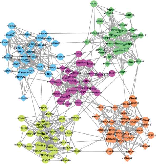
A synthetic microRNA (miRNA) regulatory network sample.
The normalized mutual information (NMI) and modularity Q were chose as the measurement criteria for clustering accuracy and quality. The NMI [38] can be calculated with the equation
Modularity Q is another most widely used evaluation criteria for module quality. Barber [39] defined modularity of a bipartite network as
As shown in Table 1 and Figure 5, DeMosa obtained larger mean values and smaller variances of NMI and Q than the other three methods. The experiment result on the synthetic networks confirmed that DeMosa is superior to the counterparts on the clustering accuracy, stability, and module quality.
| Method | NMI |
Q |
||
|---|---|---|---|---|
| μ | σ | μ | σ | |
| SNMNMF | 0.714 | 0.067 | 0.512 | 0.098 |
| Mirsynergy | 0.774 | 0.045 | 0.552 | 0.078 |
| BCM | 0.723 | 0.071 | 0.525 | 0.108 |
| DeMosa | 0.803 | 0.056 | 0.601 | 0.082 |
μ: mean value; σ: mean variance; NMI: normalized mutual information; BCM: bi-cliques merging.
Overall performance on synthetic datasets.
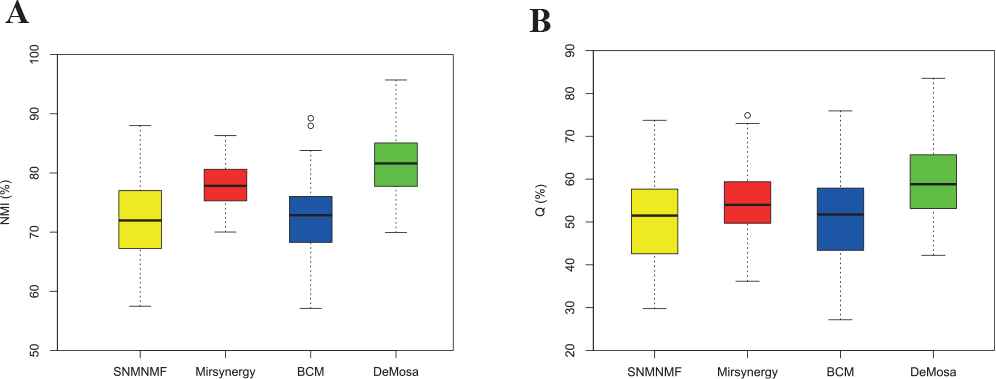
Comparison of normalized mutual information (NMI) and Q for four methods.
3.2. Experiment on Real Cancer Datasets
Three cancer datasets (BRCA, OVCA, and THCA) were exploited to evaluate the performance of our framework. The expression profile data of the cancers were from The Cancer Genome Atlas (TCGA), the target site information of OVCA were downloaded from MicroCosm and the others were downloaded from TargetScan human database [40]. In addition, mean normalization method was implemented to standardize these data. More detail information about obtained miRNA regulatory networks are present in Table 2.
| Dataset | Sample | miRNA | mRNA | Edge |
|---|---|---|---|---|
| BRCA | 331 | 702 | 10,214 | 41,728 |
| OVCA | 385 | 559 | 12,456 | 16,651 |
| THCA | 543 | 710 | 13,306 | 58,892 |
miRNA: microRNA; mRNA: messenger RNA; BRCA: breast cancer; OVCA: ovarian cancer; THCA: thyroid cancer.
The detailed information of miRNA regulatory networks.
We designed three SAEs with different structures to extract high-level features on the datasets (Table 3). There are some differences in the number of layers and nodes for each SAE. Their unit numbers at each hidden layer n.nodes drop by 50% at a time, but not less than 100 to ensure that the features are not too compact. By means of feature extraction, the dimension of an intimacy matrix is greatly reduced. Then, according to the obtained high-level features, we apply K-means to cluster miRNAs.
| Dataset | The Number of Layers | The Number of Nodes |
|---|---|---|
| BRCA | 3 | 702 → 351 → 175 |
| OVCA | 3 | 559 → 280 → 140 |
| THCA | 4 | 710 → 350 → 175 |
BRCA: breast cancer; OVCA: ovarian cancer; THCA: thyroid cancer.
The structure of stacked autoencoder.
After adding mRNAs into miRNA clusters, we detected 29 modules on BRCA, and a module consists of 8.07 miRNAs and 36.55 mRNAs on average. On OVCA and THCA, we detected 42 and 38 modules, respectively (Table 4). Each module consists of 14.33, 8.86 miRNAs and 14.66, 39.11 mRNAs on average, respectively. Notably, the averaged miRNA numbers of each DeMosa MRM are greater than that of SNMNMF, Mirsynergy, and BCM on the three datasets. We further compared the density of the identified MRMs. DeMosa-MRMs are not denser than BCM, but significantly more densely connected as compared to SMNMNF and Mirsynergy. Besides, the averaged MMEC (miRNA–MRNA Expression Correlation) [12] of DeMosa-MRMs are −0.544, −0.233, and −0.523, respectively, which are less than the MRMs detected by the other methods. Through statistical analysis, we found that DeMosa can gather more negative correlated and densely connected modules than its counterparts on BRCA, OVCA, and THCA. More details of all DeMosa-modules are provided in supplementary file Table S1. The graphical representation of some DeMosa-modules are presented in Figure S2 in the supplementary pdf file.
| Cancer | Method | Num | AmiR | AmR | Dens | MF | MMEC |
|---|---|---|---|---|---|---|---|
| BRCA | SNMNMF | 39 | 2.62 | 71.56 | 0.047 | 2 | −0.045 |
| Mirsynergy | 53 | 5.77 | 24.15 | 0.03 | 10 | −0.08 | |
| BCM | 43 | 5.65 | 28.37 | 0.28 | 15 | −0.15 | |
| DeMosa | 29 | 8.07 | 36.55 | 0.191 | 6 | −0.544 | |
| OVCA | SNMNMF | 49 | 4.12 | 81.37 | 0.003 | 6 | 0.052 |
| Mirsynergy | 84 | 4.76 | 7.57 | 0.39 | 12 | −0.37 | |
| BCM | 36 | 2.08 | 2.28 | 0.99 | 8 | 0.24 | |
| DeMosa | 42 | 14.33 | 14.66 | 0.363 | 10 | −0.233 | |
| THCA | SNMNMF | 39 | 2.34 | 74.82 | 0.028 | 7 | −0.008 |
| Mirsynergy | 50 | 7.60 | 32.26 | 0.02 | 7 | −0.08 | |
| BCM | 41 | 8.07 | 14.29 | 0.16 | 13 | −0.11 | |
| DeMosa | 38 | 8.86 | 39.11 | 0.190 | 8 | −0.523 |
Num: module number; AmiR and AmR: averaged miRNA and mRNA number per module; Dens: averaged density per module; MF: MRMs enriched in miRNA families; MMEC: averaged miRNA-mRNA expression correlation; BRCA: breast cancer; OVCA: ovarian cancer; THCA: thyroid cancer; BCM: bi-cliques merging.
Overall comparison among the four methods.
3.2.1. Analyzing structure of MRMs
To explore synergistic regulation within MRMs, we herein analyze the density of each MRM to detail the connectivity between miRNAs and genes. As illustrated in Figure 6, the density distributions of MRMs detected by the four approaches are significantly different. The MRMs identified by DeMosa and BCM are more densely connected than other two methods. SNMNMF-MRMs are generally sparse on the three datasets. Mirsynergy only detected some densely connected modules on OVCA dataset. Although BCM-MRMs have the largest averaged density, on the OVCA dataset it only clustered a small amount of miRNAs and mRNAs (Table 4).
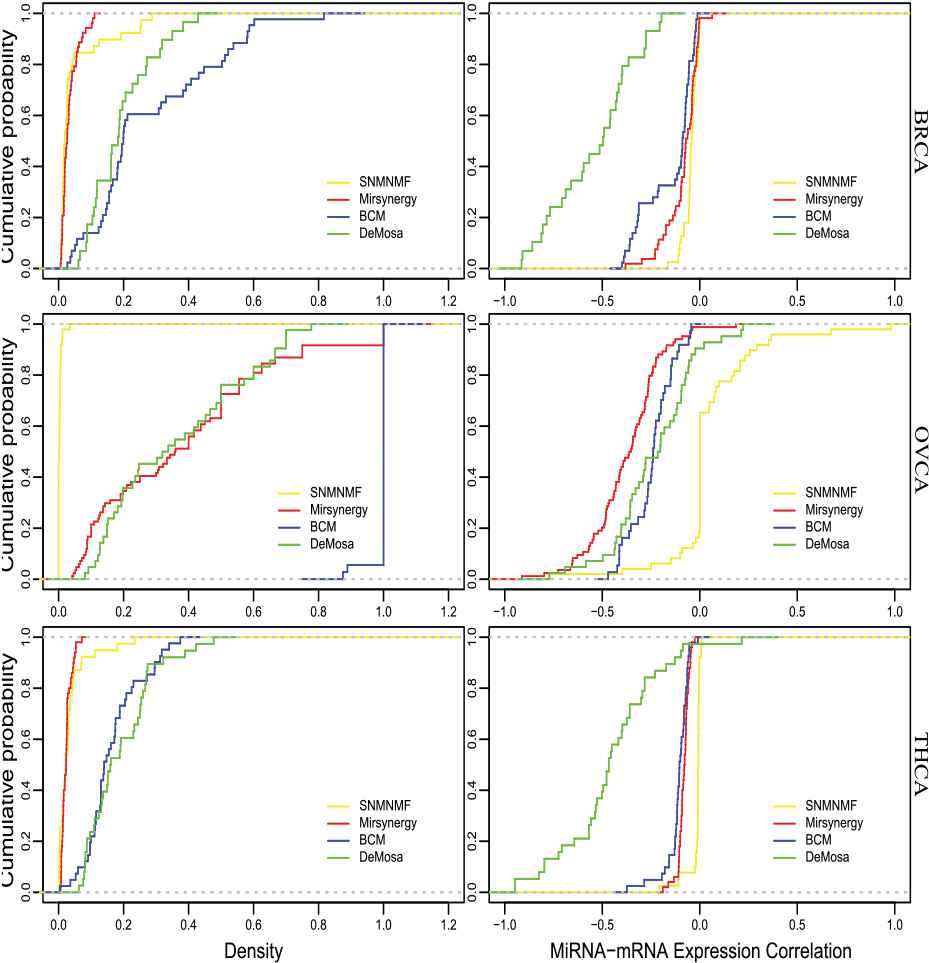
Cumulative Distribution Function (CDF) diagram for density and miRNA–mRNA expression correlation (MMEC) of microRNA regulatory modules (MRMs).
Moreover, we also compared the regulation strength between miRNAs and mRNAs within the MRMs through MMEC of the identified MRMs. The negative correlation of DeMosa-MRMs are smaller than that of the MRMs detected by the other three methods except Mirsynergy-MRMs on the OVCA dataset.
The above analyses indicate that Demosa has the capacity to detect denser and more strongly regulated MRMs, while that of the other methods vary significantly with the datasets. Density versus MMEC scatter plots are provided in the supplement file Figure S3. All scatter plots of the expression correlations of DeMosa-MRMs from the three cancer are also provided in the supplementary file Figures S4–S6.
3.2.2. Comparing the execution time
The time complexity of four-step method DeMosa is O(N2+ KTN + KM). Step I takes O(N2) to construct intimacy matrix, where N is the number of miRNAs. Step II takes O(Ncd) to extract higher level features [41], where d is the maximum number of hidden layer nodes in SAE, and c is the average degree of the network. On the three cancer datasets, the averaged degree of the mRNAs are 4.09, 1.34, and 4.42, respectively. From Tables 2 and 3, we can see that c and d don't increase significantly with N. Therefore, c and d can be regarded as some constants. Step III takes O(KTN) to cluster miRNAs by K-means, where K represents the number of cluster centers and T represents the number of iterations. Step IV takes O(KM) into add M mRNAs to K miRNA clusters.
The time complexity of our framework is smaller than O(KT(S + M + N)2) of SNMNMF, O(M(N + M)) of Mirsynergy, and O(B(N + M)3) of BCM. Here, N and M represent the number of miRNAs and their genes, T the maximum of iterations, K the number of clusters, and B the number of Bi-cliques [42]. The minutes the four methods took on the three cancer datasets are shown in Table 5.
| Method | BRCA | OVCA | THCA |
|---|---|---|---|
| SNMNMF | 35 | 25 | 40 |
| Mirsynergy | 30 | 25 | 35 |
| BCM | 55 | 45 | 65 |
| DeMosa | 29 | 23 | 35 |
BRCA: breast cancer; OVCA: ovarian cancer; THCA: thyroid cancer; BCM: bi-cliques merging.
The number of minutes the four methods took.
3.2.3. Evaluating synergy of miRNAs
We here conducted miRNA family enrichment analysis to evaluate miRNA synergy in DeMosa-MRMs. Family classification data of miRNA was downloaded from the website (http://www.mirbase.org/). We counted the MRMs enriched in one or more miRNA families for the two algorithms by hypergeometric test (q-value < 0.05). As shown in Table 4, for BRCA/OVCA/THCA, 6/10/8 of DeMosa-MRMs are enriched in one or more miRNA families. Except SNMNMF, the other two methods also achieved good enrichment effect. All DeMosa-MRMs from BRCA enriched in miRNA families are shown in Table 6. The lists of all DeMosa-MRMs from three cancers enriched in miRNA families are provided in the supplementary materials (Table S2).
| MRM | miRNA | miRNA Family |
|---|---|---|
| 4 | miR-518b, miR-518c, miR-518f, miR-520e | MIPF0000019 |
| 5 | miR-27a, miR-27b | MIPF0000036 |
| 7 | miR-300, miR-381 | MIPF0000018 |
| 13 | let-7b, let-7c, let-7i | MIPF0000002 |
| 18 | miR-30a, miR-30b | MIPF0000005 |
| 22 | miR-30a, miR-30d, miR-30e | MIPF0000005 |
| 22 | miR-130b, miR-301b | MIPF0000034 |
| 22 | miR-519d, miR-519e | MIPF0000020 |
MRM: the index of MRM; miRNA: miRNAs in a MRM; miRNA Family: miRNA families enriched in a MRM; BRCA: breast cancer.
DeMosa-MRMs from BRCA enriched in miRNA families.
3.2.4. Exploring correlation between miRNAs and cancers
To investigate the role of miRNAs as tumor markers to diagnosis tumors, we carry out miRNA-disease correlation analysis for the MRMs on OVCA dataset. The cancer related miRNA benchmark dataset is from miRCancer (http://mircancer.ecu.edu/). The OVCA benchmark dataset is comprised of 121 onco-miRNAs. Excitingly, 70 onco-miRNAs from OVCA benchmark dataset were detected in DeMosa-MRMs (Table 7). In addition, there were 41 MRMs containing onco-miRNAs (onco-MRMs). DeMosa-MRMs are superior to the counterparts in both PmiR (the proportion of recalled onco-miRNAs) and PMRM (the proportion of onco-MRMs). Therefore, DeMosa-MRMs can help us diagnose cancers more accurately than the MRMs detected by the other methods. All onco-miRNAs enriched in DeMosa-MRMs on three datasets are provided in the supplementary file (Table S3).
| Method | OncoMiR | PmiR | OncoMRM | PMRM |
|---|---|---|---|---|
| SNMNMF | 60 | 49.59% | 38 | 77.55% |
| Mirsynergy | 56 | 54.90% | 68 | 80.95% |
| BCM | 25 | 24.51% | 25 | 69.44% |
| DeMosa | 70 | 57.85% | 41 | 97.62% |
OncoMiR: onco-miRNAs; PmiR: The percent of recalled onco-miRNA; OncoMRM: The MRMs having onco-miRNAs; PMRM: The percent of onco-MRM; BCM: bi-cliques merging.
Onco-miRNA enrichment profile of the four methods on OVCA dataset.
Figure 7 illustrates averaged expression values of 43 DeMosa-MRMs from OVCA and 12 miRNAs from DeMosa-MRM 34. From the two heatmaps, we can effectively differentiate cancer patients and normal samples through the detected DeMosa-MRMs and miRNAs.
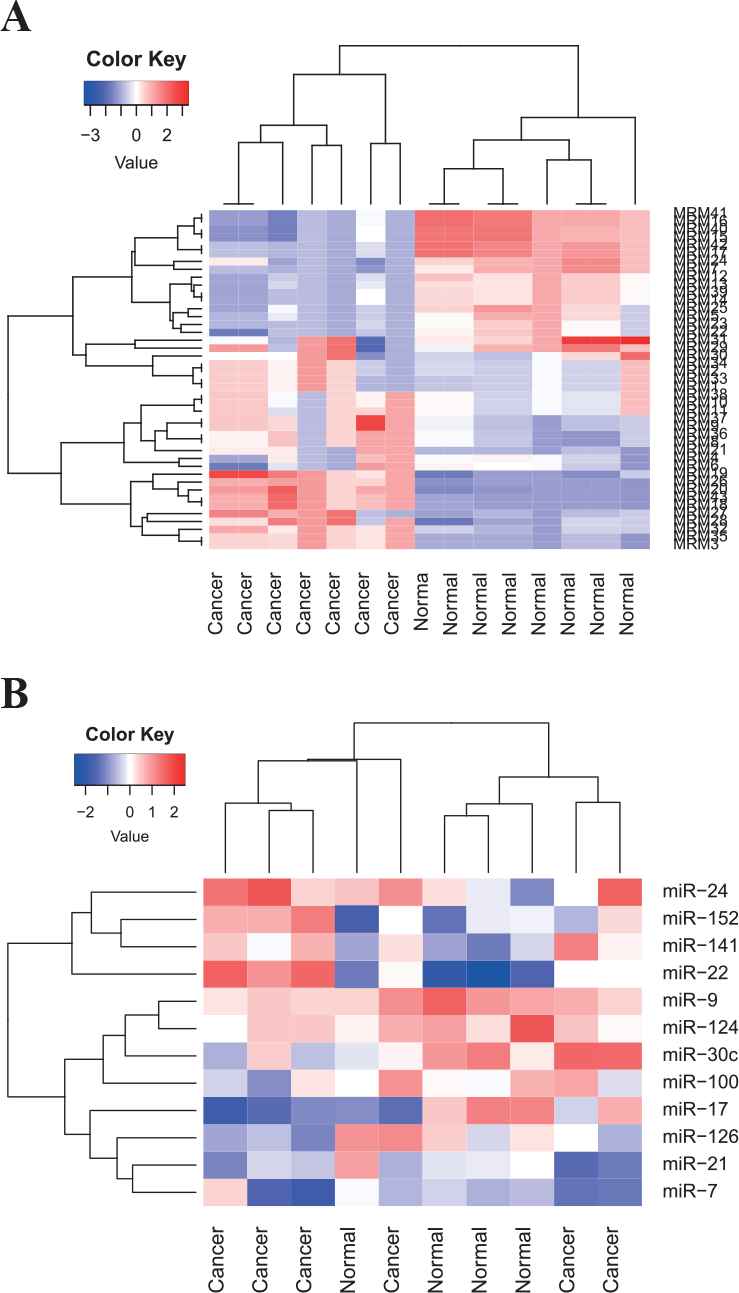
Heatmaps of 43 DeMosa-microRNA regulatory modules (MRMs) and 12 microRNA (miRNAs) from DeMosa-ovarian cancer (OVCA)-MRM 34.
3.2.5. Verifying diagnostic ability of MRMs
To examine the diagnostic ability of DeMosa-MRMs, we first divided the samples from TCGA clinical data into two groups. High expression group represents patients with higher miRNA expression level than the mean miRNA expression, and low expression group is the rest. We then applied Kaplan–Meier approach to analyze the survival characteristics of them. We observed that DeMosa-MRMs present significantly different survival rates (FDR < 0.1) (Figure 8). High expression group patients (red curve) in the three modules suffered higher risk.
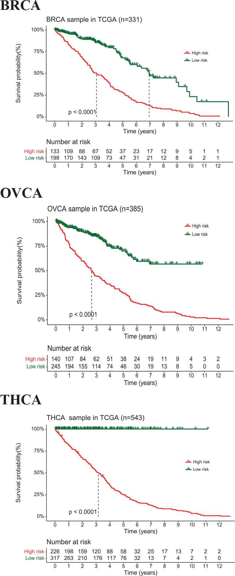
Kaplan–Meier survival analyses by DeMosa-microRNA regulatory module (MRMs).
4. CONCLUSION
In this paper, we applied the deep-learning-based framework DeMosa to detect MRMs. We first constructed miRNA intimacy matrix based on the path length between two miNRAs, by which the initial centers were automatically determined to improve the efficiency of K-means clustering. Then, we employed SAE to extract high-level features of the obtained intimacy matrix. After that, we detected miRNA clusters by K-means. Finally, we added the strongly correlated target genes to corresponding miRNA clusters to obtain final DeMosa-MRMs. Moreover, we compared with other three methods on different datasets. A brief comparison of the potential benefits and drawbacks of four methods is summarized in Table 8.
| Method | Peculiarities | Benefits | Drawbacks |
|---|---|---|---|
| SNMNMF | Nonnegative matrix factorization | Good performance on dimension reduction | Predefining number of MRM; clustering unrelated miRNAs and mRNAs |
| Mirsynergy | Maximizing synergy of miRNAs | Better functional synergy | Predefining weight of network; large-scale MRMs |
| BCM | Bi-cliques merging | Denser MRMs | Predefining density thresholds; small-scale MRMs |
| DeMosa | Extracting high-level features | Balance between function and structure | Fine-tuning SAE |
BCM: bi-cliques merging; SAE: stacked autoencoder; miRNA: mMicroRNA; MRM: mMicroRNA regulatory module; mRNA: mMessenger RNA.
Comparing the qualities of the four methods.
It is important to emphasize that DeMosa is more suitable for a variety of different scenarios than its counterparts. The clustering quality of DeMosa was examined on computer generated networks with obvious network structures. The clustering results confirmed that DeMosa boasts higher NMI and Q values than other three methods. DeMosa was also tested on BRCA/OVCA/THCA datasets and the experiment demonstrated that DeMosa has the capacity to detect more strongly correlated and higher diagnostic value modules. In conclusion, DeMosa has the potential power to detect MRMs on various complex biological networks. In future work, DeMosa will improve the effectiveness and efficiency of extracting high-level features from an intimacy matrix.
CONFLICT OF INTEREST
The authors declare no conflict of interest.
AUTHORS' CONTRIBUTIONS
Yi Yang conceived, designed, and performed the experiments; Yan Song contributed materials/analysis tools; Yi Yang wrote the paper; Yi Yang and yan Song reviewed the paper.
ACKNOWLEDGMENTS
The research is funded by the Scientific Research Key Project of Education Department of Hunan Province of China (Grant No.18A470).
APPENDIX
A.1. Source Code and Experiment Result
The source code files and supplementary data for DeMosa are available at https://github.com/snryou/DeMosa
A.2. Some Acronyms in the Paper
| Index | Acronym | Expression |
|---|---|---|
| 1 | BRCA | Breast cancer |
| 2 | miRNA | MicroRNA |
| 3 | MRM | MicroRNA regulatory module |
| 4 | mRNA | Messenger RNA |
| 5 | MMEC | miRNA–mRNA expression correlation |
| 6 | NMI | Normalized mutual information |
| 7 | OVCA | Ovarian cancer |
| 8 | Q | Modularity |
| 9 | SAE | Stacked autoecoder |
| 10 | THCA | Thyroid cancer |
REFERENCES
Cite this article
TY  - JOUR
AU  - Yi Yang
AU  - Yan Song
PY  - 2019
DA  - 2019/07/18
TI  - A Stacked Autoencoder-Based miRNA Regulatory Module Detection Framework
JO  - International Journal of Computational Intelligence Systems
SP  - 822
EP  - 832
VL  - 12
IS  - 2
SN  - 1875-6883
UR  - https://doi.org/10.2991/ijcis.d.190718.002
DO  - 10.2991/ijcis.d.190718.002
ID  - Yang2019
ER  -