
II-Learn—A Novel Metric for Measuring the Intelligence Increase and Evolution of Artificial Learning Systems
- DOI
- 10.2991/ijcis.d.191101.001How to use a DOI?
- Keywords
- Machine learning; Machine intelligence; Intelligent system; Evolving system; Cooperative multiagent system; Machine intelligence measure
- Abstract
A novel accurate and robust metric called II-Learn for measuring the increase of intelligence of a system after a learning process is proposed. We define evolving learning systems, as systems that are able to make at least one measurable evolutionary step by learning. To prove the effectiveness of the metric we performed a case study, using a learning system. The universality of II-Learn is based on the fact that it does not depend on the architecture of the studied system.
- Copyright
- © 2019 The Authors. Published by Atlantis Press SARL.
- Open Access
- This is an open access article distributed under the CC BY-NC 4.0 license (http://creativecommons.org/licenses/by-nc/4.0/).
1. INTRODUCTION
Intelligent systems have been successfully applied for the solution of a variety of difficult practical problems, such as medical diagnosis [1–6], intrusion detection [7], network traffic anomalies detection [8], multisensor battlefield reconnaissance simulation [9], local semantic indexing for resource discovery on overlay networks [10], distributed reasoning for context-aware service [11] and real-time water demand management [12]. Given a problem, its solving difficulty can be considered from different viewpoints, for example, from the human and the computational viewpoint. In this paper, we focus on difficult problems from the computational viewpoint, such as NP-hard problems.
Many intelligent systems are agent-based (ABSs) [13–20], consisting of intelligent agents (IAs) and intelligent cooperative multiagent systems (intelligent CMASs). There is no unanimous definition of intelligent agent-based systems (IABSs) [13,14,21–23]. Frequently, the characterization of a system as intelligent is based on its ability to learn autonomously a specific task. Learning can result in the modification of existing knowledge, or even in the construction or discovery of new knowledge.
The appreciation/definition of intelligence of a system is usually based on bio-inspired considerations [13–15,24–26] including autonomous learning, self-adaptation, and evolution. A variety of machine-learning approaches for solving practical problems have been proposed [27–38] varying from simple to complex techniques. Rote learning is an example of simple learning. For humans, rote learning consists in memorization based on repetition, while many early expert systems can be considered as rote learners since knowledge is retained in the form transmitted by a human supervisor without any modification. For example, MYCIN [39] could be considered as such a system capable of solving problems similarly with the human specialists in the context of decision support system for infectious disease management. More complex learning examples may include reasoning approaches, such as induction and abduction.
Must be mentioned that if a system learns, it does not necessarily mean that it has become more intelligent, in the sense that it has a measurable increase in the intelligence level. Learning in some cases could result even in a decrease of intelligence, for example, a system could learn misleading data or overfit on the training data thus losing its ability to generalize. Furthermore, we consider that the intelligence measure modification (increment or decrement in some cases), does not directly relate to the learning complexity. Even a very simple form of autonomous learning, such as rote learning, can result in a significant increase (e.g., of the performance) and sometimes even of the intelligence [40].
The main contribution of this paper is the introduction of a novel universal mathematically grounded metric, called II-Learn (metric for measuring the Intelligence Increase of artificial Learning systems), that is able to quantify the Central Intelligence Tendency (CIT) and provide additional characterization of a system's intelligence. The calculation of II-Learn metric considers the CIT of the intelligent system before and after the learning process and makes an accurate comparison by verifying if the two measured central intelligence tendencies are different from the statistical viewpoint, taking into consideration the variability in the practical problem-solving intelligence. The proposed approach provides both enhanced robustness, accuracy and universality over most current approaches.
In a previous study the universal and robust MetrIntComp metric [41] for the measurement of system's intelligence was proposed. Since both metrics II-Learn and MetrIntComp quantify the problem-solving intelligence of systems, they can be considered comparable. The main advantage of II-Learn over the MetrIntComp consists in its higher accuracy. II-Learn conserve the robustness property of the MetrIntComp metric by making some kind of experimental problem-solving intelligence evaluation data transformation. II-Learn consider the presence of possible extremes (measured problem-solving intelligence values that are very different from the other measured problem-solving intelligence values) and it applies a methodology to remove them.
Furthermore, we introduce definitions for a variety of concepts, which include the “Evolutionary Step” in the life cycle of an intelligent learning system, the “Involutionary Step” in the life cycle of an intelligent learning system, and respective system definitions that include the “Intelligent Evolving Learning System” and the “Intelligent Involving Learning System.” II-Learn metric enables the verification if a studied system attained an evolution in intelligence by learning, in the sense of intelligence increase (such systems are referred as Evolving Intelligent Learning Systems) or intelligence decrease, called involution in intelligence (such systems are referred as Involving Intelligent Learning Systems). In nature the most frequent situation of what we call “involution” is when a species move into another environment or during a longer time evolution stops using some senses/structures for surviving; however, these senses/structures may decrease or even disappear. For example, we mention the wings of ostriches as they are remnants of their flying ancestors' wings. II-Learn enables accurate measurements, even in the case of a small modification of a system's intelligence, and it takes into consideration the variability in the problem-solving intelligence level. Thus it can be used in the context of a cooperative multiagent system that could manifest different levels of intelligence for different problems undertaken for solving.
To demonstrate the effectiveness of II-Learn we performed an experimental case study, using a cooperative multiagent system specialized in solving the Travelling Salesman Problem (TSP) [42,43] that is a well-known NP-hard problem. We investigate whether a simple rote learning of a system that exhibits a behavioral adaptation by learning results in an intelligence increase, and in the affirmative case if an evolutionary step in the intelligence is performed.
The rest of this paper is organized in 6 sections. Section 2 discusses the motivation of this work with respect to open issues identified in literature; presents the state-of-the-art metrics/methods proposed for measuring machine intelligence. In Section 3 the proposed II-Learn metric is presented. Section 4 presents an experimental study that demonstrates and validates II-Learn metric. Section 5 provides a discussion about the proposed metric, and finally, Section 6 summarizes the main conclusions of the presented research.
2. STATE-OF-THE-ART AND MOTIVATION
ABSs frequently enable intelligent solving of a large diversity of real-life difficult problems, like, optimization of coordination of human groups online [44], and collaborative multisensor agents for multitarget tracking and surveillance [45]. Although several studies address intelligent problem-solving using ABSs, the evidence provided for their intelligence is usually intuitive, and there are several still open issues with respect to measures used for the assessment of their learning ability.
2.1. Evidence of System Intelligence
In the case of cooperative multiagent systems generally, both learning and intelligence measurement could be even more complex than in the case of non-cooperative intelligent systems. Usually, cooperative multiagent systems are presented to be intelligent, based on the consideration that the cooperation between individual (even very simple) agents results in the emergence of intelligence at the level of the whole system [46,47]. This is the definition of intelligence that we adopt in our research. Such a simple consideration is just intuitive without offering evidence of intelligence, in terms of a measure that quantifies the level of intelligence.
For example, Yang et al. [48] presented an intelligent mobile multiagent system composed of simple reactive agents endowed with knowledge retained as a set of rules describing network administration tasks. This cooperative multiagent system could be considered as intelligent based on the intuitive motivation that it mimics the behavior of a human network administrator, who acts in an intelligent way as a human specialist. However, that study neither provided a quantitative measure to the intelligence of the cooperative multiagent system, nor an effective numerical comparison of a system's intelligence with the intelligence of another system.
Machine learning frequently is presented as a successful approach for different problems solving even in very recent studies and researches [49–51]. This proves that computing systems, including ABSs could use such learning techniques in order to solve efficiently problems. In the mentioned works and many others, the way how the learning leads to effective improvements is not effectively proved or even studied. Paper [49] presents a survey on supervised machine-learning techniques that lead to efficient automatic text classification. In [50] a smart adaptive run parameterization enhancement of user manual selection of running parameters in fluid dynamic simulations using machine-learning techniques is proposed. Paper [51] proposes a machine-learning approach to identify multimodal MRI patterns predictive of isocitrate dehydrogenase and 1p/19q status in diffuse low- and high-grade gliomas.
There are very few studies and researches that formulate the pertinent and important research question, if the learning does not have any kind of effect, or even worst it could lead as result decreases or errors. In the research [52] it is studied the problem of inclusion of machine-learning components (MLCs) in cyber-physical systems (CPSs). In case of such a CPS, the researchers state that the operation correctness could depends even in a high degree on the incorporated MLC(s). In this context, it was formulated the research question: “Can the output from learning components lead to a failure of the entire CPS?” As a practical application, the problem of falsifying signal temporal logic specifications for CPS endowed with MLC(s) is addressed. According to this requirement, it is proposed a compositional falsification framework. The effectiveness of the technique that is proposed is proved on an automatic emergency braking system that is endowed with a perception analysis based on deep neural networks component.
Another study [53] investigated the subject of inconsistent data, that appear as outliers, which can be learned by a diagnosis system if is not identified and deleted. Such data could have a negative effect to accuracy and performance of the diagnosis system. For outlier data identification a k-Nearest Neighbor (k-NN) method was applied.
Knowing the fact that the learning process does not have an effect or it could lead to a decrease or apparition of errors, it may be helpful to take a different solution in order to avoid such effects, like analyzing the result of this learning process, if there is a chance to lead to a malfunction for example.
2.2. Learning Ability Assessment
An important aspect in the study of learning systems is the assessment of their ability to learn. In this paper, we investigate an approach to measure if learning can lead to a measurable increase in the intelligence level. It should be noted that if a system learns, it does not necessarily mean that it has become more intelligent, in the sense that it has a measurable increase in the intelligence level. Learning in some cases could result even in a decrease of intelligence, for example, a system could learn misleading data or overfit on the training data thus losing its ability to generalize. Furthermore, we consider that the intelligence measure modification (increment or decrement in some cases), does not directly relate to the learning complexity. Even a very simple form of autonomous learning, such as rote learning, can result in a significant increase (e.g., of the performance), and sometimes even of the intelligence [40].
We consider intelligence level measuring of a CMAS based on difficult problem-solving ability. An intelligence increase can be quantified by a measurable increase of the problem-solving ability/intelligence, whereas an intelligence decrease can be quantified by a measurable decrease of the problem-solving ability/intelligence. In order to further explain the notion of difficulty and intelligence increase or decrease in problem-solving, as an example, let us consider a simplified scenario of an intelligent medical diagnosis system that is able to learn. The intelligent system is specialized in the solving of a very difficult diagnosis problem, for example, an illness for which the establishment of an effective treatment is very difficult. In this context, the variability of intelligence can be associated with the selection of a specific treatment that could be more or less effective. An intelligence increase can be associated with the elaboration of more effective treatments, whereas an intelligence decrease can be associated with the elaboration of less effective treatments.
A problem with a specific type could be solved by a variety of CMASs with different architectures. Even if we consider a particular domain of knowledge there are a lot of solvable problems by computing systems with a wide diversity of types and complexity. This motivates the necessity to design universal metrics for measuring machine intelligence. However to date, as it is also pinpointed in the review study presented in the next sections, current metrics have limitations in their universality.
2.3. Metrics for Measuring Machine Intelligence
In 1950, Alan Turing [54], considered a computing system as intelligent, if a human assessor could not decide the nature of the system (being human or otherwise) based on questions asked from a hidden room. We consider that the biological and Artificial Intelligence (AI) are different in nature; therefore, they should not be compared directly. Although Turing's test was an early theoretical proposal in AI; we consider it as a good starting point for the design of metrics/methods enabling the comparison of intelligence of two systems by the same type (biological or artificial). Some milestones of AI could be clearly set this way, for example, using metrics to assess intelligence in competitions between systems and humans, such as the well-known competition between the chess machine named Deep Blue and the chess master Garry Kasparov [55], and between the IBM Watson computing system and human experts in the game named Jeopardy [56]. Schreiner [57] accentuated the necessity of creating metrics for measuring the systems' intelligence in a study performed for the US National Institute of Standards and Technology and proposed relevant measurement and comparison approaches.
Legg and Hutter [58] studied a number of well-known definitions of human intelligence and extracted their essential features. These were then mathematically formalized in order to produce a general measure of machine intelligence. The authors showed that this formally defined measure is related to the theory called universal optimal learning agents. Hibbard [59] proposed a novel metric for measuring an agents' intelligence, which is based on the theory/principle of the hierarchy of sets of increasingly difficult environments. Hibbard considers an agent's intelligence measurement according to the ordinal of the most difficult set of environments that may occur. The metric proposed in that work includes the number of time steps required for an agent to pass the test.
Hernandez-Orallo and Dowe [60] proposed the idea of universal anytime intelligence test. They considered that such a test should be universal in the sense that could be able to measure intelligence, in a wide variety of situations that include even very low or very high intelligence. Their proposal was based on the so-called C-tests and compression-enhanced Turing tests that were designed in the late 1990s. In that study, a synthesis of different state-of-the-art tests was performed, highlighting their limitations.
Sometimes the agents' intelligence is considered based on the complexity of the problems that they are able to solve. Anthon and Jannett [61] investigated the intelligence measuring appropriateness of the agent-based systems based on the ability to compare different alternatives considering their complexity. In their experimental setup, a distributed sensor network system was considered. This approach was tested by comparing an intelligence measure in different agent-based scenarios.
Winklerova [62] assessed the collective intelligence of a particle swarm optimization system according to a novel Maturity Model. The proposed approach was based on the Maturity Model of Command and Control operational space and the model of Collaborating Software. The main aim of that study was to obtain a more thorough explanation of how the intelligent behavior of the particle swarm emerges.
Franklin and Abrao [63] proposed an introductory methodology for the agent's intelligence testing. This methodology is based on the calculation of a proposed general intelligence factor and the theory of multiple human intelligences [64]. A set of tests assessed the multiple intelligences of the agents, by analyzing their problem-solving behavior in different situations. The proposed approach was intended for both qualitative and quantitative evaluations of intelligence.
In [65] we proposed an innovative metric called MetrIntPair (Metric for Pairwise Intelligence Comparison of Agent-Based Systems) for comparison of two cooperative multiagent systems problem-solving intelligence. MetrIntPair is able to make an accurate comparison by taking into consideration the variability in the problem-solving intelligence of systems. Two intelligent systems with the same intelligence can be included in the same class of intelligence. The design of metrics that are able to make differentiation of systems in problem-solving with respect to their intelligence is a very important subject since they can be used to select the system that is able to solve a particular problem in the most intelligent way.
In [66] we proposed a metric called MetrIntMeas (Metric for the Intelligence Measuring) for measurement of the intelligence of a swarm system for difficult problem-solving. MetrIntMeas is an accurate and robust metric enabling at an application the classification based on the intelligence of a studied swam system. It is able to verify if a studied swarm system belongs to the same class with the systems which have a specific reference intelligence value. In that paper, the intelligent evolving systems were defined stating that the evolution in the intelligence of a swarm system should be measured by using the MetrIntMeas metric.
In [67] we highlighted the fact that the identification of intelligent systems (not particularly intelligent learning systems) with extremely-low or extremely-high, outlier, intelligence is an important subject, and we proposed a method called OutIntSys for the detection of systems with high and low outlier machine intelligence from a set of studied intelligent systems. We consider that the treating of outliers is a very important subject even in the case of metrics for measuring the intelligence of learning systems. Outlier values could have a negative influence on the accuracy of the intelligence measurements.
In our previous studies [65,66] we highlighted the fact that a metric for intelligence measurement needs to treat the aspect of variability in intelligence. The metrics presented in [65,66] are illustrative to the situation where the treatment of the variability by a metric can result in advantages to the accuracy and robustness in intelligence level comparison and classification of the systems based on their intelligence. A disadvantage of many previously proposed intelligence metrics in the literature consists of limited universality. Universality provides advantages including independence of the metric from the measured agent/cooperative multiagent system architecture, the environment in which the system operates, and other influencing factors. Metrics proposed in the literature are designed based on different kind of considerations/principles; therefore, most of them cannot be effectively compared with each other.
The literature review performed in this section reveals that there is no unanimous viewpoint related to what a metric for measuring the intelligence should measure. There is no accepted standardization related to intelligence measurement. Most intelligent systems are able to learn. The design of effective metrics for artificial learning systems is necessary. We consider that a metric for measuring machine intelligence must conserve the very important properties by universality, accuracy and robustness. In the case of an intelligent learning system under investigation, such a metric should be useful at least in the following processing/analysis tasks: 1) to measure the intelligence of the system before a learning process; 2) to measure the intelligence of the system after a learning process; 3) to verify if the learning process results in any modification in intelligence level; 4) to be able to verify accurately even small changes in intelligence.
We would like to outline that a measurable improvement by learning does not necessary means an increase in the intelligence. There are very few studies focusing on the effect of modification of the intelligence as a consequence of learning [68,69]. There are no studies explicitly focusing on the design of metrics able to verify accurately (taking into consideration the variability in the intelligence) that even small changes, as result of learning, can have as an effect an evolutionary or involutionary step in intelligence.
3. THE PROPOSED II-LEARN METRIC
In order to cope with the afore-mentioned open issues, we propose II-Learn metric, which can be used to provide quantifiable evidence of intelligence, suitable for assessing the intelligence increase of a cooperative multiagent system by learning, while conserving universality and providing enhanced accuracy and robustness. In the following we describe this metric after the introduction of the explanation of the principle and the formalism on which it is based on.
3.1. Principle
There are many studies and researches [46–48] that define CMASs composed of extremely simple agents as intelligent based on the efficient, flexible and robust cooperative problem-solving. It is considered the intelligence as emergent at the system's level. Frequently the autonomous learning capacity is associated with the intelligence of a system. In our approach we are focused on CMASs where intelligence emerges at the system's level, that are able to learn. The rationale of the metric that we propose is to measure if by learning a studied CMAS evolved in intelligence. In our approach, the intelligence of such a considered CMAS must allow the solving of very difficult problems. We consider the principle of cooperative multiagent system's intelligence level measuring based on the advanced ability to solve difficult problems. The difficult problem-solving ability is considered as the intelligence level measure.
3.2. Formalism
In our approach, it is considered the measuring of a specific type of intelligence considered by interest to a human evaluator (HE) who is a specialist in machine intelligence science.
Different studies discuss human specialist who acts as evaluators. Paper [70] presents a methodology for analysis of different kind of human errors. The US Patent [71] proposes a general approach to some methods for presentation and evaluation of constructed responses assessed by the HEs. In [72] is investigated the HE in image enhancement tasks with the purpose to make visual improvements of images. Paper [73] study the perceived value of two designed sentiment analysis tools for understanding the Finnish language, in contrast to HEs. In [74] the principal role of HEs is analyzed in the applied automatic semantic technologies.
In our approach HE is responsible to measure if a CMAS system's intelligence level increased as a result of learning by using the II-Learn metric. A problem-solving intelligence evaluation result by the considered type is expressed as a so-called intelligence indicator value. An intelligence indicator value is based on a specific calculus performed on an experimental problem-solving intelligence evaluation. In order to illustrate the previously introduced notions, we provide the following a scenario.
Let us consider an intelligent CMAS denoted CoopRob composed of robotic agents able to pilot cooperative transport cars. The agents must cooperatively perform different missions established by a human specialist(s) denoted HE. The first type of mission consists of the transportation of a set of objects to established destinations. The task of distribution of a larger set of objects to different destinations is undertaken for solving by the transport cars. A type of problems to cope with this situation can be the TSP. The latter type of problems consists in the collection of a set of objects from distributed sources that are established or they should be found/discovered. Based on the efficient cooperative solving of difficult problems the intelligence can be considered at the cooperative system's level. The intelligence of such a system cannot be unanimously defined. The human specialist(s) who would like to measure the intelligence of CoopRob must define what type of intelligence he/she would like to measure. The intelligence can be considered based on different particular or general considerations/principles (or their combination), such as advanced ability to collect objects or advanced ability to distribute objects. HE should establish the corresponding calculus of problem-solving intelligence indicator value that corresponds to the type of intelligence by interest.
Our approach includes a calculus of the so-called CIT before the learning process and after the learning process. The CITs of a learning system before and after learning are not absolute measure; they are based on the calculated intelligence indicator values obtained as the result of the problem-solving intelligence evaluations. Along with the CITs some other calculated indicators, which characterize the intelligence level are computed. For example, we mention the indicator that measures the homogeneity-heterogeneity of problem-solving intelligence level. We consider that similarly with the humans, the systems can have a variability of intelligence in problem-solving.
3.3. The II-Learn Metric Description
Evolving systems presented in the literature often evolve gradually based on methods such as autonomous learning, inheritance, self-adaptation, or changing of the structure [75–77]. We consider that an important aspect, which to our knowledge is still untreated, is the study of evolution in intelligence during a system's learning process. Based on this consideration, in the following, we define the notions: “Evolutionary Step,” “Involutionary Step,” “Intelligent Evolving Learning System” and “Intelligent Involving Learning System.”
Definition 1. Evolutionary step made by an intelligent learning system.
We call evolutionary step made by an intelligent learning system, a measurable increase in intelligence by using the II-Learn metric as a result of a learning process.
Definition 2. Involutionary step made by an intelligent learning system.
We call involutionary step made by an intelligent system, a measurable decrease in intelligence by using the II-Learn metric as a result of a learning process.
Definition 3. Intelligent Evolving Learning System.
We define an Intelligent Evolving Learning System, as a learning system able to make at least one evolutionary step in intelligence, measurable by the II-Learn metric. An intelligent evolving learning system could make more evolutionary steps during its life cycle. Each step should be measurable by using the II-Learn metric.
Definition 4. Intelligent Involving Learning System.
We define an Intelligent Involving Learning System, as a learning system that makes at least one involutionary step in intelligence, measurable by the II-Learn metric.
Let us consider a cooperative multiagent system denoted as ILSBL,
Let us denote as
The establishment of the numbers of problems of the sets ProblA and ProblB is based on a mathematically grounded calculus. HE is responsible for the effective choosing of the problems of the sets ProblA and ProblB. This must be made by taking into consideration the type of intelligence that is intended to be measured, which corresponds to a certain type of problem-solving by a specific dimensionality/complexity.
The following Normality Verification and Extraction (VerExtr) algorithm describes the intelligence characterization made before (ILSBL) and after (ILSAL) a learning process.
The notation “@” used in the algorithm indicates a set of processing and/or analyses that are executed. For example “@Verify the IntA and IntB data normality,” indicates the performing of a statistical analysis of the data normality. The intelligence comparison of ILSBL and ILSAL is based on the specific mathematical calculus of II-Learn algorithm, which invokes the VerExtr. II-Learn algorithm is not restrictive to the equality of the number of problem-solving intelligence evaluations
VerExtr:
Normality Verification and Extraction Algorithm
Input:
Output: (CentrIndA, LCImA, HCImA, SDA, CVA);
(CentrIndB, LCImB, HCImB, SDB, CVB);
Begin
@Set αN the normality test significance level;
GotoLabel;
@Verify the IntA and IntB data normality;
If((IntA and IntB) are normally distributed) then
Norm: = ”YES”;
Else
@Opting for a transformation or elimination
of outlier values. Update of IntA and IntB.
Goto GotoLabel;
EndIF
@Calculate the principal indicators of the Central Intelligence Tendency: CentrIndA and CentrIndB.
@Set the CL value;
@Calculate the additional indicators.
LCImA, HCImA, SDA, CVA; LCImB, HCImB, SDB, CVB;
EndNormalityVerificationExtraction
In the case of ILSBL and ILSAL the VerExtr algorithm calculates the principal CIT indicators denoted as CentrIndA and CentrIndB. Additionally, there are calculated some other additional indicators that characterize the intelligence. CentrInd is calculated as the mean of the intelligence indicator data that result from the experimental intelligence evaluations. The Standard Deviation (SD) [78] of the intelligence indicators, denoted as SDA and SDB, are calculated to quantify the amount of variation of the respective samples. The Coefficient of Variation (CV) calculated as
The One-Sample Kolmogorov–Smirnov test (K–S test) [79], Lilliefors test [80,81] and Shapiro–Wilk test [82,83] are among the most frequently applied goodness-of-fit tests used for data normality verification. For the normality testing, if IntA and IntB are normally distributed, we suggest the application of the One-Sample Kolmogorov–Smirnov, at significance level
The Quantile–Quantile plot (Q–Q plot) is a scatterplot appropriate for the normality visual appreciation. A Q–Q plot is created by plotting two sets of quantiles against one another. If both sets of quantiles came from the same distribution, the points form a line that is roughly straight. The joint use of Q–Q plot with the Shapiro–Wilk test is suggested for checking the normality.
II-Learn metric verifies whether the intelligence of ILSBL has changed (increased or decreased) as a result of learning or remained the same. In the framework of Verify Evolution in Intelligence by Learning algorithm is verified if both data sets IntA and IntB pass the normality assumption (approximately normal distribution, in case of real-life data is not expectable perfect normality). If the sample intelligence data is not normally distributed, a solution to obtain normally distributed data consists in the application of a transformation that should corresponds to the type of data distribution. The transformation should be applied to both ILSBL and ILSAL. This is required for the proposed metric to provide a trustworthy result. Some of the most common normalizing transformations are indicated in Table 1 [84].
| Type of Distribution | Normalizing Transformation |
|---|---|
| IND is Lognormal | Log(IND) |
| IND is Binomial | Arcsine (SquareRoot(IND)) |
| IND is Poisson | SquareRoot(IND) |
Normalizing transformations.
We consider as an outlier intelligence indicator value, an extremely high or extremely low intelligence value, i.e., a value that is statistically different from those other intelligence indicator values. A further from the rest intelligence indicator value is not an outlier but it is statistically further from the rest. An intelligence indicator dataset could contain no outlier (same for the further from the rest values) values, or in alternative cases, it may contain one or more outlier intelligence values (same for the further from the rest values). The number of outlier values (same for the further from the rest values) usually cannot be established in advance. If an intelligence indicator dataset does not pass the normality assumption, then an alternative option to the transformation consists in the removal of the outliers, and/or the further from the rest intelligence indicator values. If it is requested or expected that the intelligence indicator data can be reasonably approximated by a normal distribution (e.g., in case there exist a problem specific knowledge, that in some similar cases, the obtained data is normally distributed), then we suggest the Grubbs test [85,86] for the identification of outlier values. An approach to formulate the fact that is expectable data normality can be concluded by visual analyzing of Q–Q plot. We suggests the application of the Grubbs test with the significance level
We call Null Hypothesis and denote it as H0ei, the statement that the CentrIndA of ILSBL is equal from the statistical point of view with the CentrIndB of ILSAL. We call Alternative Hypothesis and denote it with H1ei the hypothesis that the CentrIndA of ILSBL is different from a statistical point of view from CentrIndB of ILSAL. The testing of H0ei and H1ei is realized with the significance level denoted αMet. αMet represents the probability of rejecting the Null Hypothesis when it is true. αMet is a parameter of the algorithm. The most frequently used values are 0.05, 0.01 and 0.1. We suggest a value of 0.05 for the αMet. This value indicates the probability of apparition of a type I error. A type I error is the incorrect rejection of a true null hypothesis. Many studies [87] related to statistics prove that in most of the cases the significance level by 0.05 is the most appropriate to be selected. Our decision is based also on the relation between the type I and type II errors. A type II error is incorrectly retaining a false null hypothesis. Decreasing the type I error rate from 0.05, have as result the increase of the type II error rate probability of apparition.
II-Learn – Algorithm
Verify Evolution in Intelligence by Learning
Input:
Output:IntelligenceComparisonDecision;
Step 1. Preprocessing and analyzing.
@Apply VerExtr algorithm;
@Set αMet; //Significance level of hypothesis testing.
Step 2. Verify if IntA and IntB have equal SD.
@Set αF; //Significance level of the F-test.
@Verifies the standard deviations equality using F-test;
If (SDA = SDB from the statistical point of view) then
SDInd: = ”YES”;
Else SDInd: = ”NO”;
EndIF
Step 3.Verification. of making an evolutionary step.
@Formulate H0ei (the Null Hypothesis) and H1ei (the Alternative Hypothesis);
If (SDInd = ”YES”) then
@Apply the Unpaired Two-Sample T-test;
@Calculates Pval (the P-value of the test);
Else
@Apply the Welch corrected Unpaired Two-Sample
T-test; Calculates Pval (the P-value of the test);
EndIF
Step 4. Interpretation of the evaluation results.
If(Pval > αMet) then
@Accept H0ei. “ILSBL intelligence has not changed.”
else
@Accept H1ei. “ILSBL intelligence has not changed.”
If(CentrIndA> CentrIndB) then
“ILSBL intelligence increased; ILSBL evolved”.
Else
“ILSBL intelligence decreased; ILSBL
involved”.
EndIf
EndIF
EndII-Learn
In the algorithm Verify Evolution in Intelligence by Learning, for the H0ei testing, we considered the application of the Two-Sample Unpaired T-test [88–90] as most appropriate in the case of equality from the statistical point of view between the standard deviations SDA and SDB. In addition, the Welch Corrected Two-Sample Unpaired T-test (Welch test) [90–92] was considered, in the case the standard deviations SDA and SDB are not equal from the statistical point of view. We propose the use of two-tailed tests in both cases (Two-Sample Unpaired T-test and Welch Corrected Two-Sample Unpaired T-test). For the verification of the equality of SDs, we choose the F-test [93], applied at the significance level
3.3.1. Definition of the II-learn metric
We define II-Learn metric as being able to measure the statistically significant increase or decrease in the intelligence level of a studied ICMAS as result of a learning process, which leads to evolution or involution in intelligence. The processing and analyses performed in the frame of the metric are described by the Verify Evolution in Intelligence by Learning algorithm.
If H0ei is verified then it can be concluded that ILSBL intelligence has not changed from the statistical point of view by learning. The numerical difference is the result of the variability. It should be noted that by repeating the experimental conditions slightly different experimental results will be obtained (heuristic problem-solving behavior) but the formulated conclusion will be the same.
If H1ei is accepted, and
For the establishment of the sample sizes
3.4. Components of the Intelligence Measure
In our research, we considered the cooperative multiagent systems intelligence measured at the level of the whole system. The proposed II-Learn metric is appropriate for systems, where the collective intelligence indicator can be expressed as a single evaluated measure. If necessary, for different types of systems, based on their specificity, it can be calculated as a weighted sum of some other intelligence components that characterize different aspects of the considered system's intelligence. Eq. (1) presents the general case when an intelligence indicator IntInd, is calculated as the weighted sum of q types of intelligence components measure at a problem-solving, where: 1,2,…q represent the identifiers of the intelligence components, mas1, mas2,…, masq represent the considered intelligence components of measure, and wgh1, wgh2,…,wghq represent their weights.
The weights indicate the importance in the calculus of the problem-solving intelligence. For example,
4. MEASURING THE INTELLIGENCE INCREASE OF A LEARNING COOPERATIVE MULTIAGENT SYSTEM USING II-LEARN. AN EXPERIMENTAL CASE STUDY
There are many studies related to the intelligence of biological swarms/colonies, like the ant colonies, composed of simple living creatures, which at the swarm level have an amazing surviving capacity that could be associated with some kind ofintelligence [98].
Marco Dorigo in his Ph.D. thesis [99,100] proposed for the first time a generic problem-solving methodology based on simple computing agents (artificial ants) that mimic the behavior of a natural ant colony in search for food. Similarly to the biological ants, the artificial ants (agents) wander randomly, and upon finding a solution of the problem (in case of biological ants finding foods) they return to their home (colony in case of biological ants) while laying down signs understandable to other agents called pheromone. The name pheromone is established based on the analogy with biological ants. In the case of biological ants, the pheromone trails represent semiochemicals secreted by the body of the ants. In case of the artificial agents, this is a numerical value that represents intensity. If a natural ant finds a path with a high pheromone amount, it will likely follow that trail, returning and reinforcing it if eventually find food. This is a specific communication and collaboration of the biological ants as a result of a long-term evolution. Such communication in case of artificial ants allows an efficient, robust (if some agents fail to operate during a problem-solving, the problem-solving can continue even this case) and scalable (the number of operating ants could be increased even during a problem-solving) cooperation. Over time, the pheromone trail starts to evaporate (its intensity decreases), thus reducing its attractiveness to the ants. The more time it takes for an ant to travel down the path and back again, more time the pheromones have to evaporate. A short path gets marched more frequently, and thus the pheromone density becomes higher on shorter paths than longer ones.
Ant Colony Optimization algorithms (ACOs) have been seen as a suitable model for distributed reinforcement learning [101,102]. Many ACO implementations belong to the Ant-Q family [103].
Ant algorithms have many applications, like the emergency management using geographic information systems [42]. One of the most important applications includes transportation [42,43,104,105], with the Vehicle Routing Problem (VRP) representing an important generalization of the TSP [106]. VRP is an NP-hard problem as TSP. It searches for the optimal set of routes for a fleet of vehicles to traverse in order to make a delivery to a given set of customers [106]. Examples of important applications of VRP in healthcare include medical emergency management [107], and medical supplies insurance in large-scale emergencies [108].
The Ant System (AS) is the first ACO, which proved to be a viable method for solving hard combinatorial optimization problems. Over time, different variants of this algorithm have been designed. In an AS, initially, each agent (artificial ant) is placed on some randomly chosen node. An agent k currently at a node i choose to move to node j by applying the probabilistic transition rule (2). After each agent completes its tour, the pheromone amount on each path will be adjusted according to Eqs. (3–5).
In Eqs. (2–5) the following notations are used: Q denotes an arbitrary constant; α and β are adjustable parameters that control the relative weights of the heuristic visibility and the pheromone trail. In the parameters establishment, a trade-off between edge length and pheromone intensity appears to be necessary. Also,
The Best-Worst Ant System (BWAS) [109,110] model tries to improve the performance of ACO models applying some modifications in the specific way how the artificial ants search for food. BWAS achieves exploitation of the search by allowing both the iteration-best agent and the iteration-worst agents to update the pheromone on the traversed trail. It makes use of the positive feedback of iteration-best agent and use of the negative feedback of iteration-worst agent. This property has been proved efficient in different problem-solving. The use of this simple mechanism to limit the strengths of the pheromone trails, effectively avoids premature convergence of the search.
In a BWAS the applied probabilistic transition rule is defined by Eq. (2). After each agent completes its tour, the evaporation is applied according to Eq. (6) on all the edges (i, j). The iteration-best agent and iteration-worst agent updates pheromones.
In the following, k denotes the iteration-best agent; Lk is the length of the tour performed by the agent k. The iteration-best agent update of pheromones is indicated in Eqs. (7) and (8):
On the paths of the round trip of the iteration-worst agent for the current iteration that are not in the best-to-date solution has additional evaporation as indicated in the following:
A Min–Max Ant System (MMAS) [97,111,112] is an ACO, a variant of the AS. MMAS have some differences from the AS in some aspects. The MMAS can be seen as an Interactive Machine Learning implementation, with external intervention [113]. An MMAS give dynamically evolving bounds on the pheromone trail intensities, this is done in such a way that the pheromone intensity on all the paths is always within a specified limit of the path with the greatest pheromone intensity. All the paths will have permanently a non-trivial probability of being selected. This way a wider exploration of the search space is assured. MMAS uses lower and upper pheromone bounds to ensure that all of the pheromone intensities are between this two bounds.
In an MMAS the applied probabilistic transition rule is defined by Eq. (2). There are allowed to update pheromones: the best-for-current-iteration or best-to-date agent or the best-after-latest-reset agent or the best- to-date agent for even (or odd) iterations. There are minimal and maximal pheromone limits to the quantity of pheromone on the paths between cities, denoted as τmin and τmax. The evaporation can be expressed by Eq. (11),
In our experimental setup, we considered ILSBL operating as a BWAS [109,110]. ILSBL focuses on the solution of the TSP [42,43]. There are many applications, adaptations and similar problems with the TSP. For example, Borsani et al. [114] proposed a human resource scheduling model of home health service, and Kergosien et al. [115] proposed a home health care problem that resembles an extended, multiple TSP.
We considered a simple rote-learning approach, where ILSBL simply copies the behavior of a MMAS [97,111,112]. After learning, the obtained multiagent system is denoted as ILSAL. The effect of learning is the adaptation of the cooperative multiagent problem-solving behavior. In our case study, we aim to verify if the adaptation has as result a statistical significant change (increase or decrease) of the ILSBL intelligence using the proposed metric.
We applied an a priori calculus in order to establish the necessary experimental evaluations, |IntA| and |IntB|.
Calculation Input:
Calculation Output:
In the experimental setup, we considered maps with nr = 35 randomly placed cities on the map. The problems considered in the experimental problem-solving intelligence evaluations are by the same type and dimensionality/complexity in the case of both ILSBL and ILSAL. The parameters were considered: No = 1000 (number of iterations); α, α = 1 (power of the pheromone); β, β = 1 (distance/edge weight) and
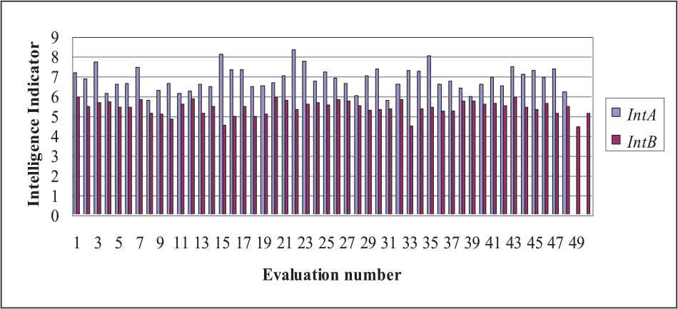
Graphical representation of IntA and IntB.
| IntA | IntB | ||||||
|---|---|---|---|---|---|---|---|
| 7.172; | 6.864; | 7.691; | 6.12; | 5.932; | 5.454; | 5.657; | 5.706; |
| 6.572; | 6.612; | 7.413; | 5.786; | 5.409; | 5.442; | 5.826; | 5.123; |
| 6.262; | 6.626; | 6.13; | 6.217; | 5.065; | 4.81; | 5.579; | 5.853; |
| 6.586; | 6.467; | 8.084; | 7.313; | 5.121; | 5.459; | 4.492; | 4.944; |
| 7.295; | 6.473; | 6.516; | 6.657; | 5.466; | 4.978; | 5.095; | 5.917; |
| 7.009; | 7.714; | 5.76; | 5.315; | 5.558; | 5.661; | ||
| 6.729; | 7.177; | 6.887; | 6.612; | 5.546; | 5.809; | 5.729; | 5.519; |
| 5.99; | 7.007; | 7.333; | 5.78; | 5.288; | 5.293; | 5.365; | 5.806; |
| 6.585; | 7.257; | 7.225; | 8.005; | 5.345; | 5.427; | 5.217; | |
| 6.592; | 6.741; | 6.37; | 5.944; | 5.244; | 5.741; | 5.724; | 5.579; |
| 6.573; | 6.911; | 6.513; | 7.447; | 5.599; | 5.506; | 5.907; | 5.421; |
| 7.066; | 7.277; | 6.924; | 7.343; | 5.312; | 5.632; | 5.101; | 5.476; |
| 6.204 | 5.111 | ||||||
IntA and IntB problem-solving intelligence evaluations results.
In Table 2, symbol “#” indicates an intelligence indicator value that is not identified as an outlier, but it is statistically further from the rest. It can be noticed that no outlier values were detected. The superscripts indices indicate at which application of the outliers' detection test those value is identified as further from the rest. It can be noticed that the outlier detection test was applied two times on IntA (at the second application it does not detect any value further from the rest), and recursively three times on IntB (at the third application it does not detect any value further from the rest). Table 2
The first two columns of Table 3, labeled as “IntA” and “IntB,” present the results of the Normality Verification and Extraction Algorithm. The CIT is calculated as the mean of intelligence indicators. SD denotes the standard deviation.
| First Application |
Second Application |
|||
|---|---|---|---|---|
| IntA | IntB | IntA* | IntB* | |
| CentrInd | 6.841 | 5.40378 | 6.81 | 5.444 |
| [LCIm, HCIm] | [6.671, 7.011] | [5.3, 5.508] | [6.648, 6.972] | [5.354, 5.535] |
| INVCentrInd | 0.1462 | 0.1851 | 0.1468 | 0.1837 |
| SD | 0.5861 | 0.3647 | 0.5515 | 0.3115 |
| Sample size | 48 | 50 | 47 | 48 |
| CV/homogeneity | 8.567/hom. | 6.749/hom. | 8.1/hom. | 5.72 CV < 10/hom. |
CV, Coefficient of Variation; SD, Standard Deviation.
Results of VerExtr algorithm.
As a first approach for the normality verification, the K–S test of normality was applied, at
| IntA | IntB | |
|---|---|---|
| K–S statistic | 0.1023 | 0.1057 |
| Pn (P-value of normality test) | >0.10 | >0.10 |
| Normality passed |
Yes | Yes |
K–S, Kolmogorov–Smirnov.
Results of K–S test applied to IntA, IntB.
Furthermore, the forthcoming processing and analysis of the Verify Evolution in Intelligence by Learning algorithm was applied. For the verification of statistical equality of standard deviations SDA and SDB, the F-test was applied. The calculation results where
The CL is established as 95%. LCIm, HCIm denotes the low and high bounds of the confidence interval of the mean.
In order to obtain a precise conclusion related to the fact that ILSBL has made an evolutionary step, as a second analysis of the normality using the Shapiro–Wilk test. By analyzing the results of the Shapiro–Wilk test for IntA and IntB presented in Table 5, can be formulated the conclusion that the data did not pass the normality assumption. For an alternative visual analysis, we created the histograms corresponding to IntA, (Figure 2) and IntB (Figure 3), and Q–Q Plots corresponding to IntA (Figure 4) and IntB (Figure 5). The provided visual representation suggests also the violation of the normality assumption.
| IntA | IntB | |
|---|---|---|
| S–W statistic | 0.977 | 0.931 |
| Pn (P-value of normality test) | 0.457 | 0.006 |
| Normality passed |
No | No |
S–W test, Shapiro–Wilk test.
Results of S–W test for IntA and IntB.
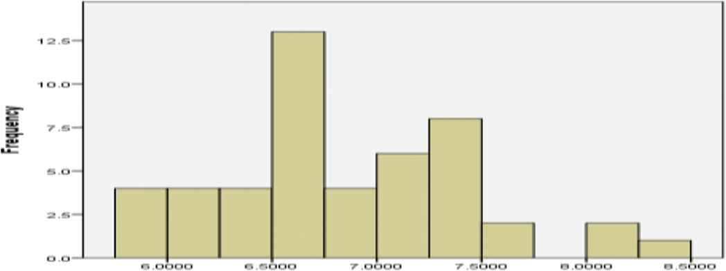
Histogram of the IntA data for the visual analysis of the normality.
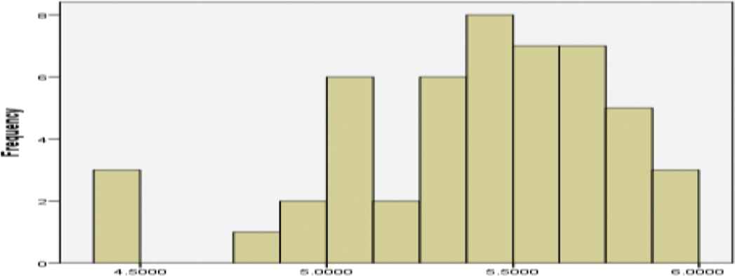
Histogram of the IntB data for the visual analysis of the normality.

Normal Quantile–Quantile (Q–Q) Plot of IntA.

Normal Quantile–Quantile (Q–Q) Plot IntB.
To obtain normally distributed data, we opted for the application of outlier intelligence detection using the Grubbs test. The decision was made also taking into consideration the expectable data normality by analyzing the drawn Q–Q plots. The Grubbs test was applied at a significance level of
In the case of IntA, at the first application of the outlier detection test, outliers were not identified, only the value 8.297 that was identified as further from the rest (calculated
| IntA* | IntB* | ||
|---|---|---|---|
| K–S statistic | 0.09878 | 0.08 | K–S test |
| Pn (calculated P-value) | >0.01 | >0.1 | |
| Normality passed |
Yes | Yes | |
| S–W statistic | 0.98 | 0.965 | S–W test |
| Pn (calculated P-value) | 0.609 | 0.161 | |
| Normality passed |
Yes | Yes |
K–S, Kolmogorov–Smirnov, S–W test, Shapiro–Wilk.
Results of normality tests applied to IntA* and IntB*.
In the case of IntB at the first application of the outlier detection test, outliers were not identified, only the value 4.405 that was identified as further from the rest (the calculated
The final obtained IntA* and IntB* passed the normality assumption according to K–S and S–W tests, thus allowing the application of the specific data analysis in order of verification if the studied system performed an evolutionary step in intelligence.
For the verification of statistical equality of standard deviations SDA* and SDB*, the F-test was applied. The obtained calculation results where
Summarizing, in the performed experimental study, first we applied the K–S test. The data passed the normality test, and based on this consideration we used the proposed metric for measuring the machine intelligence of the studied learning system. At a second approach, we applied the S–W test that is considered more powerful than the K–S test. None of IntA and IntB passed the normality assumption by using the Shapiro–Wilk test. Based on this fact it was opted for the elimination of outliers, finally obtaining normally distributed intelligence indicator data, followed by the application of the metric. The conclusion in both cases with the results presented in the previous paragraphs, was the same, that LSBL made a measurable evolutionary step in intelligence.
5. DISCUSSION
Intelligent CMASs are challenged to solve difficult practical problems in an efficient and effective way. In our study, we consider that machine intelligence measuring based on the ability of a CMAS to solve difficult problems. If learning results in a statistically significant improvement of machine intelligence then this improvement should be measurable by a metric. There are very few designed metrics that can be applied for measuring machine intelligence. Usual drawbacks of such metrics include limitations in universality, accuracy and robustness. Another important aspect that a metric should treat consists in the variability of intelligence.
Considering the previously mentioned limitations, it was proposed a novel accurate and robust metric called II-Learn (metric for measuring Intelligence Increase of artificial Learning systems) for measuring the increase of intelligence of a CMAS after a learning process.
The intelligence measuring criteria in our approach is based on some kind of difficult problem-solving ability. The fact that a specific type of problem could be solved with more or less intelligence by different CMASs is well-known. In case of a CMAS if there are some changes (changing of the problem-solving knowledge or details detained by a problem whose solving is in progress), which could be the result, for example, of performed autonomous learning, the problem-solving ability could change also (it could increases, remains unmodified or it could even decreases).
In a previous study, the MetrIntComp metric [41] with the purpose of measurement of machine intelligence of CMASs is proposed. The intelligence measuring criteria was also based on the principle of difficult problem-solving ability. MetrIntComp was designed to be robust, which is based on the fact that in the process of classification it uses the Two-Sample Unpaired Mann–Whitney test that is known as a non-parametric robust test [116]. Since both metrics quantify the problem-solving intelligence of learning systems, both II-Learn and MetrIntComp can be considered comparable.
The novelty of II-Learn versus MetrIntComp is based on different performed processing and analyses. One of the significant differences from the performed computations point of view between the two metrics is that II-Learn uses Two-Sample Unpaired T-test [88–90] and Welch Two-Sample Unpaired T-test (Welch's test) [91,92] for intelligence comparison as the parametric analog of the Mann–Whitney test. Two-Sample Unpaired T-test is appropriate in the case of equality from the statistical point of view between the SDs of the two intelligence indicators samples. One representing the problem-solving intelligence evaluation result of the system before learning, the other one representing the problem-solving intelligence evaluation result after the learning. The Welch's test [90] is more appropriate when the SDs are not equal from the statistical point of view. Welch's test represents a generalization of the Two-Sample Unpaired T-test, in the sense that it can be used in case of unequal SDs [91]. In [92] the Welch's test was proved more reliable than Two-Sample Unpaired T-test when the two samples have unequal SDs and unequal sample sizes. The statistical power of Welch's t-test is very close to that of Two-Sample Unpaired T-test, when the population SDs are equal and sample sizes are balanced [92]. In [117] a generalization to the Welch's t-test was presented, in order to be applied to any number of samples (even more than two samples). That study showed that this generalization is more robust than One-Way Analysis of Variance (ANOVA) that can be applied to any number of samples; however, it requires the assumption of normality and equality of sample sizes.
The main advantage of II-Learn over the MetrIntComp is its accuracy for smaller sample sizes. It takes into consideration the sample intelligence indicator data property to be normally distributed. Based on this fact, a mathematically grounded calculus is applied for verification if the studied CMAS made an evolutionary step, which is the most appropriate for normally distributed data. In the case of non-Gaussian intelligence indicator data, a transformation should be applied (see Table 1), resulting in enhanced robustness. Another advantage in the calculation of II-Learn over MetrIntComp is that it considers the presence of possible extremes and applies a methodology to remove them from the samples.
Similarly to the humans, intelligent computing systems have a variability of intelligence in problem-solving. The elaborated II-Learn metric takes into consideration this variability in problem-solving intelligence. In a specific situation, the studied system's reaction could be more or less intelligent. As a measure of the CIT, we established as the most representative the mean based on the consideration that the data were sampled from a Gaussian population.
The Central Limit Theorem can be enounced as follows [118]: given independent random samples of M observations, the distribution of sample means approaches normality as the size of M increases, regardless of the shape of the population distribution. In general, many studies consider that M should be at least 30 or higher. In [119] it is proved that in the case of samples consisting of hundreds of data, the distribution of the data can be ignored. In our case study making hundreds of problem-solving intelligence, evaluations could be very expensive or even impossible. As a good practice, we recommend using intelligence indicators sets larger than 30. Thus, we suggest the application of II-Learn metric with at least 30 experimental evaluation of the learning system before the learning process and with at least 30 experimental evaluations after the learning process.
The number of necessary experimental evaluations is also an important issue that should be analyzed in order to formulate scientifically correct conclusions. Conclusions formulated based on too few experimental evaluations could be inaccurate or even incorrect. Sometimes the realization of an experiment could be expensive or time-consuming, thus suggesting the limitation of the number of experiments. Based on this aspect we consider that, in some cases, a compromise must be made with respect to the number of experiments that will be realized, and the chance of an error occurrence (in our approach the probability of occurrence of a type I error or a type II error). In this paper, we proposed a calculus for the exact estimation of the number of experimental evaluations.
Different metrics presented in the literature like those based on analytical models are limited in universality. II-Learn metric is universal, it can be used for intelligent learning systems generally; it does not depend on aspects like the intelligent system's architecture. II-Learn can be applied even in the case of individual learning agents. The universality is assured based on our specific approach on that a system's intelligence is evaluated on some difficult problems-solving evaluations before a learning process and problem-solving intelligence evaluations after a learning process. On these two obtained intelligence indicators data sets is applied some specific calculus in order to verify if the intelligence as result of learning is changed, and if this has as an effect that the system has made an evolutionary or involutionary step in intelligence. The method of the metric provides both accuracy and robustness, addressing the variability in problem-solving intelligence.
We would like to mention that the significance that we give to the notion universality is different from the significance given to universality in some other studies, like that presented by Hernandez-Orallo and Dowe [60]. The researchers proposed the idea of universal anytime intelligence test able to measure any kind of natural/biological and AI. In our approach, the notion of universality in intelligence measuring is considered independent of the studied system architecture. We do not intend to build metrics able to measure both biological (including the human) and AI.
6. CONCLUSIONS
In this paper, we proposed a novel metric called II-Learn, for measuring a cooperative multiagent system (able to learn) intelligence, and the verification if the learning resulted in an intelligence level/measure modification by statistically significant increasing or decreasing. II-Learn metric takes into consideration the variability in the problem-solving intelligence (lower and higher intelligence in different situations). Advantages of the II-Learn metric consist in universality, accuracy and robustness.
The proposed II-Learn metric was compared with the state-of-the-art MetrIntComp metric that was also designed to be robust. For the II-Learn metric robustness increase we proposed solutions based on the experimental intelligence evaluations results transformation and detection of experimentally obtained outlier intelligence values. The main advantage of II-Learn over the MetrIntComp is its increased accuracy. Another advantage of II-Learn over MetrIntComp is that it considers the presence of possible outliers and applies a methodology to remove them from the measured problem-solving intelligence samples.
For proving the effectiveness of the metric, we performed a case study, which showed that the learning process had as an effect the making of an evolutionary step in the intelligence (the studied system evolved).
II-Learn is an original metric, and it will represent the basis for the intelligence measurement of learning systems, and intelligence increase based on learning, in many future researches related to different intelligent systems, which operate individually or cooperate with each other. Examples of practical applications, may include intelligent robotic transportation systems; swarm of robots performing different tasks in different environments; agents specialized in solving different tasks in the healthcare, agents and cooperative multiagent systems able to solve different tasks in transportation.
CONFLICT OF INTEREST
No conflict of Interest.
AUTHORS' CONTRIBUTIONS
All the authors contributed equally to this work.
ACKNOWLEDGMENTS
This work was supported by the project CNFIS-FDI-2019-0453: Support actions for excellence in research, innovation and technological transfer at “Vasile Alecsandri” University of Bacău (ACTIS-Bacău), financed by the National Council for Higher Education, Romania.
REFERENCES
Cite this article
TY  - JOUR
AU  - László Barna Iantovics
AU  - Dimitris K. Iakovidis
AU  - Elena Nechita
PY  - 2019
DA  - 2019/11/14
TI  - II-Learn—A Novel Metric for Measuring the Intelligence Increase and Evolution of Artificial Learning Systems
JO  - International Journal of Computational Intelligence Systems
SP  - 1323
EP  - 1338
VL  - 12
IS  - 2
SN  - 1875-6883
UR  - https://doi.org/10.2991/ijcis.d.191101.001
DO  - 10.2991/ijcis.d.191101.001
ID  - Iantovics2019
ER  -