
Subgroup Discovery on Multiple Instance Data
- DOI
- 10.2991/ijcis.d.191213.001How to use a DOI?
- Keywords
- Supervised descriptive patterns; Subgroup discovery; Multi-instance data; Metaheuristics
- Abstract
To date, the subgroup discovery (SD) task has been considered in problems where a target variable is unequivocally described by a set of features, also known as instance. Nowadays, however, with the increasing interest in data storage, new data structures are being provided such as the multiple instance data in which a target variable value is ambiguously defined by a set of instances. Most of the proposals related to multiple instance data are based on predictive tasks and no supervised descriptive analysis can be provided when data is organized in this way. At this point, the aim of this work is to extend the SD task to cope with this type of data. SD is a really interesting task that aims at discovering interesting relationships between different features with respect to a specific target variable that is of interest for the user or the problem under study. In this regard, this paper presents three different approaches for mining interesting subgroups in multiple instance problems. The proposed models represent three different ways of tackling the problem and they are based on three well-known algorithms in the SD field: SD-Map (exhaustive search approach), CGBA-SD (Comprehensible Grammar-Based Algorithm for Subgroup Discovery) and NMEEF-SD (multi-objective evolutionary fuzzy system). The proposals have been tested on a wide set of datasets, including 10 real-world and 20 synthetic datasets, aiming at describing how the three methodologies behave on different scenarios. Any comparison is unfair since they are completely different methodologies.
- Copyright
- © 2019 The Authors. Published by Atlantis Press SARL.
- Open Access
- This is an open access article distributed under the CC BY-NC 4.0 license (http://creativecommons.org/licenses/by-nc/4.0/).
1. INTRODUCTION
Data mining, which is defined as the process of discovering useful information usually hidden in data, is generally divided into two main tasks: predictive and descriptive. The former includes techniques that predict a target variable (object or event) by an instance represented as a vector of features. Descriptive tasks, on the contrary, do not consider any target variable and they aim at finding useful insights (generally in terms of co-occurrences) from the set of features [1]. Until recently, these techniques have been researched by two different communities: predictive tasks principally by the machine learning community, and descriptive tasks mainly by the data mining community. In some specific fields, however, it is required that both tasks converge at some point, which has given rise to the concept of supervised descriptive pattern mining [2]. The main aim now is to understand an underlying phenomena (according to a target variable) and not to classify new examples. Among existing techniques for mining supervised descriptive patterns, subgroup discovery [3] (SD) is, by large, the most well-known. It aims at identifying a set of features (patterns) of interest according to their distributional unusualness with respect to a certain property of interest (target variable). In other words, SD describes data subsets for a given target variable by means of independent and simple rules unlike predictive learning that explains future behavior through complex models.
SD has been used in a wide range of problems [2] in which the target variable is unequivocally defined by an instance, that is, a vector of features. In some other problems, however, data is organized as a bag of instances all somehow related (e.g., because all are due to the same hidden cause or factor) and there is a target variable for each bag of instances and not for each single instance [4]. As a matter of clarification, let us consider data gathered from a supermarket in which we want to obtain insights that describe customers' purchasing habits based on the type of customers (target variable). There may be occasional and common customers and their number of transactions (instances) is therefore dissimilar. Describing data subsets for a given target variable (the type of customer) by means of independent and simple rules that denote some distributional unusualness on that problem cannot be performed by a traditional SD task. Instead, SD is required to be analyzed as a multiple-instance (MI) problem where the aim is to learn from a set of feature vectors where each of these sets has an associated outcome or target variable.
The MI problem [5] has been generally associated with predictive tasks, which is known as multiple instance learning (MIL). MIL has been widely studied and there exist a taxonomy of MIL methods [6]. First, instance-based methods are based on instance-level information in the sense that the learning process considers the characteristics of individual instances without looking at more global characteristics of the whole bag. Second, bag-based methods take into account the global bag-level information since the discriminative decision is taken by looking at the whole bag instead of aggregating local instance-level decisions. Finally, embedded methods consider each bag to be mapped to a single feature vector which summarizes the relevant information about the whole bag. In some recent studies, however, it was demonstrated that the MI problem is not a matter of predictive tasks but it is also of high interest for descriptive analyses. In a descriptive task there is no target variable associated and instances within a bag are related due to a specific factor, for example, multiple purchases of the same customer in a market basket analysis. In such descriptive analysis, the MI problem cannot be addressed neither through bag-based nor embedded methods. Instead, instances are important in isolation and should be analyzed one by one for each bag.
Taking all these points into account and considering the importance of MI problems, the aim of this paper is to extend the SD problem to cope with MI data. In this regard, this paper presents three different SD approaches for mining interesting subgroups in MI problems. The proposed models are based on three well-known algorithms in the SD field and following completely different methodologies:
The paper is structured as follows: Section 2 includes some formal definitions for SD and MIL. Additionally, this section includes the contribution of this work. Section 3 describes the three proposals. Section 4 describes the datasets used in the experimental stage, the algorithms' set-up and a discussion of the obtained results. Finally, in Section 5, some concluding remarks are outlined.
2. PRELIMINARIES
In this section the most important concepts as well as formal definitions related to SD and MI learning are provided. Finally, the key points about the contribution of this work are outlined.
2.1. Subgroup Discovery
SD is a descriptive data mining technique grouped into the SDSR (Supervised Descriptive Rule Discovery) concept [12], which also includes other interesting tasks [2] such as contrast set mining and emerging pattern mining. The idea of SD was introduced by Kloesgen [13] and Wrobel [14], and it was formally defined by authors as:
In subgroup discovery, we assume we are given a so-called population of individuals (objects, customers, etc.) and a property of those individuals we are interested in. The task of subgroup discovery is then to discover the subgroups of the population that are statistically “most interesting”, i.e., they are as large as possible and have the most unusual statistical (distributional) characteristics with respect to the property of interest.
The aim of SD is the search for relations between different properties or variables of a set with respect to a target variable [15]. In SD, the ultimate aim is to describe and understand the underlying phenomena with respect to an interest property. An illustrative example allows to understand it easily:
A medical center wants to know in what circumstances a patient may suffer a type of cancer, the intention is not to predict cancer, but to describe the risk factors that lead to this.
The representation of the knowledge plays an important role to correctly describe the phenomena under study, and this descriptive analysis is carried out by individual rules that denote relations between variables, that is, rules [1] in the form:
SD uses descriptive induction through supervised learning which is widely used in classification. However, SD is differentiated with respect to classification techniques because it attempts to describe knowledge by data while a classifier attempts to predict the target value for new data to incorporate in the model. Furthermore, SD does not obtain a precise and complex model which perfectly divides the space into a determined regions. Instead, a SD algorithm obtains sets of independent rules that describe each value of the target variable and should satisfy the following properties [16]:
Interpretable. The number of rules and the complexity of these rules (with respect to the number of variables) must be easily interpretable by experts, that is, a low number of rules with few variables is desirable.
Novelty. Rules must be statistically interesting so they should describe an unusual statistical distribution with respect to the
Trade-off generality-precision. SD is required to obtain results with a good precision (where the majority examples covered by the rule belong to the specific target variable) and covering the major number of examples.
A key element in the SD task is the right choice of measures that quantify the importance of the extracted knowledge. A wide set of quality measures has been proposed in literature and there is no current consensus about which are the most suitable ones. Considering the three main properties previously presented, the most appropriate quality measures are the following:
Number of rules obtained for the model. Any SD approach must obtain a set of simple and interpretable rules for the problem under study. In many situations, though, the obtained subgroups are not interesting at all so not all the values of the target variable are covered.
Number of variables. It is measured as the number of conditions within the rule. The number of variables for a set of rules is computed as the average number of the variables for each rule of that set.
Unusualness is the weighted relative accuracy of a rule [17] which measures interest and a trade-off between generality and precision. It is computed as:
Unusualness can be described as the balance between the coverage of the rule and its accuracy gain, where
Sensitivity is the proportion of actual matches that have been correctly classified [13] and it has a component based on generality. This quality measures can be found in the literature as the Support based on the examples of the class, Recall or
Confidence determines how reliable the rule is, that is, it quantifies the relative frequency of examples satisfying the complete rule among those satisfying only the antecedent [19]. This quality measure takes values in the range
The applicability of SD to real-world problems can be observed throughout the literature widely. For example, in [20,21] descriptions in bioinformatic domains are performed, in medicine [22], in industry [23], or e-learning [24] among others [25].
2.2. Multiple Instance Learning
In traditional supervised learning each object to be learned is unequivocally described by a feature vector that is associated to an outcome or target variable (see Figure 1(a)). In MIL [5], however, the data structure is more complex and each object or target variable is ambiguously defined by an undetermined number of feature vectors (multiple instances in the MIL jargon) that are related due to the same hidden cause (see Figure 1(b)). According to a recent review [6], each bag (set of instances) has an associated target variable value, but we do not know the target variable values of the individual instances that conform the bag. In its formal definition, let us assume a dataset
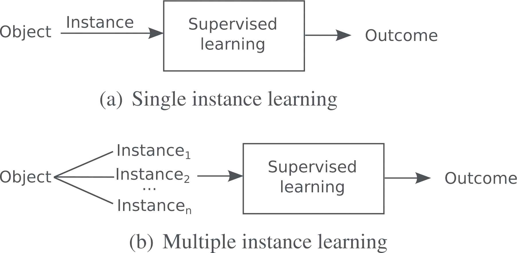
Predictive task where each object is: (a) unequivocally described by a feature vector; (b) ambiguously described by an undetermined number of feature vectors.
In a recent overview [6], existing MIL methods were grouped into a small set of compact paradigms (instance-space, bag-space and embedded-space) according to how they manage the information from the MI data. Beginning with the instance-space paradigm, the discriminative information is considered to lie at the instance-level (only characteristics of individual instances are considered) so a discriminative instance-level classifier is trained to separate the instances in positive bags from those in negative ones. Thus, once a new bag is obtained, it is classified according to the aggregation of instance-level scores. The instance-space paradigm considers two different methods, that is, the ones following the standard MI assumption and the ones following the collective assumption. The standard MI assumption, stated by Dietterich et al. [26], defines a positive result if and only if at least one of the instances within a bag produces a positive result. On the contrary, a negative result is provided if all the instances within a bag produce a negative result. As for the collective assumption, Weidmann et al. [27] determined a bag as positive if and only if at least a certain number of instances in such bag produce a positive outcome. This assumption is known as the threshold-based MIL assumption. An additional assumption (count-based assumption) was also defined by considering a minimum and a maximum number of instances required to be positive in order to consider the bag as positive.
Focusing on the bag-space paradigm [6], the discriminative information is considered to lie at the bag-level. In this paradigm each bag is treated as a whole entity, and the learning process discriminates between entire bags. It is considered that this paradigm is based on bag-level information since the discriminative decision is taken by looking at the whole bag. In this regard, some methods have defined a distance function to compare two bags and used such distance function in a distance-based classifier such as K-NN or SVM. Finally, the third type of paradigm defined in [6] is related to an embedded-space is also based on extracting global information about the bag. To do that, each bag is associated to a feature vector that summarizes the characteristics of the whole bag. Thus, the two last paradigms (bag-space and embedded-space) are based on extracting global information about the bags. The main difference among them is based on the way bags are measured to be compared, that is, implicitly through a distance function (bag-space) or explicitly through a summarized feature vector (embedded-space).
2.3. Contribution
SD has been used in a wide range of problems in which the target variable is unequivocally defined by an instance, that is, a vector of features. Nowadays, with the increasing interest in data storage, data is organized in multiple forms and one of the most well-known is in bags of instances that are somehow related due to the same hidden (or known) cause. In this data representation, called MI data, a target variable is associated to each bag of instances and not to each single instance. This type of data has been generally considered through predictive tasks in which the target variable associated to each bag (set of instances) is predicted. This data representation, however, has not been considered from a descriptive point of view which is also of high interest due to its ability to provide useful and unusual features associated to each target variable value through independent and simple rules.
Taking into account the importance of MI problems, the aim of this paper is to extend the SD problem to cope with MI data. In this regard, this paper presents different SD approaches for mining and describing interesting subgroups in MI problems. The approaches are based on three well-known SD algorithms considering different methodologies. Thus, we have considered the most well-known exhaustive search SD approach, that is, the SD-Map algorithm based on a really efficient pattern mining algorithm such as FP-Growth. Two additional SD approaches based on non-exhaustive search methodologies are also considered. One is based on multi-objective evolutionary fuzzy systems, that is, NMEEF-SD, whereas CGBA-SD, the other one, is based on grammar-guided genetic programming. Finally, it is important to remark that the MI problem was addressed by considering the instance-space paradigm since the other two paradigms transform the MI problem into a single instance one and, therefore, it is not useful from a descriptive point of view.
3. PROPOSALS
Most of the existing algorithms for SD are focused on binary or nominal target attributes, for which heuristic [28] as well as exhaustive search methods [3] are applied. Focusing on heuristic approaches, the way in which these approaches deal with features that are defined in a continuous domain has been of great interest for many researchers. In this regard, different fuzzy systems have been proposed for the SD problem from which NMEEF-SD has been demonstrated to be the most promising one according to the statistical analysis carried out in [10]. Additionally, the use of grammars to encode solutions on continuous domains to provide expressive and flexible solutions has also been considered for the SD problem. In this sense, the CGBA-SD algorithm has been proved to perform statistically better than the existing algorithms as it is demonstrated in [9]. It should highlight that most heuristic approaches are often preferable due to exhaustive search methods take long time to explore the complete search space in certain domains. The use of evolutionary algorithms for SD is very well suited because these algorithms perform a global search in the space as it is demonstrated [28]. However, due to efficient pruning techniques, many exhaustive search approaches can achieve sufficiently good runtimes even in complex domains. In this sense, SD-Map [7] is the most well-known exhaustive search algorithm for SD since it is a really promising option for efficiently mining large datasets.
According to the aforementioned description, three promising algorithms (SD-Map, CGBA-SD and NMEEF-SD) that follow different methodologies in the SD field have been taken as baseline. These three approaches have been accordingly adapted to the MI problem by considering the instance-space paradigm, which is the one that best fits to the SD problem, as follows:
SD-Map-MI is based on the SD-Map algorithm [7], an exhaustive search algorithm that uses the well-known FP-Growth method [8] adapted for the SD task. It is important to highlight that this method can not work with numeric variables, so it makes necessary a previous discretization phase. The algorithm performs a first scan of the dataset in order to prune those features with a support lower than a threshold. Then, it sorts the features according to the support in order to put features with higher values closer to the root. After that, the algorithm performs a depth-first search where the subgroups are evaluated directly, without referring to other intermediate results. After the processing of the subgroups, the algorithm can obtain the best
The main motivation for considering this algorithm is the capability to extract any feasible solution since it is an exhaustive search approach. Additionally, SD-Map is based on FP-Growth that is one of the most promising, in terms of runtime, algorithms for mining frequent patterns. Thus, SD-Map not only is able to extract any feasible solution in data but it also achieves an incredibly good performance. In general terms, the main advantage of using SD-Map is that it analyzes the whole search space and, therefore, the obtained solutions are really the best ones. Nevertheless, two main downsides should be taken into account when using SD-Map. First, it only copes with discrete values so data defined in a continuous domain needs to be discretized beforehand, assuming a loss of information. Second, it requires large amount of memory when extremely large datasets are analyzed so real-world datasets are hardly analyzed (a search space restriction is required).
CGBA-SD-MI based on the CGBA-SD algorithm [9] which is an evolutionary algorithm that uses a genetic programming approach [28] combined with the use of a context-free grammar in order to obtain comprehensive rules. The use of grammars provides expressibility, flexibility and the ability to restrict the search space. CGBA-SD is within the “chromosome = rule” approach where an individual is represented by means of a tree structure which can represent nominal variables and continuous ones by means of random intervals, which are optimized in a post-processing phase. The algorithm uses an initialization procedure where individuals generated have a fitness over zero always. The fitness function is the product of the support and confidence of the individual. The genetic operators used can automatically change their probability of application depending on whether is necessary more diversity or not. The final population keeps those individuals with a confidence greater than a threshold and equivalence between individuals. The adaptation to the MI problem has been performed on the evaluation phase, where the count of the features that form an individual is calculated. Here, the standard assumption is considered, that is, the counts of the features are increased only once per bag, for example, if a feature
The main motivation for considering this algorithm is its capability to extract solutions in any domain (continuous and discrete) and with an almost constant runtime. This algorithm [9] was already compared to multiple SD algorithms obtaining the best results, specially when considering evolutionary computation solutions. In general terms, the main advantage of using CGBA-SD is its ability to cope with data defined in continuous domains so no discretization step is required. Another important advantage of CGBA-SD is the use of a context-free grammar to encode solutions so the end user is able to describe beforehand the shape of the solutions to be obtained. Nevertheless, the main drawback of this algorithm is its inability to analyze the whole search space and, therefore, some promising solutions might be skipped.
NMEEF-SD-MI is based on the NMEEF-SD [10] which is an evolutionary fuzzy system based on a multi-objective algorithm called NSGA-II [11]. This algorithm encodes the solutions according to the “chromosome = rule” approach, where only the antecedent is represented in the chromosome and the consequent is prefixed to one of the possible values of the target variable in the evolution. In this way the algorithm is executed as many times as the number of values for the target variable it contains. The algorithm employs different genetic operators in order to promote generality and diversity within the population and to obtain interesting subgroups for the SD technique. It is very important to highlight the use of the multi-objective approach because it allows the experts the possibility to use different quality measures as objectives. In this way the final Pareto front obtained by NMEEF-SD is the set of non-dominated solutions with respect to the quality measures considered. As can be observed in [10] the best results for this algorithm are obtained with the use of the quality measures unusualness and sensitivity. Finally, a screening function is performed at the end of the evolutionary process in order to return only those solutions which reach a pre-determined confidence threshold. The adaptation of this algorithm to the MI problem is, similarly to the other three approaches, based on the standard assumption in order to calculate the quality measures with respect to bags. Again, a bag is considered as covered by an individual if at least one of its instances is covered by the individual.
The main motivation for considering this algorithm is the possibility of addressing the SD problem by means of a multi-objective evolutionary fuzzy system such as NMEEF-SD, which is one of the most well-known algorithms in the SD literature. The main advantage of this algorithm is its ability to provide the experts with the possibility to use different quality measures as objectives, in such a way that final solutions are those included in the set of non-dominated solutions with respect to the considered quality measures. Additionally, NMEEF-SD-MIL is able to obtain a diverse and interesting set of rules without requiring a pre-processing step of transforming continuous features into discrete ones. Finally, a major drawback of this algorithm is its inability to analyze the whole search space and, therefore, some promising solutions might be skipped.
According to the SD definition, the main objective is to describe the underlying phenomena of a problem. Thus, the goal is to know why a positive (or a specific target value for non-binary problems) match is produced. In this sense, the match may be produced according to any of the defined assumptions. However, since many different domains are considered here and the standard assumption has been widely used on different scenarios, this very assumption has been pre-defined. The final aim is to easily describe the underlying phenomena with simple and interpretable rules that covers the major number of bags. A trade-off between generality-precision and novelty is achieved by the use of quality measures, such as unusualness, sensitivity or confidence, on the mining phase as a constraint in order to prune non-interesting rules.
4. EMPIRICAL STUDY
In this experimental study, we first describe the datasets considered in this experimental stage, including either widely-known MIL benchmarks and synthetic datasets. Finally, the results obtained by each of the proposed algorithms are outlined. It should be highlighted that the intention of this experimental analysis is not to compare the results of the algorithms for specific data but to provide an overview on the usefulness of this new problem formulation by considering three different methodologies.
4.1. Experimental Setting
In this subsection, the application domains and the parameters' settings used in the algorithms are described.
4.1.1. Dataset domains
Two different studies have been performed in this contribution:
Firstly, a varied set of 10 benchmarks that represent different real-world applications in MIL are employed. For example, drug activity consists of determining whether a drug molecule will bind strongly to a target protein, whereas content-based image retrieval aims at identifying target objects in images. Detailed information about these problems can be observed in Table 1.
Secondly, 20 artificial datasets have been generated in order to obtain a generalized study and to improve the analysis of this study. These datasets include different properties (summarized in Table 2) regarding the number of features, instances, bags and instances per bags. In the generation of these datasets different features have been considered: minimum and maximum number of instances per bag; number of attributes; and number of bags. Moreover, it is important to remark that all the attributes or features are defined in continuous domain, taking random values within the ranges [1, 5], [1, 10] and [1, 100].
| Dataset | Bags | Attributes | Instances | Average Bag Size |
|---|---|---|---|---|
| EastWest [29] | 20 | 24 | 213 | 10.65 |
| Elephant [30] | 200 | 233 | 1391 | 6.96 |
| Fox [30] | 200 | 233 | 1320 | 6.60 |
| Musk1 [26] | 92 | 166 | 476 | 5.17 |
| Musk2 [26] | 102 | 166 | 6598 | 64.69 |
| Mutagenesis-Atoms [31] | 188 | 10 | 1618 | 8.61 |
| Mutagenesis-Bonds [31] | 188 | 16 | 3995 | 21.25 |
| Mutagenesis-Chains [31] | 188 | 24 | 5349 | 28.45 |
| Tiger [30] | 200 | 233 | 1220 | 6.10 |
| WestEast [29] | 20 | 24 | 213 | 10.65 |
Information about benchmarks.
| Dataset | Bags | Attributes | Instances Per Bag | Dataset | Bags | Attributes | Instances Per Bag |
|---|---|---|---|---|---|---|---|
| ds-01 | 400 | 10 | [1, 8] | ds-02 | 450 | 10 | [1, 8] |
| ds-03 | 500 | 10 | [1, 8] | ds-04 | 500 | 6 | [1, 4] |
| ds-05 | 450 | 6 | [1, 4] | ds-06 | 400 | 6 | [1, 4] |
| ds-07 | 3000 | 8 | [1, 5] | ds-08 | 4000 | 7 | [1, 5] |
| ds-09 | 5000 | 4 | [1, 5] | ds-10 | 3500 | 9 | [1, 10] |
| ds-11 | 4500 | 5 | [1, 10] | ds-12 | 150 | 20 | [1, 3] |
| ds-13 | 150 | 40 | [1, 3] | ds-14 | 200 | 15 | [1, 3] |
| ds-15 | 400 | 35 | [1, 3] | ds-16 | 30 | 10 | [1, 5] |
| ds-17 | 50 | 8 | [1, 5] | ds-18 | 70 | 6 | [1, 5] |
| ds-19 | 90 | 10 | [1, 5] | ds-20 | 100 | 4 | [1, 5] |
General information about the artificial datasets.
All the datasets used in this study were partitioned using a 10-fold stratified cross validation, which avoids the arbitrariness and the dependence of the results with respect to the classical partitioning. All the partitions obtained for each dataset are publicly available at http://simidat.ujaen.es/papers/SD-MIL, so future comparisons can be easily performed. Finally, it should be remarked that both benchmark and artificial datasets are composed by continuous features. In this regard, due to some algorithms like SD-MAP cannot work on this type of datasets, a pre-processing discretization has been carried out. Two different approaches (Fayyad [32] and Uniform Frequency [33] in ten intervals) has been performed, and the quality with respect to the best configuration was measured.
4.1.2. Set-up of the algorithms
The parameters used for the new SD proposals for MI are summarized in Table 3. These parameters have been selected with respect to the recommendations performed by the authors in their original works. Additionally, the stochastic algorithms were run ten executions for each partition, that is, an average value is obtained from 100 values (10 partitions × 10 times) for each dataset. The values of number of rules, number of variables, unusualness, sensitivity and confidence are computed as the average for all rules. It should be highlighted again that SD-Map-MI and CGBA-SD-MI use a crisp confidence whereas the NMEEF-SD-MI employs the fuzzy confidence. Both crisp confidence and fuzzy confidence are equivalent so the same acronym was considered.
| Algorithm | Parameters |
|---|---|
| SD-Map-MI | Minimum support = 0.1; Subgroup return = 3; Subgroup for each class = True; Number maximum of selectors = 3; Quality function = Unusualness |
| CGBA-SD-MI | Minimum confidence = 0.7; Population size = 50; Number of generations = 100 |
| NMEEF-SD-MI | Objective1 = Sensitivity; Objective2 = Unusualness; Linguistic labels = (3, 5 and 7); Minimum confidence = (0.6, 0.7, 0.8 and 0.9); Population size = 50; Maximum evaluations = 10000; Crossover probability = 0.60; Mutation probability = 0.10 |
Notes. MI = multiple instance; SD = subgroup discovery.
Parameters of the algorithms.
4.2. Results and Discussion
In this subsection, the results obtained for each algorithm and a complete analysis about these results are presented. It is important to note that the complete results for each algorithm are publicly available at http://simidat.ujaen.es/papers/SD-MIL. Finally, it is required to remark that the experimental study presented in this contribution aims to show the validity of SD through different approaches and MI problems, providing a good possibility to find out new knowledge which could be interesting for the experts.
4.2.1. SD-Map-MI
Results obtained for the SD-Map-MI algorithm at the first and second group of datasets are presented in Tables 4 and 5, respectively. In a general way, SD-Map-MI has a poor behavior as can be observed in the results obtained where results are not interesting because they have a low quality and bad trade-off between sensitivity and confidence. This problematic is related to the loss of information for the previous discretization process applied into the datasets (remember that this algorithm is unable to work with continuous data). Finally, it is also remarkable the large number of rules per target variable value that SD-Map-MI obtains. In some datasets, for example, EastWeast, SD-Map-MI is unable to extract any subgroup due to there is no subgroup that satisfies the pre-defined parameters (see Table 3) and the loss of information of the discretization process.
| Dataset | Number of Rules | Number of Variables | Unusualness | Sensitivity | Confidence |
|---|---|---|---|---|---|
| EastWest | 0.00 | 0.00 | 0.000 | 0.000 | 0.000 |
| Elephant | 6.00 | 3.00 | 0.400 | 0.050 | 0.250 |
| Fox | 6.00 | 2.50 | 0.325 | 0.100 | 0.257 |
| Musk1 | 6.00 | 2.33 | 0.338 | 0.192 | 0.417 |
| Musk2 | 6.00 | 2.67 | 0.500 | 0.139 | 0.500 |
| Mutagenesis-atoms | 6.00 | 2.67 | 0.164 | 0.000 | 0.000 |
| Mutagenesis-bonds | 6.00 | 2.83 | 0.321 | 0.000 | 0.000 |
| Mutagenesis-chains | 3.00 | 3.00 | 0.222 | 0.000 | 0.000 |
| Tiger | 6.00 | 3.00 | 0.267 | 0.117 | 0.140 |
| WestEast | 0.00 | 0.00 | 0.000 | 0.000 | 0.000 |
| AVERAGE | 4.50 | 2.20 | 0.254 | 0.060 | 0.156 |
Notes. MI = multiple instance; SD = subgroup discovery.
Results obtained for the benchmarks by considering the SD-Map-MI algorithm.
| Dataset | Number of Rules | Number of Variables | Unusualness | Sensitivity | Confidence |
|---|---|---|---|---|---|
| ds01 | 6.00 | 1.00 | 0.263 | 0.075 | 0.127 |
| ds02 | 4.00 | 1.50 | 0.342 | 0.207 | 0.280 |
| ds03 | 4.00 | 1.50 | 0.280 | 0.140 | 0.200 |
| ds04 | 6.00 | 1.83 | 0.493 | 0.327 | 0.499 |
| ds05 | 6.00 | 1.83 | 0.446 | 0.355 | 0.437 |
| ds06 | 6.00 | 1.00 | 0.421 | 0.142 | 0.362 |
| ds07 | 6.00 | 1.83 | 0.383 | 0.332 | 0.375 |
| ds08 | 6.00 | 1.00 | 0.369 | 0.125 | 0.246 |
| ds09 | 6.00 | 1.00 | 0.386 | 0.155 | 0.288 |
| ds10 | 6.00 | 1.00 | 0.223 | 0.124 | 0.155 |
| ds11 | 3.00 | 1.66 | 0.344 | 0.342 | 0.344 |
| ds12 | 6.00 | 1.67 | 0.500 | 0.563 | 0.513 |
| ds13 | 6.00 | 1.67 | 0.719 | 0.813 | 0.710 |
| ds14 | 6.00 | 1.67 | 0.475 | 0.450 | 0.460 |
| ds15 | 6.00 | 1.67 | 0.638 | 0.550 | 0.656 |
| ds16 | 6.00 | 1.00 | 0.125 | 0.083 | 0.083 |
| ds17 | 6.00 | 1.00 | 0.222 | 0.167 | 0.181 |
| ds18 | 6.00 | 1.00 | 0.250 | 0.083 | 0.250 |
| ds19 | 6.00 | 1.00 | 0.367 | 0.133 | 0.306 |
| ds20 | 6.00 | 1.00 | 0.333 | 0.133 | 0.178 |
| AVERAGE | 5.65 | 1.34 | 0.379 | 0.265 | 0.332 |
Notes. MI = multiple instance; SD = subgroup discovery.
Results obtained in the artificial datasets by considering the SD-Map-MI algorithm.
4.2.2. CGBA-SD-MI
Tables 6 and 7 present the results obtained by CGBA-SD-MI for the benchmark and artificial datasets, respectively. CGBA-SD-MI has a good homogeneity in the study of the benchmarks as can be observed in the average values obtained with good values of unusualness and an excellent trade-off between sensitivity and confidence. In general, the algorithm extracts precise rules with values higher than 60% in sensitivity, denoting that the majority examples for the value of the target variable analyzed are covered. On the other hand, the interpretability of this model is highlighted with respect to the number of rules and variables extracted because it obtains a low number of rules with few variables in the antecedent which would allow to the expert an easy analysis of the problems. With respect to the results obtained in the artificial datasets by CGBA-SD-MI, similar conclusions as in the previous study can be achieved. It obtains a good trade-off between sensitivity and confidence with high values in both quality measures. In unusualness the algorithm also gets goods values, so the behavior of CGBA-SD-MI is very homogeneous in the complete study. Moreover, it obtains one rule for each value of the target variable with a low number of variables, that is, all values for the target variable are represented and rules are always between one and two variables instead of we have even analyzd datasets with 40 variables. In this way, the algorithm has a good interpretability. Finally, some examples of rules extracted by CGBA-SD-MI on different real-world datasets can be observed in Table 8. As shown, this algorithm is able to obtain rules for each target value, and the rules obtained includes few variables and, therefore, are really understandable for a user.
| Dataset | Number of Rules | Number of Variables | Unusualness | Sensitivity | Confidence |
|---|---|---|---|---|---|
| EastWest | 2.00 | 2.00 | 0.575 | 1.000 | 0.575 |
| Elephant | 2.00 | 1.18 | 0.648 | 0.576 | 0.671 |
| Fox | 2.24 | 1.20 | 0.564 | 0.247 | 0.564 |
| Musk1 | 2.10 | 1.47 | 0.689 | 0.718 | 0.683 |
| Musk2 | 2.08 | 1.54 | 0.639 | 0.573 | 0.647 |
| Mutagenesis-Atoms | 2.02 | 1.10 | 0.582 | 0.600 | 0.671 |
| Mutagenesis-Bonds | 2.00 | 1.18 | 0.596 | 0.611 | 0.646 |
| Mutagenesis-Chains | 2.06 | 1.22 | 0.604 | 0.597 | 0.658 |
| Tiger | 2.00 | 1.07 | 0.648 | 0.588 | 0.664 |
| WestEast | 2.00 | 2.00 | 0.600 | 0.950 | 0.575 |
| AVERAGE | 2.05 | 1.40 | 0.615 | 0.646 | 0.635 |
Notes. MI = multiple instance; SD = subgroup discovery.
Results obtained for the benchmarks by considering the CGBA-SD-MI algorithm.
| Dataset | Number of Rules | Number of Variables | Unusualness | Sensitivity | Confidence |
|---|---|---|---|---|---|
| ds01 | 2.00 | 1.25 | 0.639 | 0.885 | 0.650 |
| ds02 | 2.00 | 1.30 | 0.600 | 0.877 | 0.599 |
| ds03 | 2.00 | 1.34 | 0.657 | 0.887 | 0.674 |
| ds04 | 2.00 | 1.37 | 0.660 | 0.835 | 0.680 |
| ds05 | 2.00 | 1.36 | 0.609 | 0.864 | 0.602 |
| ds06 | 2.00 | 1.34 | 0.651 | 0.811 | 0.727 |
| ds07 | 2.00 | 1.22 | 0.647 | 0.815 | 0.718 |
| ds08 | 2.00 | 1.31 | 0.652 | 0.823 | 0.723 |
| ds09 | 2.00 | 1.45 | 0.651 | 0.814 | 0.729 |
| ds10 | 2.00 | 1.40 | 0.614 | 0.954 | 0.585 |
| ds11 | 2.00 | 1.58 | 0.731 | 0.981 | 0.731 |
| ds12 | 2.00 | 1.15 | 0.820 | 0.877 | 0.808 |
| ds13 | 2.00 | 1.28 | 0.721 | 0.935 | 0.728 |
| ds14 | 2.00 | 1.24 | 0.722 | 0.964 | 0.721 |
| ds15 | 2.00 | 1.18 | 0.718 | 0.961 | 0.721 |
| ds16 | 2.00 | 1.40 | 0.670 | 0.710 | 0.603 |
| ds17 | 2.00 | 1.30 | 0.739 | 0.902 | 0.732 |
| ds18 | 2.00 | 1.48 | 0.708 | 0.917 | 0.722 |
| ds19 | 2.00 | 1.39 | 0.721 | 0.948 | 0.732 |
| ds20 | 2.00 | 1.64 | 0.744 | 0.922 | 0.745 |
| AVERAGE | 2.00 | 1.35 | 0.684 | 0.884 | 0.696 |
Notes. MI = multiple instance; SD = subgroup discovery.
Results obtained in the artificial datasets by considering the CGBA-SD-MI algorithm.
| Dataset | Rule |
|---|---|
| Elephant | IF atr-6 IN [−0.398, 2.5068] AND atr-13 IN [−0.0545, −0.0545] THEN class = 0 |
| IF atr-217 IN [2.136, −0.106] AND atr-91 IN [0.0, 0.0] THEN class = 1 | |
| Musk-1 | IF f92 IN [106.108, 1.769] THEN class = 0 |
| IF f65 IN [−135.652, 72.419] AND f98 IN [−19.356, 120.874] THEN class = 1 | |
| Mutagenetis-chains | IF charge1 IN [0.168, 0.811] AND e1 = i IN [0.0 0.0] THEN class = 0 |
| IF charge3 IN [0.006, 0.073] AND e1 = i IN [0.0 0.0] THEN class = 1 |
Notes. MI = multiple instance; SD = subgroup discovery.
Example of rules extracted by considering the CGBA-SD-MI algorithm.
4.2.3. NMEEF-SD-MI
Results obtained by NMEEF-SD-MI in the benchmark datasets are shown in Table 9. This algorithm obtains a different behavior conditioned to the problem analyzed. Firstly, in the content-based image problems such as Elephant, Fox and Tiger, the algorithm shows a poor behavior with rules of low quality with bad results in confidence with a low value for sensitivity. Furthermore, the normalized unusualness is below 0.5 that means rules should be discarded for these problems. However, for the remaining problems and, specially, for Musk and Mutagenesis, the results are interesting and precise as indicated by the sensitivity values.
| Dataset | Number of Rules | Number of Variables | Unusualness | Sensitivity | Confidence |
|---|---|---|---|---|---|
| EastWest | 43.34 | 4.64 | 0.585 | 0.705 | 0.502 |
| Elephant | 0.38 | 7.50 | 0.245 | 0.259 | 0.217 |
| Fox | 0.42 | 11.21 | 0.238 | 0.207 | 0.223 |
| Musk1 | 1.00 | 5.28 | 0.700 | 0.670 | 0.698 |
| Musk2 | 1.50 | 2.30 | 0.677 | 0.638 | 0.703 |
| Mutagenesis-Atoms | 7.17 | 3.57 | 0.547 | 0.330 | 0.756 |
| Mutagenesis-Bonds | 1.00 | 4.66 | 0.680 | 0.868 | 0.722 |
| Mutagenesis-Chains | 1.00 | 6.17 | 0.690 | 0.682 | 0.792 |
| Tiger | 0.47 | 8.82 | 0.324 | 0.314 | 0.279 |
| WestEast | 40.05 | 4.91 | 0.580 | 0.710 | 0.482 |
| AVERAGE | 9.63 | 5.91 | 0.527 | 0.538 | 0.537 |
Notes. MI = multiple instance; SD = subgroup discovery.
Results obtained for the benchmarks by considering the NMEEF-SD-MI algorithm.
Some of the most relevant rules for the NMEEF-SD-MI algorithm can be observed in Table 10 where the algorithm represents seven linguistic labels (Extremely low, Very low, Low, Medium, High, Very high, Extremely High) for datasets Elephant and Mutagenesis-Chains whereas it employs three labels for Musk-1 (Low, Medium, High). Rules have between four and eight variables that allows to the experts an easy analysis of the problem. We remember that these problems have a high number of attributes (between 92 and 200) and only with a low number of variables descriptions of the problem are extracted. It is remarkable the bad behavior of this algorithm for the EastWest and WestEast datasets, in which a large number of rules is obtained and, therefore, the interpretability is bad.
| Dataset | Rule |
|---|---|
| Elephant | IF Atr10 = Very high AND Atr15 = Extremely low AND Atr38 = Extremely low AND Atr54 = Extremely low AND Atr77 = Extremely low AND Atr80 = Extremely low AND Atr104 = Extremely low AND Atr209 = Extremely low THEN TargetValue = 1 |
| Musk-1 | IF F67 = Low AND F86 = Low AND F92 = Medium AND F157 = Low THEN TargetValue = 0 |
| Mutagenetis-chains | IF Charge3 = Medium AND (E1 = c) = Extremely high AND (E1 = 0) = Extremely low AND (E3 = h) = Extremely low AND (E3 = n) = Extremely low AND Q1 = Very low THEN TargetValue = 1 |
Notes. MI = multiple instance; SD = subgroup discovery.
Example of rules extracted by considering the NMEEF-SD-MI algorithm.
Results obtained for the artificial datasets for the NMEEF-SD-MI algorithm are presented in Table 11. With respect to the interpretability obtained for this algorithm can be observed that the algorithm obtains only one subgroup for each dataset, that is, there is only one value for the target variable represented in the knowledge extracted. However, the values obtained for the remaining quality measures for this algorithm are very good. It is interesting to remark the high values in confidence for the algorithm instead of the rules contains a lower number of variables. Specifically, the average value for confidence is upper than 83%. On the other hand, the unusualness of the subgroups is very high with values in some cases upper than 90% and it shows the great capacity of this algorithm in order to solve problems in SD. We must highlight that unusualness measures a balance between coverage and accuracy gain and it is the key concept within SD task.
| Dataset | Number of Rules | Number of Variables | Unusualness | Sensitivity | Confidence |
|---|---|---|---|---|---|
| ds01 | 1.00 | 1.00 | 0.813 | 0.765 | 0.791 |
| ds02 | 1.30 | 1.00 | 0.794 | 0.704 | 0.756 |
| ds03 | 1.00 | 1.00 | 0.808 | 0.760 | 0.778 |
| ds04 | 1.00 | 1.00 | 0.806 | 0.676 | 0.830 |
| ds05 | 1.00 | 1.00 | 0.794 | 0.659 | 0.822 |
| ds06 | 1.00 | 1.00 | 0.803 | 0.665 | 0.808 |
| ds07 | 1.00 | 1.00 | 0.802 | 0.674 | 0.801 |
| ds08 | 1.00 | 1.00 | 0.797 | 0.667 | 0.804 |
| ds09 | 1.00 | 1.00 | 0.796 | 0.664 | 0.801 |
| ds10 | 1.00 | 1.00 | 0.759 | 0.764 | 0.706 |
| ds11 | 1.00 | 1.00 | 0.893 | 0.831 | 0.857 |
| ds12 | 1.00 | 1.00 | 0.867 | 0.761 | 0.928 |
| ds13 | 1.00 | 1.00 | 0.853 | 0.759 | 0.904 |
| ds14 | 1.00 | 1.00 | 0.890 | 0.780 | 0.929 |
| ds15 | 1.00 | 1.00 | 0.850 | 0.735 | 0.897 |
| ds16 | 1.23 | 1.36 | 0.630 | 0.440 | 0.612 |
| ds17 | 1.00 | 1.00 | 0.925 | 0.850 | 0.910 |
| ds18 | 1.00 | 1.00 | 0.917 | 0.858 | 0.926 |
| ds19 | 1.00 | 1.00 | 0.905 | 0.810 | 0.902 |
| ds20 | 8.44 | 1.00 | 0.820 | 0.720 | 0.899 |
| AVERAGE | 1.40 | 1.02 | 0.826 | 0.727 | 0.833 |
Notes. MI = multiple instance; SD = subgroup discovery.
Results obtained in the artificial datasets by considering the NMEEF-SD-MI algorithm.
5. CONCLUSIONS
The SD task has been considered in problems where a target variable is unequivocally described by a set of features, also known as instance. Nowadays, however, with the increasing interest in data storage, new data structures are being provided such as the MI data in which a target variable value is ambiguously defined by a set of instances. Most of the proposals related to MI data are based on predictive tasks and no supervised descriptive analysis can be provided when data is organized in this way. In this sense we have proposed to extend the SD task by considering MI data, denoting relations between features and a certain value of the target variable. We have proposed three different SD approaches for mining interesting subgroups in MI problems. The proposed models were based on three well-known algorithms in the SD field: 1) SD-Map that is an exhaustive search approach; 2) CGBA-SD that is an evolutionary algorithm based on grammar-guided genetic programming and 3) NMEEF-SD, an evolutionary fuzzy system.
In this paper, therefore, we have formally presented the new concept of SD on MI data, which could be approached from different perspectives as it is demonstrated. The three approaches proposed in this paper were analyzed on different scenarios, including either real-world and synthetic datasets. The study presented in this contribution provide an overview on the usefulness of this new problem formulation by considering three different methodologies. Specifically, we have formally presented the new concept SD on MI data analyzed from different perspectives with three approaches. These models were analyzed on different scenarios including either real-world and synthetic datasets.
As future research directions, it is important to analyze different assumptions and not only the standard MI assumption defined by Dietterich et al. [26]. In some specific problems the collective assumption might be more appropriate (Weidmann et al. [27] determined a bag as positive if and only if at least a certain number of instances in such bag produce a positive outcome). This and other assumptions (count-based assumption, for example, where a minimum and a maximum number of instances are required to be positive in order to consider the bag as positive) might be interesting to be studied. In this regard, this paper might be the key for future research works on Medicine or Bioinformatics problems, where instances are associated to the same key and it is interesting to extract highly interpretable knowledge. Finally, not only adaptations to already existing proposals but also completely new algorithms (sequential, parallel and distributed computing) might be proposed in a near future.
CONFLICT OF INTEREST
There is no conflict of interest.
AUTHORS' CONTRIBUTIONS
All the authors contributed equally to the work.
ACKNOWLEDGMENTS
This research was supported by the Spanish Ministry of Economy and Competitiveness and the European Regional Development Fund, projects TIN2017-83445-P and TIN2015-68454-R.
REFERENCES
Cite this article
TY  - JOUR
AU  - J. M. Luna
AU  - C. J. Carmona
AU  - A. M. García-Vico
AU  - M. J. del Jesus
AU  - S. Ventura
PY  - 2019
DA  - 2019/12/19
TI  - Subgroup Discovery on Multiple Instance Data
JO  - International Journal of Computational Intelligence Systems
SP  - 1602
EP  - 1612
VL  - 12
IS  - 2
SN  - 1875-6883
UR  - https://doi.org/10.2991/ijcis.d.191213.001
DO  - 10.2991/ijcis.d.191213.001
ID  - Luna2019
ER  -