
An Approach for Evolving Transformation Sequences Using Hybrid Genetic Algorithms
- DOI
- 10.2991/ijcis.d.200214.001How to use a DOI?
- Keywords
- Program analysis; Program transformation; Genetic algorithms; Particle swarm optimization
- Abstract
The digital transformation revolution has been crawling toward almost all aspects of our lives. One form of the digital transformation revolution appears in the transformation of our routine everyday tasks into computer executable programs in the form of web, desktop and mobile applications. The vast field of software engineering that has witnessed a significant progress in the past years is responsible for this form of digital transformation. Software development as well as other branches of software engineering has been affected by this progress. Developing applications that run on top of mobile devices requires the software developer to consider the limited resources of these devices, which on one side give them their mobile advantages, however, on the other side, if an application is developed without the consideration of these limited resources then the mobile application will neither work properly nor allow the device to run smoothly. In this paper, we introduce a hybrid approach for program optimization. It succeeded in optimizing the search process for the optimal program transformation sequence that targets a specific optimization goal. In this research we targeted the program size, to reach the lowest possible decline rate of the number of Lines of Code (LoC) of a targeted program. The experimental results from applying the hybrid approach on synthetic program transformation problems show a significant improve in the optimized output on which the hybrid approach achieved an LoC decline rate of 50.51% over the application of basic genetic algorithm only where 17.34% LoC decline rate was reached.
- Copyright
- © 2020 The Authors. Published by Atlantis Press SARL.
- Open Access
- This is an open access article distributed under the CC BY-NC 4.0 license (http://creativecommons.org/licenses/by-nc/4.0/).
1. INTRODUCTION
In this section we will review briefly the concepts that laid the foundation to our research. First, we will discuss the importance of the concept of building efficient applications. Second, we will discuss the concept of automation in which programs make programs to support the process of software development. Third, we will discuss the application of artificial intelligence (AI) techniques in software engineering.
1.1. Building Efficient Applications
Mobile devices such as smartphones and tablets have become essential in different fields, such as education [1,2], finance, travel, music and utilities [3]. The number of mobile applications available for the Android mobile devices has been smashing its own record continuously with up to a billion applications available on Google Play Store [4]. The technology of developing applications for Android mobile devices is becoming more reachable and easier to learn, and the development tools are becoming available either open source or free. This led to a significant improvement of Android mobile application development [5,6] and the number of Android mobile application developers is continuously increasing [7]. As a result, developers must avoid producing applications that would either not work properly or stumble the operating system operations or, in a worst-case scenario, will do both. In most cases, software may not be developed optimally because of the time and resources constraints that a software development team might face, which allows room for continuous improvements and optimization to the software after it is deployed and released to the end user. The optimization process of a developed application is usually done manually by the software development team. However, many efforts have been pursued to automate this process as the manual way suffered from deficiencies in terms of time consumed and overall quality and efficiency of the optimization process. Furthermore, researchers have attempted to achieve high quality and efficient automated program optimization using AI techniques and were able to achieve promising results in this area [8,9].
1.2. Programs That Make Programs
As the digital transformation revolution surges, many aspects of our lives have been either automated or under an endless effort to be automated. We now observe efforts by companies like Google and Apple to make self-driving cars, which are essentially a car driven by a computer program with the support of various sensors [10]. In software development, automation includes program transformation engines and code generators. Program transformation engines like the cross platforms, enable a software developer to code a mobile application for one platform then generate a semantically equivalent code for the same mobile application to run on a different platform [11]. On the other side, code generators are basic tools usually developed by software developers to help them automate basic tasks, such as converting a table in a database into a class that can be used inside the code and vice versa. Other efforts have been also conducted by researchers to use different techniques including AI to create systems that can optimize an already developed program with different optimization goals, such as program size [12].
AI techniques were applied successfully to reduce the number of lines of code (LoC)) of a program while producing a program that does the same function as the original one [8,9]. Allowing a program to function the same way with less LoC is an advantage. This advantage can benefit a mobile device like a smartphone or a tablet where the storage size consumed by the program highly matters.
1.3. AI in Software Engineering
The vast field of software engineering consists of several phases as shown in Figure 1.
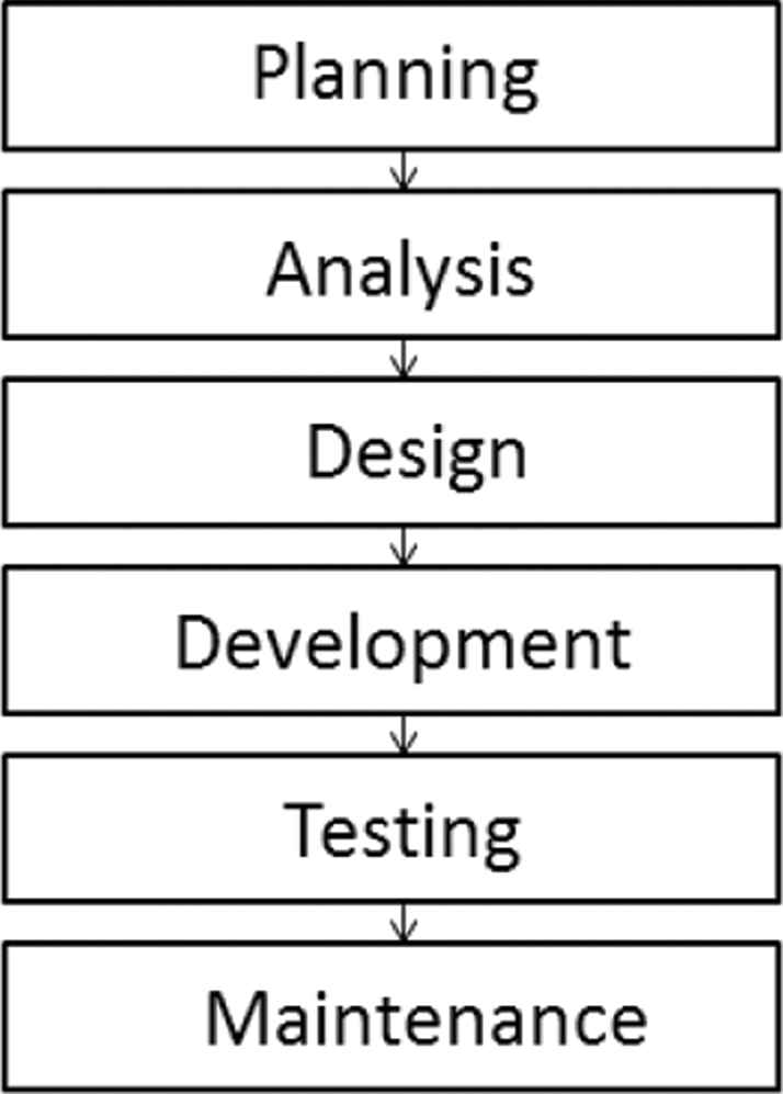
Software engineering sub branches [13].
Enhancing the software testing phase using AI has been an emerging field of research with numerous works done to achieve this target [4,8,14–19]. In these works, researchers reported promising results obtained from applying AI techniques, such as genetic algorithms (GAs) to enhance the software engineering process.
In the next section, a background on program transformation, GAs and particle swarm optimization (PSO) algorithms is reviewed in order to lay a basic foundation to what comes next in this paper. The rest of the paper is organized as follows, Section 3 specifies the problem description, Section 4 will review and highlight the challenges facing program transformation and GAs, Section 5 illustrates the proposed model architecture in detail, Section 6 discusses the experiment settings, Section 7 reviews and discusses the results of this research and finally conclusions are presented in Section 8.
2. BACKGROUND
2.1. Program Transformation
The concept of program transformation can be defined as changing an input program into another program in which the original program's syntax is changed while the original program's semantics is maintained [19–24]. A variety of software engineering areas have been affected by the concept of program transformation including refactoring, reverse engineering [25], software maintenance [26], program comprehension [26], as well as program synthesis. It has been also proved to be a beneficial supporting technology for search-oriented software testing using evolutionary searching algorithms [23,27]. Program transformation applies several small undividable transformation rules to a part or all of the program's source code. Such transformation rules must be semantic equivalence preserving, otherwise the transformation process of the original source code will output a source code that is semantically different from the original program's source code, hence destroy the semantic integrity of both input and output programs. Accordingly, when a researcher attempts to design a program transformation system, they must make sure that the system produces an output program that is semantically equivalent to the input program. To ensure the semantic equivalence of both input and output programs the researcher must make sure that each transformation rule is independently semantic preserving. As a result, if each transformation rule is independently semantic preserving then a whole sequence of these transformation rules will also be semantic equivalence preserving. The efficiency of a transformation system depends on the sequence in which the transformation rules are applied (transformations sequence). For example, two transformation sequences TS1 and TS2 with identical transformation rules (Tr1, Tr2, Tr3) but differ in execution order as follows:
TS1: [Tr1, Tr2, Tr3] and TS2: [Tr2, Tr3, Tr1] may produce different results for the same input program. Cooper et al. [20] referred to this phenomenon as interplay, where a transformation rule may produce opportunities for successive transformation rules and may also eliminate them depending on the order of execution. Most of the transformation systems used today have a fixed sequence of transformation rules to be applied on the input program to serve a specific goal and to target a specific type of programs, which makes it program specific [8]. Such prefixing of the order of transformation rules is not generic and is highly dependent on the input program, which assumes prior knowledge of the target input program.
2.2. Genetic Algorithms
A GA is a Meta heuristic search that imitates the process of natural evolution using evolutionary operators like crossover and mutation to edit a population across several generations toward a stopping criterion, which is usually a maximum number of generations or a specific fitness value. Figure 2 describes the flow of a basic GA.
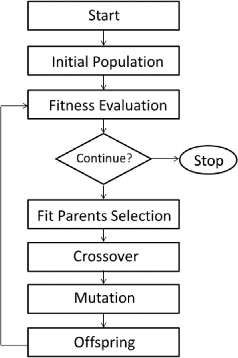
Basic genetic algorithm flow.
First, the problem to be solved must be encoded to be suitable for the GA to work on; more specifically, the target optimization problem's possible solution has to be in the form of a chromosome. A chromosome refers to a possible solution to the optimization problem. A chromosome consists of genes that refer to features of a possible solution. A gene consists of a value picked from a permissible domain of values, such as a chromosome X that contains n genes (G1, G2, …, Gn) implies that a possible solution of the given optimization problem is to execute the contents of the chromosome serially. Once a problem is successfully encoded, a randomly generated initial chromosomes (individuals) are created and referred to as the initial population. Then each member of the initial population passes through a fitness function to evaluate the solution quality or in other words, how good this individual is as a solution to the optimization problem in hand. Once all chromosomes are evaluated, a fitness value for each individual in the initial population will be obtained. According to these fitness values, a collection of individuals will be selected to survive to the next generation. Then the population goes through the process of crossover, where a pair of chromosomes shares their genes according to the probability of crossover Pc so that good genes do not get trapped in a specific chromosome.
Then according to the probability of mutation Pm the population goes through the process of mutation where for each individual, a randomly selected gene is changed within a permissible domain of values hoping to break any possibility of a local optimum solution. Finally, a newly created generation (offspring) is created. This offspring is evaluated by the fitness function. The algorithm then loops until a stopping criterion is reached. Stopping criteria are usually a maximum number of generations or a targeted fitness function value.
2.3. Particle Swarm Optimization
The instinctual behavior performed by members of bird flocks and fish schools allow them to perform precise synchronized movements without colliding, such behavior has been studied in several researches [15,16]. The main idea behind the development of the PSO is the general belief that information sharing among members of a population may result in evolutionary advantages. PSO is a member of the wide category of swarm intelligence methods [17], it was introduced as an optimization method in 1995 [18] to simulate social behavior. One great advantage of PSO is the fact that it is computationally inexpensive since its system requirements are low [17]. Furthermore, it was efficiently applied in a variety of general optimization problems [18] including training of neural networks as well as function optimization. The PSO technique attempts to optimize a given objective function through a population based search. A population in PSO consists of particles, each particle represents a possible solution to the optimization problem, and these particles are a metaphor of fish in fish pools. Particles in a PSO are randomly initialized and allowed to fly freely across a multidimensional search space. During their journey, each particle is allowed to update its own velocity and position according to its best experience reached so far as well as the best experience reached by the entire population. Such updating policy will eventually drive the particle swarm to move toward the area in the search space with the highest objective function value where all particles will gather around the particle (point) with the highest objective function value. First, the initialization step in PSO results in a randomly generated population that is initialized in terms of velocity and position that are set to within a permissible domain of values. Second step is velocity updating where the velocities of all particles are updated according to Equation (1):
Where
Once updated,
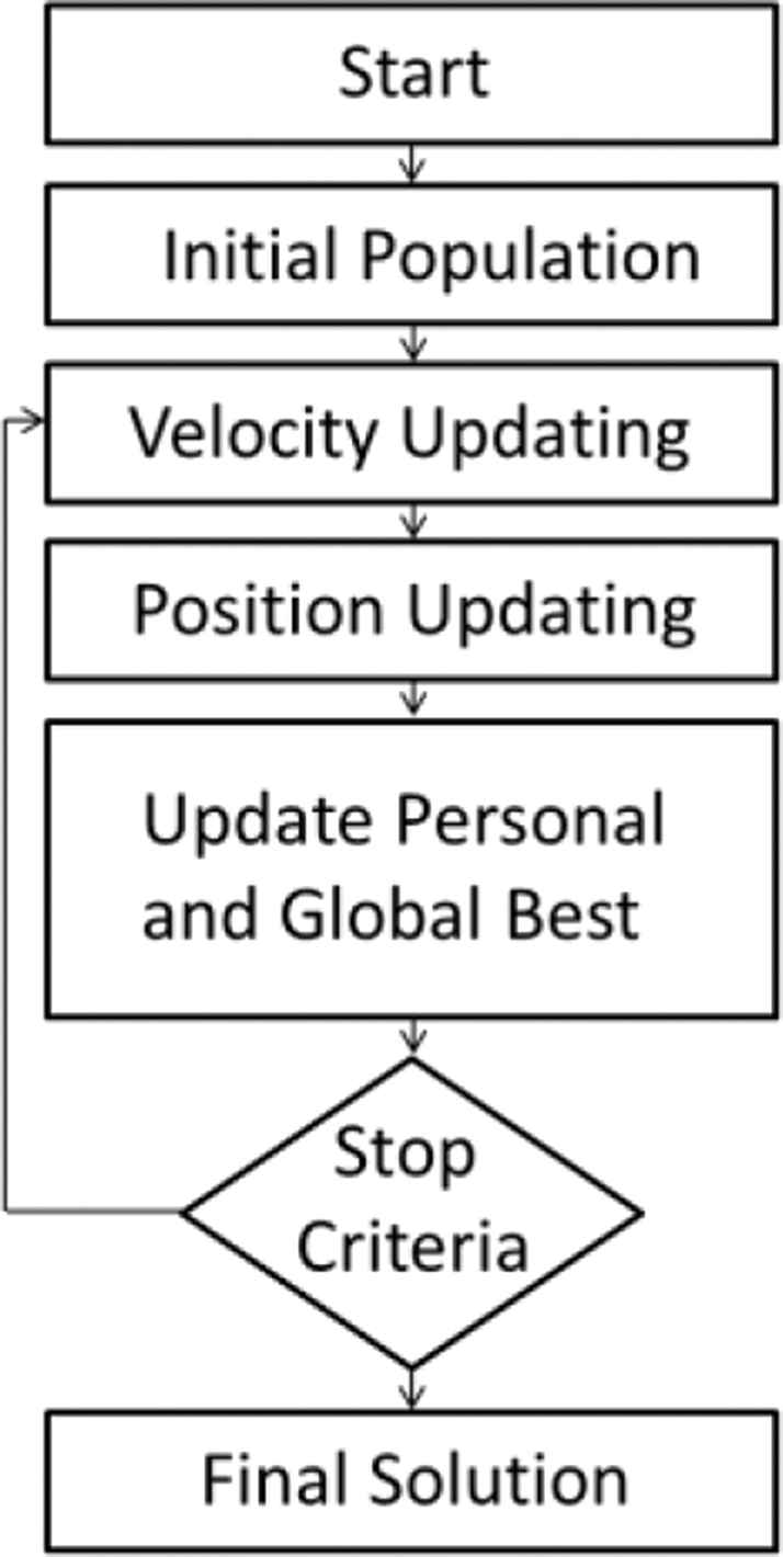
Particle swarm optimization flow.
3. PROBLEM DESCRIPTION
The software development process of applications that run on top of mobile devices is restricted by the limited resources nature of such devices. If a mobile application is developed without taking this point into consideration, the mobile application will not work properly and in extreme cases may not even allow the device to run smoothly. The concept of program transformation has been used to support the process of software engineering [8]; furthermore, AI has been used to automate such a process. Both support and automation processes have suffered from several drawbacks and difficulties [8,9,21,23,24]. Such drawbacks and difficulties are discussed in details in the challenges section.
4. CHALLENGES
4.1. Program Transformation Challenges
The concept of program transformation can be used for various purposes including program environment migration and program optimization. Program environment migration can be referred to as the attempt by a software development team to transfer a program developed specifically for a certain environment to another environment. For example, converting a mobile application that was originally developed for android mobile devices to work on the iOS operated mobile devices. Program optimization targets optimizing a program in terms of various metrics including execution time and program size (number of LoC). In this research, we focus on the use of program transformation to optimize a target program in terms of the number of program's lines of code LoC. To do so, transformation rules are defined and guaranteed to be semantic preserving and are combined together in an order sensitive transformation sequence. Then the transformation sequence would be applied on the program's source code to output a transformed version of the original program. Then the output program is compared with the input program to measure the LoC decline rate to decide how efficient the transformation sequence is to achieve the optimization goal so that it would consume less space on a mobile device's limited storage. After then, the problem is treated as a search problem, such that if there is a transformation rules pool of 30 transformation rules and the length of the transformation sequence is 30 then the possible solution of finding the optimal transformation sequence will exist in a
4.2. GA Challenges
Theoretically, a GA, is supposed to achieve a perfect utilization between each search space exploration and search space exploitation. It was assumed that the population size is infinite, and the fitness function reflects the suitability of a solution accurately and that the genes interactions are minimum [28]. However, although this perfect utilization may be theoretically true for a GA, many problems might exist in practice that raises a number of challenges. For example, the sampling ability of the GA and its performance are affected in practice because the population size is finite. Moreover, a GA may also punish individuals that do not pass the fitness function evaluation by not considering them in the next population. Although these individuals might hold good genes they may still be dropped because a GA fundamentally searches for good chromosomes not good genes. In this case, good genes might be lost in the evolutionary process only because they existed in the wrong chromosome.
5. PROPOSED MODEL ARCHITECTURE
In this section we present a hybrid algorithm that aimed to achieve a global search using GA supported by a fine-grained local search using the PSO algorithm. The idea of this algorithm is to allow GAm to perform global search to generate the initial population, evaluate it and apply genetic operators to generate offspring hoping for a better solution. In the same time, individuals that are rejected by the GA are transferred for rehabilitation to the PSO algorithm where the rejected individuals will communicate as a swarm, share knowledge and update their velocity and position toward a solution that they all, as a swarm agree that it is the best one. Finally, the algorithm would force the rehabilitated individuals back into the GA population to achieve search space exploration as well as search space exploitation.
5.1. Proposed GA
In this subsection we will review the proposed algorithm in details.
5.1.1. Problem encoding
A target input program will be segmented such that each function/subroutine will have a corresponding segment in the chromosome. The following example represents a simple Java code that will be encoded into a chromosome structure so that the GA can operate on it:
public class HelloWorld {
public static void main(String[] args){
subroutine1 ();
subroutine2 ();
}
public static void subroutine1 (){
System.out.println(“Hello, World 1”);
}
public static void subroutine2 (){
System.out.println(“Hello, World 2”);
}
}
Each segment in the above code will be referred to by a unique identifier that's composed by combining a Segment ID and the function's signature (SID + function signature) where SID is an identifier number that will be assigned to each segment and it will be unique, in addition to the function's signature. The previous sample code will be converted into 3 segments:
-Segment #0 main(String[] args)
-Segment #1 subroutine1()
-Segment #2 subroutine2()
Each segment will be led by its ID followed by the sequence of transformation rules to be applied to that segment as shown in Figure 4.
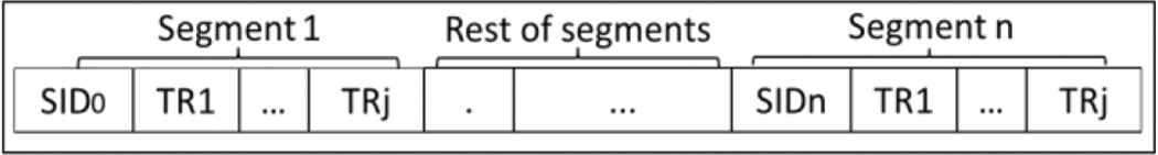
General chromosome structure with segment length j.
5.1.2. Modes of operation
To enable the GA to generate more dynamic solutions, the proposed algorithm will support two modes of operations: Fixed Segment Length (FSL) and Variable Segment Length (VSL). The algorithm can toggle these modes of operation by manipulating the algorithm's parameter VariableSegmentLength that accepts a Boolean value. If false, then the GA will force all segments to be of the same length as shown in Figure 4. If true, then the GA will assign different lengths to each segment derived from the algorithm's learning process as shown in Figure 5.
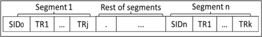
Chromosome with different segment lengths j, k.
To illustrate, the algorithm will start with segment length = 2. Once the optimization result for a specific segment is the same for x generations, the algorithm will attempt to increase the segment length to allow more transformations to take place for that segment otherwise the previous segment length will be mantained.
5.1.3. Population specifications
The initial individuals are generated in families; each family represents a specific segment transformation execution order where each possible segment transformation execution order is represented by a family. For example, family 1 applies transformation for segment 1 then 0 then 2, and family 2 applies transformations for segment 0 then 1 then 2. The segments order is fixed within each family while each segment gets randomly selected transformation rules from the transformation rules pool. The number of transformation rules for each segment will be either fixed or variable depending on the algorithm's mode of operation. Number of families for a given case can be obtained from Equation (5):
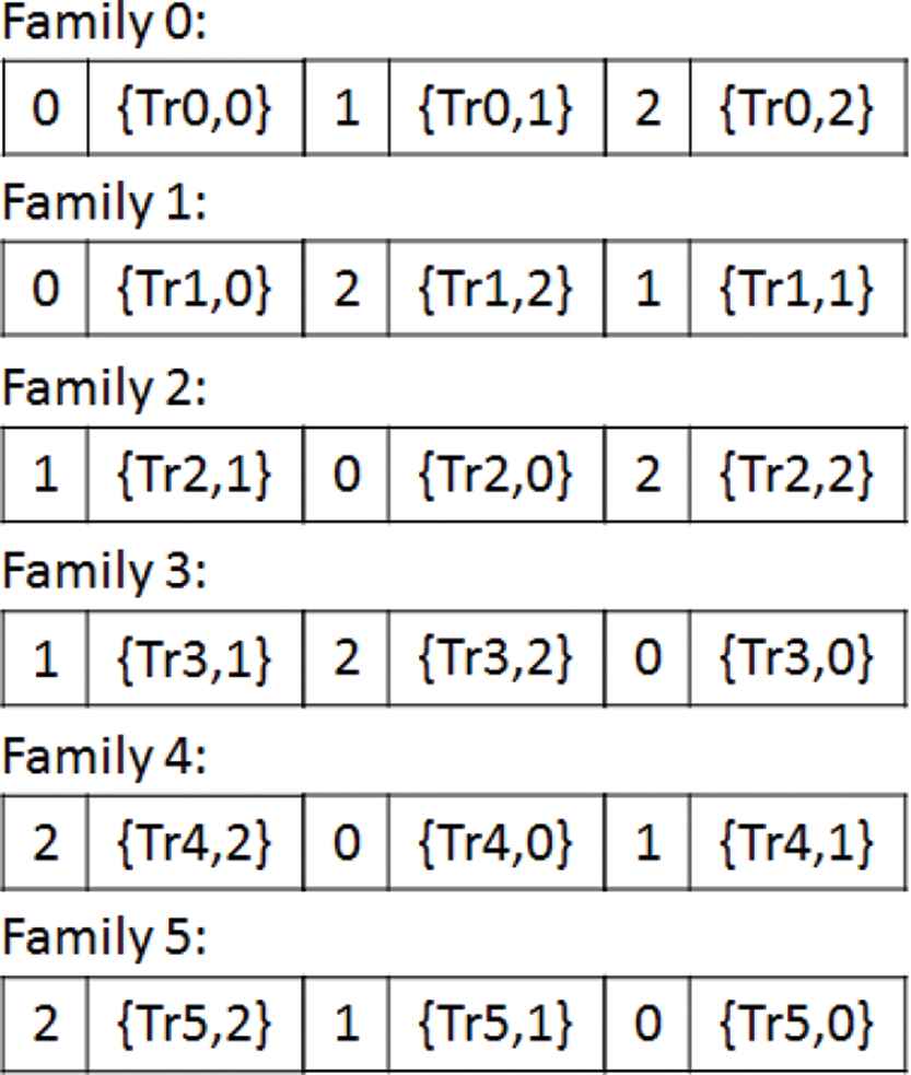
Chromosome families.
5.1.4. Genetic operators
Crossover
Fixed point crossover will be applied such that according to the probability of crossover Pc = 0.7, a random point will be set within each segment so that each segment in parent P1 will be able to share transformation rules with the corresponding segments in parent P2 in both variable and FSL modes of operation as shown in Figures 7 and 8.

FSL crossover example.
VSL crossover example.
Figure 7 shows 2 hypothetical parents in an FSL mode performing a cross over operation where for each segment in the parents a point in the middle of the segment is established and the crossover is performed between each corresponding segments.
Figure 8 shows other hypothetical parents in a VSL mode performing a crossover operation. For each segment in the parents, a random point is set as close as to the idle of each segment and the crossover is performed between each corresponding segments.
Mutation
A combination of random resetting and swap mutation is used in the proposed hybrid algorithm. Random resetting will target the genes within each segment that are holding transformation rules IDs, where such genes will get their values changed from a permissible pool of values according to the probability of transformation rule mutation Pm(Tr) = 0.1 from the pool of predefined transformation rules as shown in Figure 9.
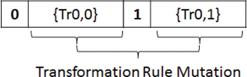
Transformation rules genes mutation.
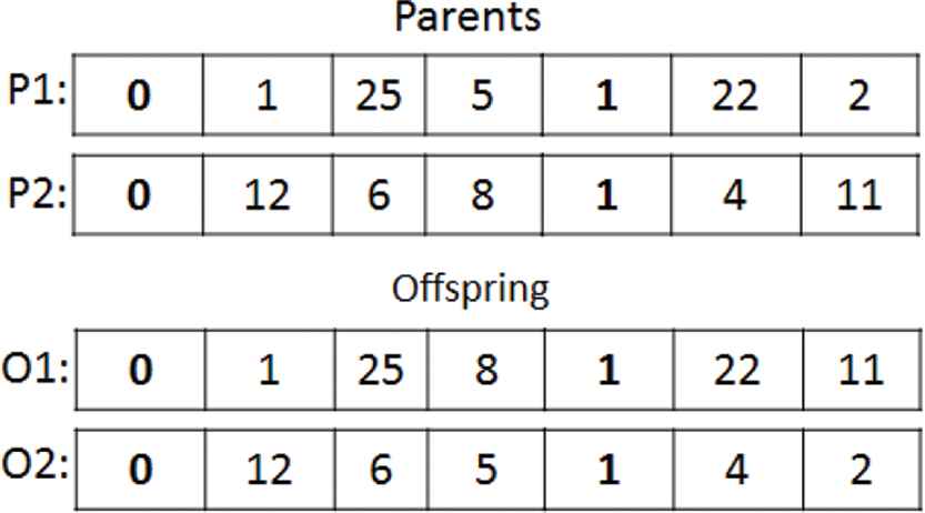
On the other hand, swap mutation will be used to swap segments as a whole according to the probability of segment sequence mutation Pm(Ss) = 0.1 to change the execution order of segments as shown in Figure 10.
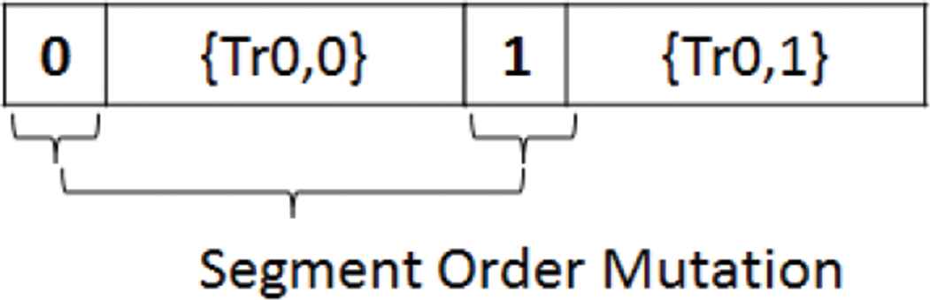
Segment sequence mutation.
Evaluation and selection
The fitness of an individual is measured as the decline rate reached in terms of LoC. An individual will have 2 types on fitness values: one type is for the whole chromosome (Overall fitness of the chromosome) and the other type is a set of fitness values of each segment within the chromosome. This would allow measuring the decline rate when applying the transformation rules of a segment on the source code of that segment and measuring the LoC decline rate between that segment's LoC and the output segment's LoC. According to the chromosome fitness, an individual that achieves a higher LoC decline rate will be selected to survive to the next generation. On the other hand, according to the segment fitness, a chromosome that have high fitness for a specific segment but weak overall fitness as a chromosome, will be transferred to the PSO for rehabilitation. The fitness of a segment in the chromosome can be obtained from Equation (6):
Where SID is the ID of the segment, ILoC is the number of LoC of the input segment and OLoC is the number of lines of code of the output segment, hence, the fitness
Were n is the number of segments in a chromosome.
5.1.5. Segment length increment
As the algorithm runs, if a predetermined number of generations is reached while a segment's fitness value is still the same, the algorithm attempts to increase that segment's length by 1. If no more improvement is reached after this increment, the algorithm maintains the segment's previous length.
5.1.6. Stopping criterion
The proposed algorithm iterates until no improvement in the decline rate of the output program's line of code is reached for a predetermined number of generations:
5.2. PSO Integration
For each generation, the GA's fitness function evaluates all individuals to determine each individual's fitness which is the summation of the fitness of all segments within a chromosome. Think of it as a chromosome that contains a collection of chromosomes (segments) where the fitness of the containing chromosome is the summation of the fitness values of each member chromosome.
Depending on the individual's fitness value, the chromosome will either survive to the next generation or get dismissed. Individuals that will not survive to the next generation will be filtered in such a way that every segment within the individuals will be evaluated independently. Individuals will be classified in n classes where n is the number of segments in the original program and will be transferred to the PSO for rehabilitation. The classifier will assure a fair distribution for individuals transferred to the PSO such that the rejected individuals will be classified into a number of classes, the classifier will make sure that at least one individual from each class is selected to be transferred to the PSO and will limit the number of individuals transferred for rehabilitation to 50% of the rejected individuals.
The classifier used in this research is a linear classifier (Naive Bayes) as it's simple and easy to build. PSO will work in two modes: the first one is an online mode in which the PSO works side by side with the genetic algorithm such that when the PSO acquires the final rehabilitation result it will return back to the GA. If the GA has terminated, the PSO will force it to start back while pushing the rehabilitated individual to replace the weakest individual in the last generation reached by the GA. If the GA has not terminated yet, the PSO will push the rehabilitated individual to replace the weakest individual in the current offspring.
As for the offline mode, the PSO rehabilitation process will start only when the GA terminates. The PSO search space will consist of n partitions, where n is the number of segments in the targeted program. Each partition will contain members that share the same segment with high LoC decline rate. Finally, the PSO members will communicate to update their velocity and position to achieve the best possible result.
The velocity of a particle reflects the distance traveled by this particle at a given iteration; it depends on the previous position found by the particle itself and the best solution found by the whole swarm. The position of a particle represents the currently targeted point in the search space that it traverses, the change of a particle's velocity reflects in a change of its position to attempt to reach a better solution. Below is the algorithm that describes the PSO integration:
Input: List <Individual>: rejected individuals from GA.
Output: Rehabilitated Individual.
Variables: V: Velocity, P: Position, i: individual#, j: iteration#. GB: global best, PB: personal best.
Process:
Begin
Initialize PSO.Population = Input
Foreach (Individual INDi in Input)
Calculate: V(INDij) & PB(INDij)
If(PB(INDij) < GB)
GB = INDij
Else
If(j =Iteration Limit)
Output = GB & break
Else
Calculate: P(INDij) & V(INDij)
i++ & j++
Continue
End Foreach
Return Output
END
In the algorithm above, V, P, PB and GB are calculated according to Equations in (1) to (4). First the algorithm is initialized with the rejected individuals from the GA, then the algorithm iterates through each individuals and calculates the velocity and personal best then the personal best is compared against the global best such that the global best will be overwritten with the personal best if the personal best achieves better result than the global best, otherwise the algorithm's iterations limit is checked such that the algorithm will output the global best and breaks if the iterations limit is reached, otherwise the algorithm will calculate the new position and velocity, increment i and j and continue. In the end, the algorithm returns the individual that all swarm members agree that it's the best solution. The rehabilitation process ends when the PSO members agree that the best possible result is reached. The optimal individual will be transferred back to the GA and either resume the algorithm or replace the weakest individual in the current offspring as explained earlier, Figure 11 shows the integration of GA and PSO in the proposed hybrid algorithm.
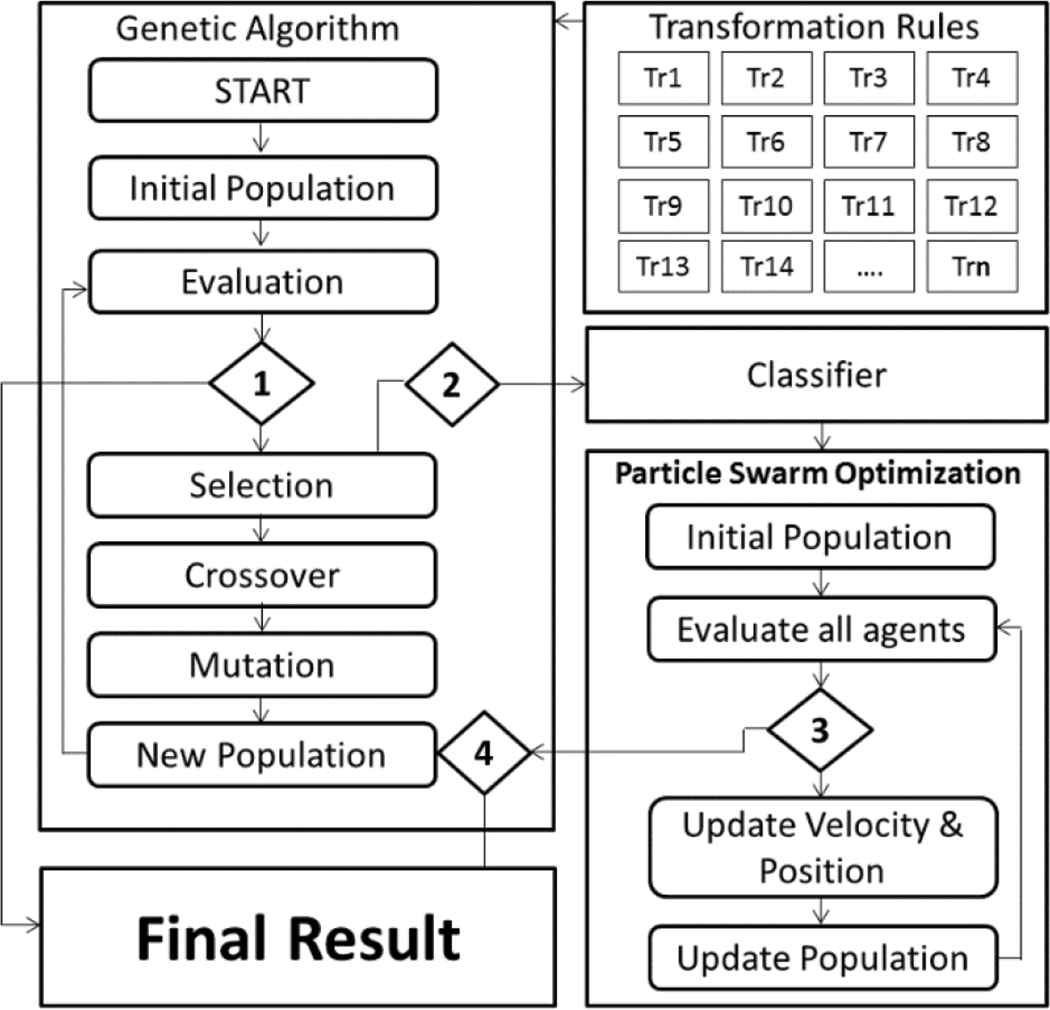
Proposed hybrid genetic algorithm flow.
6. EXPERIMENT SETTINGS
Six experiments were conducted on different cases while varying the following: 1. algorithm type (either a GA or a hybrid GA); 2. GA's mode (either FSL or VSL); 3. PSO algorithm's mode (either online (ON) or offline (OFF) or not available (NA) in the cases of using nonhybrid GA). Table 1 explains the six different experiments used in this research.
| Experiment# | Algorithm | GA Mode | PSO Mode |
|---|---|---|---|
| 1 | GA | FSL | NA |
| 2 | GA | VSL | NA |
| 3 | HGA | FSL | OFF |
| 4 | HGA | FSL | ON |
| 5 | HGA | VSL | OFF |
| 6 | HGA | VSL | ON |
FSL, Fixed Segment Length; GA, genetic algorithm; HGA, hybrid genetic algorithm; NA, not available; OFF, offline; ON, online; VSL, Variable Segment Length
Experimental cases.
The original program's source code contains a total of 147 LoC; the six experiments mentioned in Table 1 were conducted to reach the least possible LoC in the transformed program. Results from conducting Experiments 1 and 2 are displayed in Tables 2 and 3, respectively. In Experiments 3–6, the proposed hybrid GA was used with different types of segment length and PSO modes of operation.
| Modes |
LoC |
|||||||
|---|---|---|---|---|---|---|---|---|
| # | A | SL | PSO | In | Out | Out to In (%) | Decline (%) | ITR |
| 1 | GA | F | NA | 147 | 122 | 82.99 | 17.01 | 56 |
| 2 | GA | F | NA | 147 | 124 | 84.35 | 15.65 | 59 |
| 3 | GA | F | NA | 147 | 126 | 85.71 | 14.29 | 45 |
| 4 | GA | F | NA | 147 | 130 | 88.44 | 11.56 | 64 |
| AVG | 125.5 | 85.37 | 14.63 | 56 | ||||
GA, genetic algorithm; ITR, number of iterations; LoC, Lines of Code; NA, not available; PSO, Particle Swarm Optimization
Results for Experiment 1.
| Modes |
LoC |
|||||||
|---|---|---|---|---|---|---|---|---|
| # | A | SL | PSO | In | Out | Out to In (%) | Decline (%) | ITR |
| 1 | GA | V | NA | 147 | 116 | 78.91 | 21.09 | 67 |
| 2 | GA | V | NA | 147 | 120 | 81.63 | 18.37 | 65 |
| 3 | GA | V | NA | 147 | 124 | 84.35 | 15.65 | 62 |
| 4 | GA | V | NA | 147 | 126 | 85.71 | 14.29 | 61 |
| AVG | 121.5 | 82.65 | 17.35 | 64 | ||||
GA, genetic algorithm; ITR, number of iterations; LoC, Lines of Code; NA, not available; PSO, Particle Swarm Optimization
Results for Experiment 2.
The results are displayed in Tables 4–7. “Modes A” refers to the used algorithm either a normal GA or a hybrid genetic algorithm (HGA). “Modes SL” refers to the segment length mode either VSL (V) or FSL (F). “Modes PSO” refers to the PSO algorithm's mode either online (ON) or offline (OFF). “LoC In” refers to the Lines of Code of the input program while “LoC Out” refers to the Lines of Code of the output program.
| Modes |
LoC |
|||||||
|---|---|---|---|---|---|---|---|---|
| # | A | SL | PSO | In | Out | Out to In (%) | Decline (%) | ITR |
| 1 | HGA | F | OFF | 147 | 98 | 66.67 | 33.33 | 39 |
| 2 | HGA | F | OFF | 147 | 102 | 69.39 | 30.61 | 35 |
| 3 | HGA | F | OFF | 147 | 106 | 72.11 | 27.89 | 36 |
| 4 | HGA | F | OFF | 147 | 109 | 74.15 | 25.85 | 38 |
| AVG | 103.75 | 70.58 | 29.42 | 37 | ||||
HGA, hybrid genetic algorithm; ITR, number of iterations; LoC, Lines of Code; PSO, Particle Swarm Optimization
Results for Experiment 3.
| Modes |
LoC |
|||||||
|---|---|---|---|---|---|---|---|---|
| # | A | SL | PSO | In | Out | Out to In (%) | Decline (%) | ITR |
| 1 | HGA | F | ON | 147 | 96 | 65.31 | 34.69 | 27 |
| 2 | HGA | F | ON | 147 | 101 | 68.71 | 31.29 | 23 |
| 3 | HGA | F | ON | 147 | 102 | 69.39 | 30.61 | 24 |
| 4 | HGA | F | ON | 147 | 106 | 72.11 | 27.89 | 26 |
| AVG | 101.25 | 68.88 | 31.12 | 25 | ||||
HGA, hybrid genetic algorithm; ITR, number of iterations; LoC, Lines of Code; ON, online; PSO, Particle Swarm Optimization
Results for Experiment 4.
| Modes |
LoC |
|||||||
|---|---|---|---|---|---|---|---|---|
| # | A | SL | PSO | In | Out | Out to In (%) | Decline (%) | ITR |
| 1 | HGA | V | OFF | 147 | 76 | 51.70 | 48.30 | 43 |
| 2 | HGA | V | OFF | 147 | 78 | 53.06 | 46.94 | 39 |
| 3 | HGA | V | OFF | 147 | 79 | 53.74 | 46.26 | 41 |
| 4 | HGA | V | OFF | 147 | 83 | 56.46 | 43.54 | 42 |
| AVG | 79 | 53.74 | 46.26 | 42 | ||||
HGA, hybrid genetic algorithm; ITR, number of iterations; LoC, Lines of Code; OFF, offline; PSO, Particle Swarm Optimization
Results for experiment 5.
| Modes |
LoC |
|||||||
|---|---|---|---|---|---|---|---|---|
| # | A | SL | PSO | In | Out | Out to In (%) | Decline (%) | ITR |
| 1 | HGA | V | ON | 147 | 62 | 42.18 | 57.82 | 27 |
| 2 | HGA | V | ON | 147 | 67 | 45.58 | 54.42 | 31 |
| 3 | HGA | V | ON | 147 | 75 | 51.02 | 48.98 | 28 |
| 4 | HGA | V | ON | 147 | 87 | 59.18 | 40.82 | 30 |
| AVG | 72.75 | 49.49 | 50.51 | 29 | ||||
HGA, hybrid genetic algorithm; ITR, number of iterations; LoC, Lines of Code; ON, online; PSO, Particle Swarm Optimization
Results for Experiment 6.
“Out to In” refers to the percentage of the output program compared to the input program. “Decline” refers to the decline rate achieved by the test case that's measured as the ratio of the number of deleted LoC to the “LoC In.” “ITR” refers to the number of iterations consumed by the GA until convergence. The proposed algorithm was executed on a 2.6 GHz Intel Core i7 vPro machine with 16 GB of RAM and a magnetic HDD on a 64 bit OS.
7. RESULTS
The above results show that the proposed hybrid algorithm was able to overcome the basic GA in terms of the transformed program LoC. The significant changes appeared when switching from a normal GA to the hybrid GA. There was also a significant change with the hybrid GA when switched from FSL to VSL, and so affected the decline rate. On the other hand, the GA iterations increased for the normal GA when switched from FSL to VSL due to the increase in the chromosome length that expanded the search space. The average number of iterations decreased significantly when the GA was combined with the PSO as it made the search more efficient, hence led to less iteration of GA. However, the same phenomenon of the increase of number of iterations when switching from FSL to VSL is witnessed in the hybrid GA, this can be described as the trade-off between achieving the lowest possible LoC decline rate and the GA performance. The best result acquired when trying to reach the highest decline rate was achieved in Experiment 6, however, Experiment 4 allowed less iteration in the GA but with lower decline rate. The final results acquired from Table 8 are visualized in Figures 12–15.
| Modes |
LoC |
||||||
|---|---|---|---|---|---|---|---|
| # | A | SL | PSO | Out | Out to In (%) | Decline (%) | ITR |
| 1 | GA | F | NA | 125.5 | 85.37 | 14.63 | 56 |
| 2 | GA | V | NA | 121.5 | 82.65 | 17.35 | 64 |
| 3 | HGA | F | OFF | 103.75 | 70.58 | 29.42 | 37 |
| 4 | HGA | F | ON | 101.25 | 68.88 | 31.12 | 25 |
| 5 | HGA | V | OFF | 79 | 53.74 | 46.26 | 42 |
| 6 | HGA | V | ON | 72.75 | 49.49 | 50.51 | 29 |
GA, genetic algorithm; HGA, hybrid genetic algorithm; ITR, number of iterations; LoC, Lines of Code; NA, not available; OFF, offline; ON, online; PSO, Particle Swarm Optimization
Combined results for Experiments 1–6.
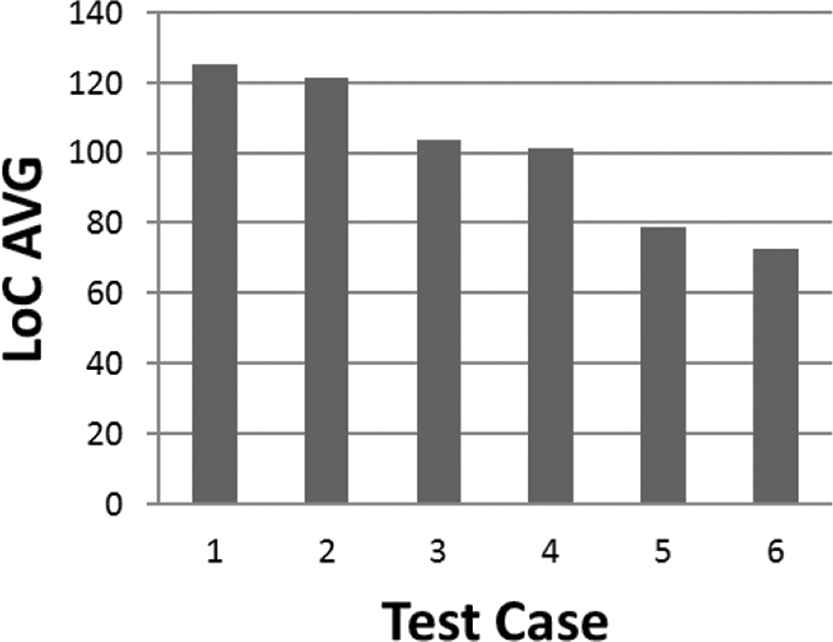
Output lines of code average for all 6 experiments.
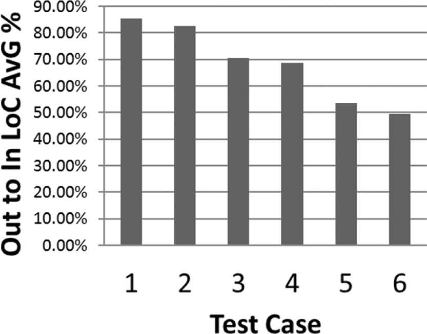
Output to input lines of code average.
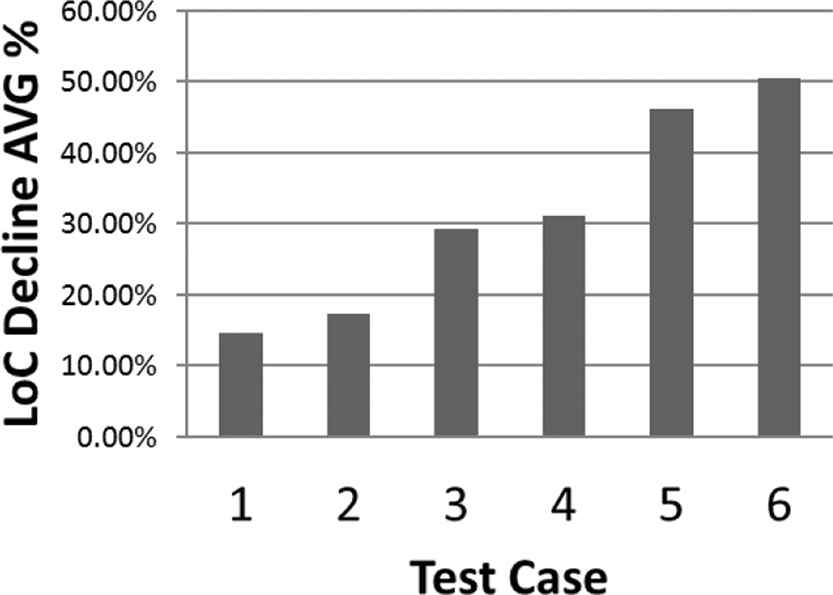
Lines of code decline rate average.

Genetic algorithm average iterations.
8. CONCLUSION
When automating the optimization process of a program in terms of LoC, we should not transform a program that contains multiple sub routines as a whole. As we suppose that a large multi-part program may contain many subroutines where each subroutine needs a specific transformation rules to be applied on it in a specific order. Hence, linear transformation will not be efficient. When combining the transformation sequences to be applied in each segment (sub routine/part of a programs) in a chromosome structure as mentioned in Section 4.1, we will get a transformation sequence that includes n number of segments were each segment includes its own transformation.
A combination of AI techniques has been utilized in this research to evolve program transformation sequences to achieve the highest possible decline rate in terms of the transformed program's LoC. A GA was utilized to perform a global search supported by the PSO algorithm to perform a local search so that a balance between search space exploration and search space exploitation was achieved. The idea of expanding the chromosome segment's length targeted a more flexible and dynamic search space to achieve the highest possible LoC decline rate; however, it may not be suitable for small programs that do not require intense transformations, as the algorithm may end up with useless extra genes in each segment in the chromosome. In VSL mode, as the chromosome's length expands, new genes enter the chromosome structure that allows the possibility to achieve a better result in terms of LoC decline rate; however, the GA may consume more iteration to converge as the chromosome gets larger.
Currently, the algorithm only expands the segment length when no better result is reached for a predetermined number of generations. More research is needed to optimize the criteria upon which the algorithm decides to expand the segment length in order to make more balance between the increase of the segment length and the increase of the number of iterations in the GA. More research is needed to decide the relation between the size of the transferred rejected individuals for rehabilitation and the algorithm's solution's LoC decline rate and iterations consumed.
CONFLICT OF INTEREST
Authors have no conflict of interest to declare.
REFERENCES
Cite this article
TY  - JOUR
AU  - Ahmed Maghawry
AU  - Mohamed Kholief
AU  - Yasser Omar
AU  - Rania Hodhod
PY  - 2020
DA  - 2020/02/20
TI  - An Approach for Evolving Transformation Sequences Using Hybrid Genetic Algorithms
JO  - International Journal of Computational Intelligence Systems
SP  - 223
EP  - 233
VL  - 13
IS  - 1
SN  - 1875-6883
UR  - https://doi.org/10.2991/ijcis.d.200214.001
DO  - 10.2991/ijcis.d.200214.001
ID  - Maghawry2020
ER  -