International Journal of Computational Intelligence Systems

Volume 13, Issue 1, 2020, Pages 310 - 317

Hierarchical Bayesian Choice of Laplacian ARMA Models Based on Reversible Jump MCMC Computation

Authors
Suparman*
Department of Mathematics Education, Universitas Ahmad Dahlan, Yogyakarta, Indonesia
Corresponding Author
Suparman
Received 19 December 2019, Accepted 20 February 2020, Available Online 18 March 2020.
DOI
10.2991/ijcis.d.200310.006How to use a DOI?
Keywords
ARMA time series; Hierarchical Bayesian; Laplacian noise; Reversible jump MCMC
Abstract

An autoregressive moving average (ARMA) is a time series model that is applied in everyday life for pattern recognition and forecasting. The ARMA model contains a noise which is assumed to have a specific distribution. The noise is often considered to have a Gaussian distribution. However in applications, the noise is sometimes found that does not have a Gaussian distribution. The first objective is to develop the ARMA model in which noise has a Laplacian distribution. The second objective is to estimate the parameters of the ARMA model. The ARMA model parameters include ARMA model orders, ARMA model coefficients, and noise variance. The parameter estimation of the ARMA model is carried out in the Bayesian framework. In the Bayesian framework, the ARMA model parameters are treated as a variable that has a prior distribution. The prior distribution for the ARMA model parameters is combined with the likelihood function for the data to get the posterior distribution for the parameter. The posterior distribution for parameters has a complex form so that the Bayes estimator cannot be determined analytically. The reversible jump Markov chain Monte Carlo (MCMC) algorithm was adopted to determine the Bayes estimator. The first result, the ARMA model can be developed by assuming Laplacian distribution noise. The second result, the performance of the algorithm was tested using simulation studies. The simulation shows that the reversible jump MCMC algorithm can estimate the parameters of the ARMA model correctly.

Copyright
© 2020 The Authors. Published by Atlantis Press SARL.
Open Access
This is an open access article distributed under the CC BY-NC 4.0 license (http://creativecommons.org/licenses/by-nc/4.0/).

1. INTRODUCTION

An autoregressive moving average (ARMA) is a time series model that is applied to modeling and forecasting in various fields, for example, [13]. The ARMA model is used in the field of short-term load system for forecasting [1]. The ARMA model is used in the field of science for forecasting wind speed [2]. The ARMA model is used in the business field for modeling volatility and risk of shares financial markets [3].

This ARMA model contains a noise. This noise is assumed to have a specific distribution. Noise for ARMA models is often considered to have a Gaussian distribution, for example, [47]. The ARMA model is used for sequential and non-sequential acceptance sampling [4]. The ARMA model is used to investigate the non-residual residual surges [5]. The ARMA model is used to predict small-scale solar radiation [6]. The ARMA model is used to forecast passenger service charge [7]. In an ARMA model application, the noise sometimes shows that it does not have a Gaussian distribution. Several studies related to ARMA models with non-Gaussian noise can be found in [13,8,9]. Estimating ARMA parameters with non-Gaussian noise is investigated using high-order moments [8]. A cumulant-based order determination of ARMA models with Gaussian noise is studied in [9].

A Laplacian is a noise investigated by several authors, for example, [1012]. If x is a random variable with a Laplace distribution then x has a probability function:

f(x|δ,β)=12βexp|xδ|β.(1)

Here, δ is a location parameter and β>0 is a scale parameter. The Laplacian noise is used to detect body position changes [10]. The feasibility pump algorithm is used to find the sparse representation under Laplacian noise [11]. Laplacian noise is used in human sensory processing [12]. However, the ARMA model that contains Laplacian noise has not been studied. The significant novelty of the proposed study is the use of a Laplacian noise in the ARMA model. The Laplacian noise provides a smaller error variance compared to Gaussian noise. This study has several objectives. The first objective is to develop the new ARMA model by assuming that noise has a Laplacian distribution. The second objective is to estimate the order of the ARMA model. The third objective is to estimate the ARMA model coefficients.

If the ARMA model is compared to the AR model and the MA model, the ARMA model is a more general model than the AR model and the MA model. If the ARMA model is compared to the ARIMA model, the only difference is the integrated part. Integrated refers to how many times it takes to differentiate a series to achieve stationary condition. The ARMA model is equivalent to the ARIMA model of the same MA and AR orders with no differencing. An ARMA model was chosen instead of the other models such as AR model, MA model, or ARIMA model because the ARMA model can describe a more general class of processes than AR model and MA model. The ARMA model in this study has stationary and invertible properties that are not possessed by the ARIMA model.

This paper consists of several parts. The first part gives an introduction regarding the ARMA model and its application. The second part explains the method used to estimate the ARMA model. The third part presents the results of the research and discussion. The fourth section gives some conclusions and implications.

2. MATERIALS AND METHODS

This paper uses an ARMA model that has Laplacian noise. The parameters used in ARMA model are the order of the ARMA model, the coefficients of the ARMA model, and the variance of the noise. The parameter estimation of the ARMA model is carried out in the Bayesian framework. The first step determines the likelihood function for data. The second step determines the prior distribution for the ARMA model parameters. The reason about the consideration of prior distribution is to improve the quality of parameter estimation. The prior distribution can be determined from previous experiments. The Binomial distribution is chosen as the prior distribution for ARMA orders. The uniform distribution is selected as the prior distribution for the ARMA model coefficient. The inverse Gamma distribution is selected as the prior distribution for the noise parameter. The third step combines the likelihood function for data with the prior distribution to get the posterior distribution. The fourth step determines the Bayes estimator based on the posterior distribution using the reversible jump Markov chain Monte Carlo (MCMC) algorithm [13]. Time series modeling via reversible jump MCMC is a very well studied topic in the literature [14,15]. The power of reversible jump MCMC algorithm is in the fact that it can move between space of varying dimension and not that it is just a simple MCMC method. The fifth step tests the performance of the reversible jump MCMC algorithm by using simulation studies.

3. RESULTS AND DISCUSSION

This section discusses the likelihood function for data, Bayesian approach, reversible jump MCMC algorithm, and simulations.

3.1. Likelihood Function

Suppose that x1,,xn are n data. This data is said to have an autoregressive model if for t=1,,n the data satisfies the following equation:

xt=i=1pϕixti+j=1qθjztj+zt(2)

The values of p and q are orders for the ARMA model. To abbreviate the mention, the ARMA model that has the order p and q will be written by ARMA(p,q). Given the values of orders p and q, the values ϕ1,,ϕp and θ1,,θq express the coefficients of the ARMA(p,q). While the random variables z1,,zn are noise. This noise is assumed to have a Laplace distribution with mean 0 and variance 2β2. The probability function for the variable zt is written by the following equation:

g(zt|β)=12βexp|zt|β.(3)

With a variable transformation between xt and zt, the probability function for the variable xt can be written by

fxt|β=12βexp|i=1pϕixtij=1qθjztj+xt|β.(4)

Suppose that x=x1,,xn, ϕp=ϕ1,,ϕp and θq=ϕ1,,ϕq. The probability function for x is

fx|p,q,ϕ(p),θ(q),β=t=p+1n12βexp|i=1pϕixtij=1qθjztj+xt|β=12βnpexp1βt=p+1n|i=1pϕixtij=1qθjztj+xt|.(5)

The ARMA(p,q) model is called stationary if and only if the root equation is located outside the unit circle. The stationarity of ARMA(p,q) model refers to the mean, variance, and autocorrelation are all constant over time. Suppose that Sp denotes the stationarity region. This stationary condition is difficult to determine if the order value p is high. To overcome this problem, a transformation is made. Let F be a transformation from ϕ(p)Sp to r=r1,,rp1,1p where r1,,rp are functions of partial autocorrelation [16]. With the F transformation, this stationary condition of the ARMA(p,q) model becomes easily determined even though the order value p is high. The ARMA(p,q) model is called stationary if and only if r1,,rp1,1p.

The ARMA(p,q) model is called invertible if and only if the root of equation 01+j=1qθjBj=0 is located outside the unit circle. The invertibility of ARMA(p,q) model refers to the noises can be inverted into a representation of past observations. The limitation of the ARMA(p,q) model is that if the ARMA(p, q) model is not invertible, the ARMA(p, q) model cannot be used to forecast the future values of the dependent. Suppose Iq denotes an invertible region. This invertibility condition is difficult to determine if the order q value is high. To overcome this problem, a transformation is made. Let G be a transformation from θ(q)Iq to ρ=ρ1,,ρq1,1q where ρ1,,ρq are functions of inverse partial autocorrelation [17]. With the G transformation, the invertibility condition of the ARMA(p,q) model is easily determined even though the order q value is high. The ARMA(p,q) model is called invertible if and only if ρ1,,ρq1,1q. If the likelihood function for data is expressed in the transformation of F and G, the likelihood function for data can be written by

f(x|p,q,r(p),ρ(q),β)=t=p+1n12βexp|i=1pF1(ri)xtij=1qG1(ρj)ztj+xt|β=(12β)npexp1βt=p+1n|i=1pF1(ri)xtij=1qG1(ρj)ztj+xt|.(6)

In the probability function for this data, F1 and G1 are inverse transformations for the transformation of F and G.

3.2. Prior and Posterior Distributions

The Binomial distribution with the parameter λ is chosen as the prior distribution for order p. The prior distribution for order p can be written by

πp|λ=Cppmaxλp(1λ)pmaxp(7)
where the pmax value is set. Whereas the Binomial distribution with the parameter μ is chosen as the prior distribution for order q. The distribution of priors for q order can be expressed by
πq|μ=Cqqμq(1μ)qmaxq(8)
where the value qmax is set. For model order p and q, a Binomial distribution is used because it is a conjugate prior.

The prior distribution for r(p) given by the order p is a uniform distribution at (1,1)p. The uniform distribution is chosen because it is a conjugate prior. The prior distribution for r(p) if given an order p can be written by

π(r(p)|p)=12p.(9)

The prior distribution for ρ(q) given by the order q is a uniform distribution at (1,1)q. The prior distribution for ρ(q) if given an order q can be written by

π(ρ(q)|q)=12q.(10)

The inverse Gamma distribution with parameter v is selected as the prior distribution for β. Value u is set, namely: u=1. The distribution of prior for β can be expressed by

π(β|u,ν)=νuΓ(u)β(u+1)expvβ.(11)

For β, an inverse Gamma distribution is used because it is a conjugate prior.

This prior distribution contains a parameter, namely: λ,μ, and ν. Uniform distribution at interval (0,1) is chosen as the prior distribution for λ, namely: π(λ)=1. The uniform distribution at interval (0,1) is chosen as the prior distribution for μ, namely: π(μ)=1. The uniform distribution is proposed in previous work [7].

Finally, the Jeffreys distribution is chosen as the prior distribution for ν. The prior distribution for ν can be written by π(ν)1ν. This is a non-informative prior distribution. Thus, the joint prior distribution for p,q,r(p),ρ(q),λ,μ,β, and ν can be expressed by

π(p,q,r(p),ρ(q),λ,μ,β,v)Cppmaxλp(1λ)pmaxpCqqmaxμq(1μ)qmaxq12(p+q)νuΓ(u)β(u+1)expvβ1β1ν.(12)

By using the Bayes theorem, distribution posterior for p,q,r(p),ρ(q),λ,μ,β, and ν can be expressed by

π(p,q,r(p),ρ(q),λ,μ,β,v|x)  (12β)npexp1βt=p+1n|i=1pF1(ri)xti    j=1qG1(ρj)ztj+xt|    Cppmaxλp(1λ)pmaxpCqqmaxμq(1μ)qmaxq12(p+q)νuΓ(u)β(u+1)    expvβ1β1ν  (12)np(1β)np1exp   1βt=p+1n|i=1pF1(ri)xtij=1qG1(ρj)ztj+xt|    Cppmaxλp(1λ)pmaxpCqqmaxμq(1μ)qmaxq12(p+q)νu1Γ(u)β(u+1)    expvβ.(13)

This posterior distribution has a complex form so that the Bayes estimator cannot be determined explicitly. The reversible jump MCMC algorithm was adopted to determine the Bayes estimator.

3.3. Reversible Jump MCMC

The basic idea of the MCMC algorithm is to treat the parameters p,q,r(p),ρ(q),λ,μ,β, and ν as a Markov chain. To determine the Bayes estimator for parameters, a Markov chain is created by simulation. This Markov chain is designed so that it has a limit distribution that approaches the posterior distribution for parameters p,q,r(p),ρ(q),λ,μ,β, and ν. This Markov chain is used to find the Bayes estimator. The algorithm consists of two stages, namely; the first stage is to create a Markov chain for λ,μ,β,ν|p,q,r(p),ρ(q) by simulation. The second stage makes the Markov chain for p,q,r(p),ρ(q)|λ,μ,β,ν by simulation.

Distribution for λ,μ,β,ν|p,q,r(p),ρ(q) is the product of the distribution for λ|p,q,r(p),ρ(q), the distribution for μ|p,q,r(p),ρ(q), distribution for β|p,q,r(p),ρ(q), and the distribution for ν|p,q,r(p),ρ(q). The distribution for λ|p,q,r(p),ρ(q) is Binomial, the distribution for μ|p,q,r(p),ρ(q) is Binomial, the distribution for β|p,q,rp,ρq is the Gamma inverse distribution, distribution for ν|p,q,rp,ρq is the Gamma distribution. Simulation for the Markov chain λ,μ,β,ν|p,q,r(p),ρ(q) is as follows [18]:

λBp+1,pmaxp+1,
μBq+1,qmaxq+1,
βIG(np,v+t=p+1n|i=1pF1(ri)xtij=1qG1(ρj)ztj+xt|),
υG(u,1β).

The distribution for p,q,r(p),ρ(q)|λ,μ,β,ν has a complex form. Simulation for the Markov chain p,q,r(p),ρ(q)|λ,μ,β,ν is carried out using the reversible jump MCMC algorithm. The reversible jump MCMC algorithm is an extension of the Metropolis–Hastings algorithm [19,20]. This reversible jump MCMC algorithm uses six types of transformation, namely: birth for order p, death for order p, change for coefficient r(p), birth for order q, death for order q, and change for coefficient ρ(q).

3.4. Birth of the Order p

Suppose that w=p,q,r(p),ρ(q) is the old Markov chain and w=p,q,rp,ρ(q) is a new Markov chain. The birth of the order p changes the order p and the coefficient r(p) but does not change the order q and the coefficient ρ(q). The new Markov chain p,q,rp,ρ(q) is defined as follows: (a) first determine the order p=p+1, (b) the second takes randomly a at the interval 1,1 and then determines rp=r(p),a. The old Markov chain will be replaced by a new Markov chain with probability

ηpAR(w,w)=min{1,f(x|w)f(x|w)π(p)π(p)π(r(p)|p)π(r(p)|p)q(w,w)q(w,w)}(14)
where f(x|w)f(x|w) is the ratio of the likelihood function, π(p)π(p) is the ratio between the prior distribution for order p and p, π(r|p)π(r|p) is the ratio between the posterior distribution for rp and r(p), and q(w,w)q(w,w) is the ratio between the distribution of w and w. In contrast, the old Markov chain will remain with the probability 1ηpARw,w. Following is the calculation for the probability function ratio, the ratio between the prior distribution for order p and p, the ratio between the posterior distribution for rp and r(p), and the ratio between the distribution of w and w.

The ratio for likelihood function can be stated by

fx|p,q,rp,ρ(q)fx|p,q,r(p),ρ(q)=exp1βt=p+1n|i=1pF1rixtij=1qG1(ρj)ztj+xt|exp1βt=p+1n|i=1pF1(ri)xtij=1qG1(ρj)ztj+xt|12β.(15)

The ratio between the prior distribution for order p and p can be expressed by

π(p)π(p)=pmaxpp+1λ1λ.(16)

The ratio between posterior distribution for order p and p can be written by

π(r(p)|p)π(r(p)|p)=12.(17)

While the ratio between the distribution of w and w depends on the value of a. If a<0, the ratio between the distribution of w and w can be written by

q(w,w)q(w,w)=1a+1.(18)

If a>0, the ratio between the distribution of w and w can be written by

q(w,w)q(w,w)=11a.(19)

3.5. Death of the Order p + 1

Death of the order p+1 is the opposite of the birth of order p. Let w=p,q,r(p+1),ρ(q) be the old Markov chain and w=p,q,rp,ρ(q) is a new Markov chain. The death of the order p+1 changes the order p+1 and the coefficient r(p+1) but does not change the order and the coefficient ρ(q). The new Markov chain p,q,rp,ρ(q) is defined as follows: (a) first determine the order p=p, (b) the second determines rp=r(p). The old Markov chain will be replaced with a new Markov chain with probability

δpAR(w,w)=min{1,1ηpAR(w,w)}.(20)

In contrast, the old Markov chain will remain with the probability 1δpARw,w.

3.6. Change of the Coefficient r(p)

Let w=p,q,r(p),ρ(q) be the old Markov chain and w=p,q,rp,ρ(q) is a new Markov chain. The change in the coefficient r(p) does not change the order p but changes the coefficient r(p). The change in the coefficient r(p) also does not change both the order q and the coefficient ρ(q). The new Markov chain p,q,rp,ρ(q) is defined as follows: (a) first determine the order p=p, (b) second takes randomly i1,,p, (c) third takes randomly b at the interval (1,1) and then determines rp=r1,,ri=b,,rp. The old Markov chain will be replaced by a new Markov chain with probability

ςpAR(w,w)=min{1,f(x|w)f(x|w)q(w,w)q(w,w)}.(21)

In this change in coefficient, the likelihood function ratio can be written by

f(x|p,q,r(r),ρ(q))f(x|p,q,r(p),ρ(q))=exp1βt=p+1n|i=1pF1(ri)xtij=1qG1(ρj)ztj+xt|exp1βt=p+1n|i=1pF1(ri)xtij=1qG1(ρj)ztj+xt|.(22)

While the ratio between the distribution of w and w can be expressed by

q(w,w)q(w,w)=((1+b)(1b)(1+ri)(1ri))1/2.(23)

3.7. Birth of the Order q

Let w=p,q,r(p),ρ(q) be the old Markov chain and w=p,q,rp,ρq is a new Markov chain. The birth for order q changes the order q and the coefficient ρ(q) but does not change the order p and the coefficient r(p). The new Markov chain p,q,r(p),ρq is defined as follows: (a) first determines the order q=q+1, (b) both take randomly c at the interval (1,1) and then determine ρ(q)=ρ(q),c. The old Markov chain will be replaced by a new Markov chain with probability

ηqMA(w,w)=min{1,f(x|w)f(x|w)π(q)π(q)π(ρ(q)|q)π(ρ(q)|q)q(w,w)q(w,w)}(24)
where f(x|w)f(x|w) is the ratio for the likelihood function, π(q)π(q) is the ratio between the prior distribution for order q and q, π(ρ|q)π(ρ|q) is the ratio between the posterior distribution for ρq and ρ(q), and q(w,w)q(w,w) is the ratio between the distribution of w and w. In contrast, the old Markov chain will remain with the probability 1ηqMAw,w. The following is a calculation for the likelihood function ratio, the ratio between the prior distribution for order q and q, the ratio between the posterior distribution for ρq and ρ(q), and the ratio between the distribution of w and w.

The ratio for the likelihood function can be stated by

fx|p,q,r(p),ρqfx|p,q,r(p),ρ(q)=exp1βt=p+1n|i=1pF1(ri)xtij=1qG1ρjztj+xt|exp1βt=p+1n|i=1pF1(ri)xtij=1qG1(ρj)ztj+xt|12β.(25)

The ratio between the prior distribution for order q and q can be expressed by

π(q)π(q)=qmaxqq+1μ1μ.(26)

The ratio between posterior distribution for order q and q can be written by

π(ρ(q)|q)π(ρ(q)|q)=12.(27)

While the value of the ratio between the distribution of w and w depends on the value c. If c<0, the ratio between the distribution of w and w can be written by

q(w,w)q(w,w)=1c+1.(28)

If c>0, the ratio between the distribution of w and w can be written by

q(w,w)q(w,w)=11c.(29)

3.8. Death of the Order q + 1

The death of order q+1 is the opposite of the birth of order q. Let w=p,q,r(p),ρ(q+1) be the old Markov chain and w=p,q,r(p),ρq is a new Markov chain. The death of order q+1 changes the order q+1 and the coefficient ρ(q+1) but does not change the order p and the coefficient r(r). The new Markov chain p,q,r(p),ρq is defined as follows: (a) first determines the order q=q, (b) the second determines ρq=ρ(q). The old Markov chain will be replaced by a new Markov chain with probability

δqMA(w,w)=min{1,1ηqMA(w,w)}.(30)

In contrast, the old Markov chain will remain with the probability 1δqMAw,w.

3.9. Change of the Coefficient ρ(q)

Let w=p,q,r(p),ρ(q) be the old Markov chain and w=p,q,r(p),ρq is a new Markov chain. The change in coefficient ρ(q) does not change the order of q but changes the coefficient ρ(q). The change in the coefficient ρ(q) also does not change both the order p and the coefficient r(p). The new Markov chain p,q,r(p),ρq is defined as follows: (a) first determines the order q=q, (b) second take randomly j1,,q, (c) all three take randomly d at the interval (1,1) and then determine ρq=ρ1,,ρj=d,,ρq. The old Markov chain will be replaced by a new Markov chain with probability

ςqMA(w,w)=min{1,f(x|w)f(x|w)q(w,w)q(w,w)}.(31)

In this change in coefficient, the ratio for the likelihood function can be written by

f(x|p,q,r(p),ρ(q))f(x|p,q,r(p),ρ(q))=exp1βt=p+1n|i=1pF1(ri)xtij=1qG1(ρj)ztj+xt|exp1βt=p+1n|i=1pF1(ri)xtij=1qG1(ρj)ztj+xt|.(32)

While the ratio between the distribution of w and w can be expressed by

q(w,w)q(w,w)=((1+d)(1d)(1+ρj)(1ρj))1/2.(33)

4. SIMULATIONS

The performance of the reversible jump MCMC algorithm is tested using simulation studies. The basic idea of simulation studies is to make a synthesis time series with a predetermined parameter. Then the reversible jump MCMC algorithm is implemented in this synthesis time series to estimate the parameter. Furthermore, the value of the estimation of this parameter is compared with the value of the actual parameter. The reversible jump MCMC algorithm is said to perform well if the parameter estimation value approaches the actual parameter value.

4.1. First Simulation

One-synthetic time series is made using Equation (2). The length of this time series is 250. The parameters of the ARMA model are presented in Table 1.

(p,q) ϕ(2) θ(3) β
(2, 3) (0.19210.4467) (0.23640.43770.3565) 1
Table 1

The parameter value for synthetic ARMA (2, 3).

Synthetic time series data with ARMA (2, 3) model are presented in Figure 1. This synthetic time series contains noise that has a Laplace distribution.

Figure 1

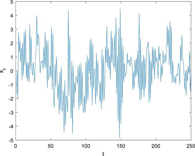
Synthetic time series with ARMA (2, 3) model.

This synthetic time series is used as input for the reversible jump MCMC algorithm. The algorithm runs as many as 100,000 iterations with a 25,000 burn-in period. The output of the reversible jump MCMC algorithm is a parameter estimation for the synthetic time series model. The histogram of order p for the synthetic ARMA model is presented in Figure 2.

Figure 2

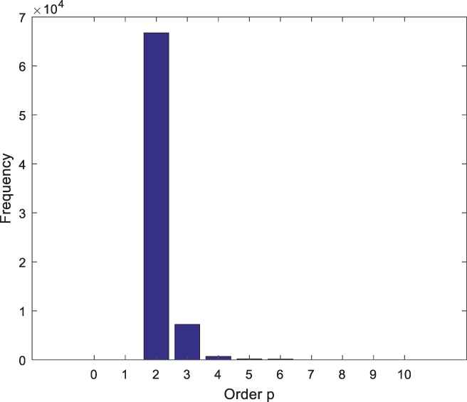
Histogram for order p of the synthetic ARMA (2, 3) model.

Figure 2 shows that the maximum order of p is reached at value 2. This histogram shows that the order estimate for p is p^=2. Also, the histogram of order q for the synthetic ARMA model is presented in Figure 3.

Figure 3

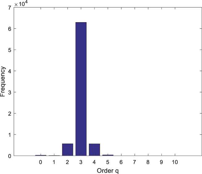
Histogram for order q of the synthetic ARMA (2, 3) model.

Figure 3 shows that the maximal order of q is reached at value 3. This histogram shows that the order estimation for q is q^=3. Given the values p^=2 and q^=3, the estimation of the ARMA (2, 3) model coefficients are presented in Table 2. The estimation of noise variance is also shown in Table 2.

p^,q^ ϕ^(2) θ^(3) β^
(2, 3) (0.25300.5732) (0.32670.33720.3765) 1.0058
Table 2

Estimation of the parameter for the ARMA (2, 3) model.

If Table 2 is compared with Table 1, the parameter estimation of the ARMA model approaches the actual parameter value.

4.2. Second Simulation

Other one-synthetic time series is made using Equation (2). The length of this time series is also 250, but the parameters are different. The parameters of the ARMA model are presented in Table 3

(p,q) ϕ(4) θ(2) β
(4, 2) (1.47731.15301.45500.9752) (0.52660.2662) 1
Table 3

The parameter value for synthetic ARMA (4, 2).

In this second simulation, the parameters of synthetic ARMA model are taken differently. Synthetic ARMA (4, 2) time series data are presented in Figure 4. This synthetic time series data contains noise that also has a Laplace distribution.

Figure 4

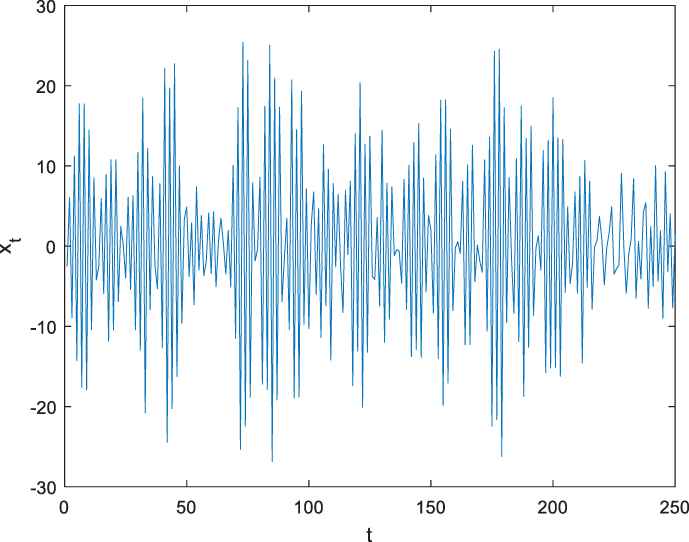
Synthetic time series with ARMA (4, 2) model.

This synthetic time series is used as input for the reversible jump MCMC algorithm. The algorithm runs as many as 100,000 iterations with a 25,000 burn-in period. The output of the reversible jump MCMC algorithm is a parameter estimation for the synthetic time series model. The histogram of order p for the synthetic ARMA model is presented in Figure 5.

Figure 5

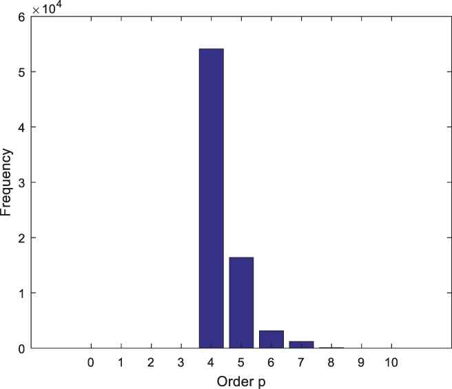
Histogram for order p of the synthetic ARMA (4, 2) model.

Figure 5 shows that the maximum order of p is reached at 4. This histogram shows that the order estimate for p is p^=4. Also, the histogram of order q for the synthetic ARMA model is presented in Figure 6.

Figure 6

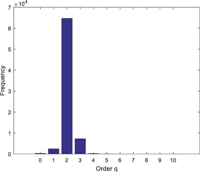
Histogram for order q of the synthetic ARMA (4, 2) model.

Figure 6 shows that the maximal order of q is reached at value 2. This histogram shows that the order estimation for q is q^=2. Given the value of p^=4 and q^=2, the estimation of the ARMA (4, 2) model coefficients are presented in Table 4. The estimation of noise variance is also shown in Table 4.

p^,q^ ϕ^(4) θ^(2) β^
(4, 2) (1.43931.10331.41930.9323) (0.51460.2518) 1.1015
Table 4

Estimation of the parameter for the ARMA (4, 2) model.

If Table 4 is compared with Table 3, the parameter estimation of the ARMA model approaches the actual parameter value. The first simulation and the second simulation show that the reversible jump MCMC algorithm can estimate the parameter of the ARMA model correctly.

If the underlying model is wrong will produce a biased estimator. So that the ARMA model is not suitable for modeling data. There is a way to identify whether the wrong model is chosen in the following way. The model is used to predict nth data based on previous n1 data. Then, the difference between the nth data forecast value and the nth data value is calculated. If the difference is relatively small, the model chosen is correct. Conversely, if the difference is large, the chosen model is wrong.

5. CONCLUSION

This paper is an effort to develop a stationary and invertible ARMA model by assuming that noise has a Laplacian distribution. The ARMA model can be used to describe future behavior only if the ARMA model is stationary. The ARMA can be used to forecast the future values of the dependent variable only if the ARMA model is invertible. Identification of ARMA model orders, estimation of ARMA model coefficients, and estimation of noise variance carried out simultaneously in the Bayesian framework. The Bayes estimator is determined using the MCMC reversible jump algorithm. The performance of reversible jump MCMC is validated in the simulations. The simulation shows that the reversible jump MCMC algorithm can estimate the parameters of the ARMA model correctly.

ACKNOWLEDGMENTS

The author would like to thank to the Ahmad Dahlan University (Indonesia) in providing grant to publish this paper. Also, the author would like to thank the reviewers who commented on improving the quality of this paper. Not to forget, the author would like to thank Professor A. Salhi, Essex University (UK).

REFERENCES

Journal
International Journal of Computational Intelligence Systems
Volume-Issue
13 - 1
Pages
310 - 317
Publication Date
2020/03/18
ISSN (Online)
1875-6883
ISSN (Print)
1875-6891
DOI
10.2991/ijcis.d.200310.006How to use a DOI?
Copyright
© 2020 The Authors. Published by Atlantis Press SARL.
Open Access
This is an open access article distributed under the CC BY-NC 4.0 license (http://creativecommons.org/licenses/by-nc/4.0/).

Cite this article

TY  - JOUR
AU  - Suparman
PY  - 2020
DA  - 2020/03/18
TI  - Hierarchical Bayesian Choice of Laplacian ARMA Models Based on Reversible Jump MCMC Computation
JO  - International Journal of Computational Intelligence Systems
SP  - 310
EP  - 317
VL  - 13
IS  - 1
SN  - 1875-6883
UR  - https://doi.org/10.2991/ijcis.d.200310.006
DO  - 10.2991/ijcis.d.200310.006
ID  - 2020
ER  -