
Multi-Sine Cosine Algorithm for Solving Nonlinear Bilevel Programming Problems
- DOI
- 10.2991/ijcis.d.200411.001How to use a DOI?
- Keywords
- Nonlinear bilevel programming problems; Sine cosine algorithm; Optimization
- Abstract
In this paper, multi-sine cosine algorithm (MSCA) is presented to solve nonlinear bilevel programming problems (NBLPPs); where three different populations (completely separate from one another) of sine cosine algorithm (SCA) are used. The first population is used to solve the upper level problem, while the second one is used to solve the lower level problem. In addition, the Kuhn–Tucker conditions are used to transform the bilevel programming problem to constrained optimization problem. This constrained optimization problem is solved by the third population of SCA and if the objective function value equal to zero, the obtained solution from solving the upper and lower levels is feasible. The heuristic algorithm didn't used only to get the feasible solution because this requires a lot of time and efforts, so we used Kuhn–Tucker conditions to get the feasible solution quickly. Finally, the computational experiments using 14 benchmark problems, taken from the literature demonstrate the effectiveness of the proposed algorithm to solve NBLPPs.
- Copyright
- © 2020 The Authors. Published by Atlantis Press SARL.
- Open Access
- This is an open access article distributed under the CC BY-NC 4.0 license (http://creativecommons.org/licenses/by-nc/4.0/).
1. INTRODUCTION
Many practical problems such as engineering design, management, economic policy and traffic problems, can be formulated as nonlinear bilevel programming problems (NBLPP). So, it has been studied and received increasing attention in the literatures. The NBLPP is a nested optimization problem with two levels (namely the upper and lower level) in a hierarchy order. The decision maker at the upper level (the leader) firstly optimizes his/her objective function independently. After the leader picks his/her decision, the decision maker at the lower level (the follower) makes his/her decision. The leader knows the objective and constraints of the follower who may be known or not the objective and (or) constraints of the leader. However, the leaders' decision is directly influenced by the decision of the follower. Throughout the most recent decades, some surveys and bibliographic reviews were given by several authors in [1–3]. In addition, reference books on NBLPPs and related issues have emerged in [4,5].
Figure 1 show that the general structure of NBLPP involving the interlinked optimization and decision-making tasks at both levels. from the figure we can see that for any given upper level decision vector, there is a corresponding lower level optimization problem must be solved which provides the rational optimal (response) of the follower for the leader's decision [6].

General sketch of a bilevel problem.
The NLBPP is a nonconvex problem, which is extremely difficult to solve. Firstly, Jeroslow [7] pointed out to that, then Ben-Ayed and Blair [8] and Bard [9] proved sequentially that the bilevel programming problem is a NP-Hard problem. Also, Vicente et al. [10] showed that even the search for the local optima to the nonlinear bilevel programming is NP-Hard operation. For more detailed discussion of the complexity issues in bilevel programming problem (see [11]). Therefore, many researchers devote their efforts to developing algorithms for solving NLBPP.
Traditional methods for solving NBLPPs can be classified to the following categories [6]: Branch-and-bound method, decent approach, approaches based on Kuhn–Tucker conditions and penalty function approach [12]. But, the properties such as differentiation and continuity are necessary when using these traditional approaches [13,14]. In addition, the NBLPP is nonconvex, which is extremely difficult to solve by traditional methods. Thus, most of researchers tend to use the metaheuristic algorithms for solving the NBLPP because of their good characteristics such as simplicity, global search capability, implicit parallelism and overcome difficulties and limitations of traditional techniques. These methods are population-based approaches which are able to find optimal solution for large scale problems easily [15,16].
The first use of the metaheuristic algorithms to solve NBLPP was through Mathieu et al. [17]; where they developed a genetic algorithm (GA) to handle this type of problems. For the same reason, other kinds of GA were proposed for solving NBLPP in Refs. [18–24]. In addition, in Refs. [25–28], the neural network approach was used to solve NBLPP; where it can converge to the optimal solution rapidly. Furthermore, other metaheuristic algorithms are used to solve NBLPP such as tabu search [29–32], simulated annealing [33], particle swarm optimization (PSO) [34–36], fruit fly optimization algorithm [37] and evolutionary algorithms [38,39].
Sine cosine algorithm (SCA) [40], is a novel population-based optimization algorithm for solving optimization problems. Due to its efficiency and simplicity, it has gained the interest of researchers from various fields for solving optimization problems. In this paper, multi-sine cosine algorithm (MSCA) is presented for solving NBLPPs; where two populations of SCA are used to solve the upper level problem and the lower level problem. On the other hand, the Kuhn–Tucker conditions is used to convert the NBLPP to a constrained optimization problem which is solved by the third population of SCA. If the objective function value of the constrained optimization problem equal to zero, the obtained solution from solving the upper and lower levels is feasible. Many benchmark problems, taken from the literature, used to demonstrate the effectiveness of the proposed algorithm.
This paper is organized as follows: Section 2 presents the definition and properties of the bilevel programming problem. Section 3 is devoted for a brief introduction to SCA and presentation of the proposed approach. Computational experiments are introduced and discussed in Section 4. Finally, the conclusion and future works are given in Section 5.
2. DEFINITION AND PROPERTIES OF NBLPP
The NBLPPs consist of two levels, namely, the upper and lower levels each having its nonlinear objective function. NBLPPs are formulated as follows:
The constraint region (CR) of NBLPPs
The projection of CR onto the upper level's decision space
For each fixed
For each fixed
The inducible region of NBLPP
Firstly, we suppose that
To avoid situations where (7) is not well posed, it is natural to assume that
Definition 1.
A solution
Definition 2.
A feasible solution
From the definition of the feasible solution to NBLPP,
Therefore, if
Now, we can give the following definition:
Definition 3.
Denote
Obviously, the smaller the feasible weighting value is, the closer
3. THE PROPOSED ALGORITHM
3.1. Brief Introduction to Sine Cosine Algorithm
SCA [40] is a novel population-based optimization algorithm for solving optimization problems. The SCA starts with creating a multiple initial random candidate solutions. This random set is evaluated by an objective function and improved by a set of rules as any optimization technique. Then, by using a mathematical model based on the sine and cosine functions, these random solutions is moved toward the best solution. There is no guarantee of finding a solution in a single run. However, with enough number of random solutions and optimization steps (iterations), the probability of finding the global optimum increases. The SCA is used the following equation to update the positions of solutions [40].
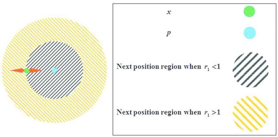
Effects of sine and cosine in Eq. (11) on the next position.
Mathematically, the steps of SCA are described as below:
Step 1. Initialization:
Initially agents are generated randomly and the parameters of SCA are stetted to form the initial population that satisfying the feasibility of the solved problem (the search domain).
Step 2. Evaluation:
For each agent, the desired optimization fitness function is evaluated.
Step 3. Setting the best position:
In the first generation, set the best position
Step 4. Updating agents positions:
The position of search agents is updated according to Eq. (11).
Step 5. Updating the best position
Determine the best agent of the current population with the best objective value. If the objective value is better than the objective value of
Step 6. Termination criteria:
If the maximum number of generations has been produced, or when the agents of the population convergences, the algorithm is terminated and the best solution obtained so far is returned as the SCA global optimum. Otherwise, Update the SCA parameters (r1, r2, r3, and r4) and go to step 2. Convergence occurs when all agents positions in the population are identical.
The steps previously described are used in the proposed algorithm: multi-SCAs to solve the NBLPPs.
3.2. The Proposed Algorithm
The idea of the proposed algorithm is to used three population of SCA, as that described previously, to solve the NBLPPs. One of them is used to solve the upper level problem, while the second is used to solve the lower level problem and the third one is used to solve the problem (9). The flow chart of the proposed algorithm is shown in Figure 3. The steps details of it are described as follows:
Step 1. Solve the upper level's problem using the first population of SCA (1) to obtain x*.
Step 2. Solve the lower level's problem using the second population of SCA (2) to obtain y*.
Step 3. By using
Step 4. Terminal conditions; where if the number of iterations is larger than the maximum number of iterations, go to Step 5, otherwise go to Step 1.
Step 5. Output the optimal solutions and output the upper level and lower level's objective function values.
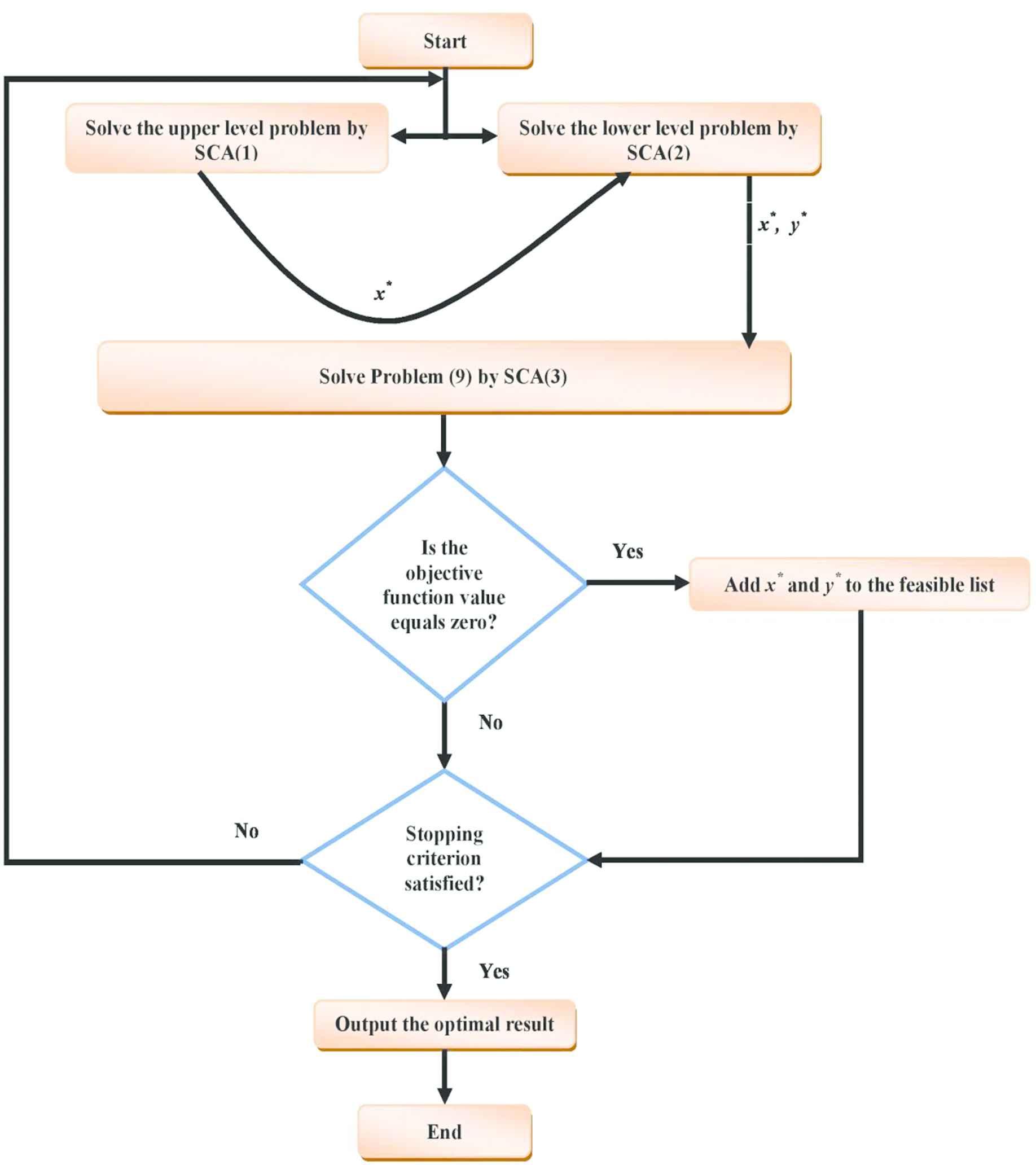
The flow chart of the proposed algorithm
The MSCA code is implemented in MATLAB, and the results are compared with previous studies, to ensure the ability of the proposed approach to solve NBLPPs. The simulations have been executed on an Intel(R) core (TM) i5 CPU M430 @ 2.27 GHz processor, installed memory (RAM): 6.00 GB. In Section 4, computational experiments are performed and their results discussed.
4. COMPUTATIONAL EXPERIMENTS
4.1. Benchmark Problems
In this section, for computational experiments, 14 benchmark problems were used to illustrate the feasibility and efficiency of the proposed algorithm for solving NBLPPs. In these problems, the properties of the upper/lower objective functions are differentiable/convex, differentiable/nonconvex, nondifferentiable/convex and nondifferentiable/nonconvex. The descriptions and details of these problems are as follows:
Problem 1:
Problem 2:
Problem 3:
Problem 4:
Problem 5:
Problem 6:
Problem 7:
Problem 8:
Problem 9:
Problem 10: the same problem 9 except
Problem 11: the same problem 9 except
Problem 12: the same problem 7 except
Problem 13: the same problem 7 except
Problem 14: the same problem 7 except
4.2. Results
The proposed algorithm was executed 50 independent runs on each of the above 14 benchmark problems. In all runs, we record the best solution found
In addition, the 14 benchmark problems have been optimized and solved, using new evolutionary algorithms (NEA), by Wang et al. [19] and the combining particle swarm optimization with chaos searching technique (PSO-CST), by Wan et al. [35]. Hence, their results are comparable with the present optimization results that obtained by MSCA.
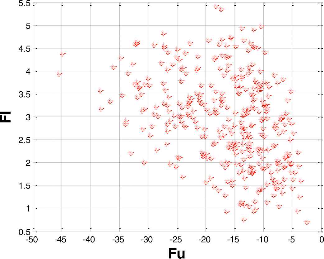
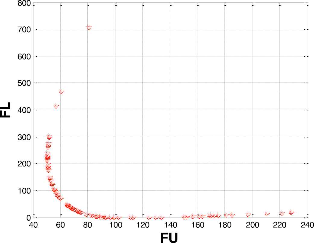
Figures 4–8 show the obtained feasible results,

The obtained feasible results,
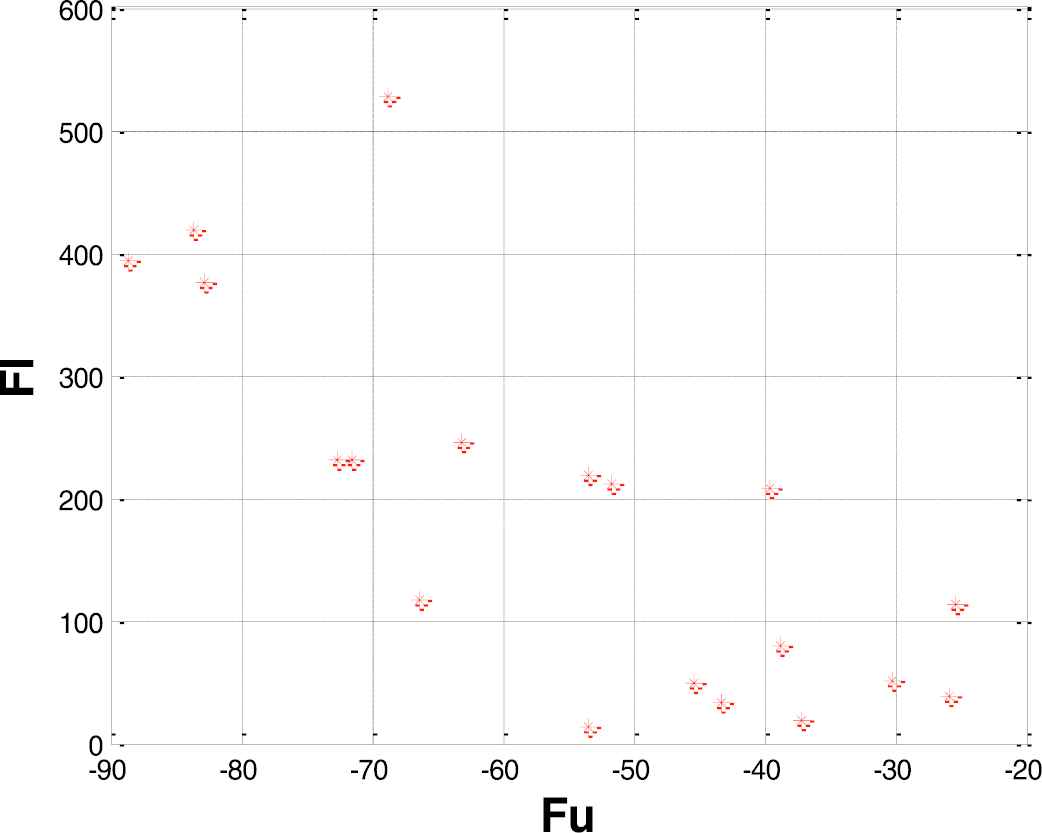
The obtained feasible results,
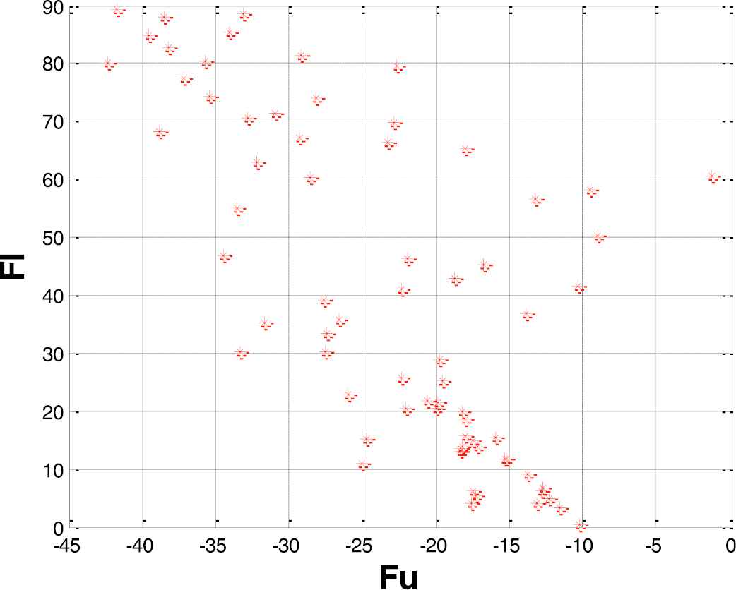
The obtained feasible results,
The obtained feasible results,
The obtained feasible results,
The comparison between the best solution
| Problem No. | NEA | PSO-CST | MSCA |
|---|---|---|---|
| 1 | (20, 5, 10, 5) | NA | (16.713, 8.286, 9.999, 4.02) |
| 2 | (0, 30, −10, 0) | NA | (19.980, 23.065, −5.733, 5.5127) |
| 3 | (4.4E-7, 2, 1.875, 0.9063) | (0.3844, 1.6124, 1.8690, 0.8041) | (0.3365, 1.0785, 1.73627, 0.56497) |
| 4 | (1.25E-13, 0.9, 0, 0.6, 0.4) | (0.1324, 0.1754, 0.6935, 0.7327, 0.2273) | (0.1885, 0.06320, 0.8608, 0.8449, 0.4560) |
| 5 | (10.0, 10.0) | (10.0020, 9.9961) | (10.0914, 9.9085) |
| 6 | (1.4E-12, 1, 7.07E-13) | (0.1511, 0.6256, 0.369) | (0.1510, 0.6256, 0.369) |
| 7 | (1.8888, 0.8889, 0) | (1.8602, 0.9073, 0.005) | (1.8602, 0.9073, 0) |
| 8 | (7.0709, 7.0713, 7.0709, 7.0703) | (7.0321, 6.842047, 5.9071, 6.8312) | (7.0321, 6.842044, 6.9071, 6.8312) |
| 9 | (20, 5, 10, 5) | (17.2024, 7.4665, 7.2189, 2.4251) | (17.2023, 7.4765, 7.2138, 2.4250) |
| 10 | (19.5629, 5.2722, 10, 5.2722) | (0.1946, 14.9870, 6.1019, 7.9628) | (0.1946, 14.9870, 6.1019, 7.9628) |
| 11 | (6.2048, 12.8594, 6.2048, 10) | (10.6084, 10.0550, 9.4545, 5.1257) | (10.6231, 10.0435, 9.3548, 5.0235) |
| 12 | (1.8888, 0.8889, 0) | (0.8606, 1.4599, 0.3138) | (0.8606, 1.4599, 0.3138) |
| 13 | (0.6648, 1.5746, 0.0721) | (0.9099, 1.5294, 0.1762) | (0.9099, 1.5294, 0.1762) |
| 14 | (0.6648, 1.5746, 0.0721) | (0.9233, 1.5083, 0.1899) | (0.9233, 1.5083, 0.1899) |
PSO, particle swarm optimization; MSCA, multi-sine cosine algorithm.
Comparison between the best solution
| Problem No. | NEA | PSO-CST | MSCA | NEA | PSO-CST | MSCA |
|---|---|---|---|---|---|---|
| 1 | 225 | NA | 194.242 | 100 | NA | 63.229 |
| 2 | 0 | NA | −25.904 | 100 | NA | 38.635 |
| 3 | −12.68 | −12.68 | −13.1380 | −1.016 | −1.016 | 0.4163 |
| 4 | −29.2 | −29.2 | −33.9402 | 3.2 | 3.2 | 2.9329 |
| 5 | 100.001 | 100.58 | 101.846 | 3.5E−11 | 0.001 | 0.008 |
| 6 | 1000 | 640.7139 | 640.71 | 1 | 0.9946 | 0.9946 |
| 7 | −1.2098 | −1.1660 | −1.0745 | 7.6168 | 7.4441 | 7.4637 |
| 8 | 1.9802 | 1.9816 | 1.9800 | −1.9802 | −1.9816 | −1.9800 |
| 9 | 0.0000 | 0.0075 | 0.0000 | 100 | 125.0854 | 124.987 |
| 10 | 6.86E−15 | 0.0000 | 0.0000 | 91.45 | 84.2367 | 84.6547 |
| 11 | 1.47E−14 | 0.0001 | 0.0000054 | 8.18 | 25.6292 | 25.6543 |
| 12 | 2.22E−16 | 0.0082 | 0.0000 | 7.62 | 2.5621 | 2.5611 |
| 13 | 1.22E−16 | 0.0374 | 0.00065 | 2.50 | 2.6969 | 2.5644 |
| 14 | 1.22E−16 | 0.0337 | 0.0000 | 2.50 | 2.7442 | 2.4446 |
PSO, particle swarm optimization; MSCA, multi-sine cosine algorithm.
Comparison between the best results,
From the Tables 1 and 2, it is clear that results obtained by MSCA are better than that obtained by NEA and PSO-CST for problems 1, 2, 4, 8, 12 and 14 for both upper level's objective function values and the lower level's objective function values. While the results of problems 11 and 13 that obtained by MSCA are only better than PSO-CST for both upper level's objective function values and the lower level's objective function values. But, the results obtained by MSCA for Problem 5 are worse than both algorithms, NEA and PSO-CST, for both upper level's objective function values and the lower level's objective function values.
For problem 3, only the upper level's objective function values that obtained by MSCA is better than that obtained by NEA and PSO-CST. For problem 6, only the upper level's objective function value that obtained by MSCA is better than that obtained by NEA and PSO-CST. For problem 7, the upper level's objective function value by MSCA is better than that obtained by NEA and PSO-CST, while the lower level's objective function value is better than PSO-CST and worse than NEA.
For problem 9, the results obtained by MSCA are better than PSO-CST for both upper level's objective function values and the lower level's objective function values. But, for comparison with NEA, MSCA succeeded only in obtaining a value for the upper level's objective function same as that obtained by NEA. Finally, for problem 10, the results obtained by MSCA are better than NEA for both upper level's objective function values and the lower level's objective function values. But, for comparison with PSO-CST, MSCA succeeded only in obtaining a value for the upper level's objective function to be same as that obtained by PSO-CST.
In general, we can say that the proposed approach MSCA was able to get better solutions for the upper level's objective function values for most benchmark problems in comparison with NEA and PSO-CST. So, the proposed algorithm MSCA is effective and efficient to solve NBLPPs.
5. CONCLUSION
This paper proposed MSCA to solve NBLPPs. Three population of sine cosine algorithm (SCA) are used. The first one is used to solve the upper level problem, while the second is used to solve the lower level problem. In addition, the bilevel programming problem is converted to a constrained optimization problem by the Kuhn–Tucker conditions. The third population of SCA is used to solve this constrained optimization problem to check the feasibility of the obtained solutions; where if the objective function value equal to zero, the obtained solution from solving the upper and lower levels is feasible. The heuristic algorithm didn't used only to get the feasible solution because this requires a lot of time and efforts, so we used Kuhn–Tucker conditions to get the feasible solution quickly. Finally, the proposed approach is tested by using 14 benchmark problems taken from the literature. The proposed approach has many features which can be concluded in many points as follows:
It has flexible adaptation to solve NBLPPs.
The solution quality is increased by using MSCA with different populations to solve the upper level problem, the lower level problem and the optimization problem that made up of transforming the bilevel programming problem using the Kuhn–Tucker conditions.
It is unlike traditional techniques; where it searches by a population of points, not single point. So, it can provide many feasible solutions for the NBLPP.
The numerical results that obtained by the computational experiments prove the superiority of the proposed algorithm, where it is better than those reported in the literature.
In our future works, we will focus on proposed other heuristic algorithms to solve NBLPP with consider other and more complex bilevel programming problems. In addition, this approach could be treating the multilevel programming problem.
CONFLICT OF INTEREST
The authors declare no conflict of interest.
AUTHORS' CONTRIBUTIONS
All authors are equally contributed in this article.
Funding Statement
The authors received no specific funding for this work.
ACKNOWLEDGMENTS
The authors would like to thank the referees for valuable remarks and suggestions that helped to increase the clarity of arguments and to improve the structure of the paper.
APPENDIX: SOME OF THE FEASIBLE SOLUTIONS FOR THE TEST PROBLEMS 1–5
| 16.4834960466894 | 8.51650395330898 | 10.0000000000000 | 2.63861763169650 | 167.338913208160 | 76.5852685972360 |
| 19.9999610471097 | 5.00003895289030 | 10.0000000000000 | 4.55420770367797 | 216.083764547691 | 100.197986446486 |
| 19.9994429763476 | 5.00055702365228 | 10.0000000000000 | 9.03645054727345 | 305.723441329499 | 116.277296371236 |
| 19.9999999997282 | 5.00000000027182 | 9.99999999999974 | 8.85599101619236 | 302.119820321134 | 114.868666709429 |
| 15.6851161584213 | 9.31488384157868 | 10.0000000000000 | 8.21240746227845 | 283.335755962416 | 33.5359999016581 |
| 18.3898918090829 | 6.61010819084000 | 10.0000000000000 | 2.85413135279575 | 171.166441921726 | 84.4976465760407 |
| 17.2385457971006 | 7.40927578297419 | 9.99999999999886 | 1.66210253238730 | 154.623100329667 | 85.4265456290013 |
| 19.2502404571777 | 5.74975954282235 | 9.99999999999992 | 4.72648563974966 | 213.156396110878 | 86.6140379963173 |
| 18.9761803650813 | 6.02381963491871 | 9.99999999999994 | 0.211221836439455 | 121.082653669293 | 114.358107113358 |
| 18.1758460986601 | 6.82415389989657 | 9.99999999999574 | 5.20000368052242 | 217.413609546716 | 69.4823233641385 |
| 15.5531318369073 | 9.43458936624393 | 9.99999999999958 | 5.78905780241159 | 236.121057629907 | 44.1271735809760 |
| 19.7401398125080 | 5.25986018749199 | 9.99999999999856 | 6.95678332015329 | 261.672119162261 | 97.7498716853925 |
| 19.0936753908462 | 5.90632460915376 | 9.99999891688560 | 9.99999993214684 | 317.579622808003 | 99.4531294631476 |
| 17.2274674197367 | 7.77253257994694 | 9.99999999999996 | 7.65973063136341 | 265.843160649615 | 52.2490095829606 |
| 19.0321290913861 | 5.96787090861395 | 10.0000000000000 | 8.17160812485705 | 280.627001602484 | 86.4358136417173 |
| 15.0000000000003 | 9.91798247504626 | 9.99999999999998 | 3.45043811219105 | 195.655839617287 | 66.8291300855036 |
| 18.9269605855044 | 6.07303941449359 | 9.99999999998792 | 7.65889278422407 | 269.750288709944 | 82.2055562056510 |
| 19.5424621286193 | 5.45753787138068 | 9.99999999999972 | 8.14708230858107 | 283.784949265316 | 98.2922327558147 |
| 16.7136534124213 | 8.28634658757844 | 9.99999999999985 | 4.02531451947929 | 194.242972301187 | 63.2295364274879 |
| 17.5060426160103 | 7.47159078123141 | 9.99999999999480 | 0.130602422568305 | 115.672057117347 | 110.230785835468 |
| 15.0002970717591 | 9.99970292824088 | 10.0000000000000 | 4.81163219552818 | 221.229673369476 | 51.9190487334729 |
| 18.6650489169518 | 6.33495108304819 | 10.0000000000000 | 8.45236251712773 | 284.261928300336 | 79.5665039143385 |
| 17.0179068399914 | 7.98209315956506 | 10.0000000000000 | 6.05130472184851 | 233.990922077486 | 52.9789604060176 |
| 15.8204430979949 | 8.50939077578589 | 9.99999999999870 | 2.86878651913862 | 190.469664663594 | 65.6939742371186 |
| 17.0530962421431 | 7.94690375775025 | 9.99999999999986 | 6.74880199335452 | 247.875485807238 | 51.1816144387828 |
| 15.0001613434793 | 8.68862772639577 | 10.0000000000000 | 8.60127598935184 | 324.967822220753 | 25.0092437867890 |
| 17.3409044097306 | 7.65909559026935 | 9.99999999999924 | 5.44569881772352 | 221.464599168172 | 58.7880028255303 |
| 18.0908751374792 | 6.90912445615208 | 9.99999999999254 | 2.01477280896775 | 153.493733675130 | 89.4169385366964 |
| 17.8848537837812 | 7.11514605258855 | 9.99999999529601 | 6.43942540281612 | 241.584737236888 | 62.6275176623175 |
| 16.9528200885189 | 8.04717991147873 | 9.99999999999988 | 5.35774689802051 | 220.253749671525 | 55.5747571171931 |
| 18.1923817058604 | 6.80761829413955 | 10.0000000000000 | 8.44690329813828 | 282.396850815986 | 69.8023733388520 |
The set of feasible solutions obtained by multi-sine cosine algorithm (MSCA) for test problem 1.
| 15.5387897122692 | 38.1450436155856 | −9.15491945801839 | 4.53573422523622 | −39.6027058169920 | 207.244207857494 |
| 2.60740248477875 | 41.9509110988793 | −4.61852559060798 | 7.36809024165173 | −82.8805293574979 | 375.835577689184 |
| 0.18717823930710 | 43.8931706442540 | −6.61513244790278 | 8.26437186046296 | −83.6734168219315 | 418.438354621163 |
| 0.02680932035748 | 35.2991104178593 | −8.80039621280156 | −4.7499391602369 | −68.8443031387396 | 526.795725183233 |
| 7.07103583706055 | 19.4657433022623 | −7.31896341018606 | 0.60300138289248 | −43.3667813975830 | 32.7654643878523 |
| 19.9802129722810 | 23.0655234782115 | −5.73346216726769 | 5.51275477227811 | −25.9047110318464 | 38.6350246069557 |
| 11.7710636419019 | 6.54015612646236 | −4.25558792658300 | −7.5472083282536 | −30.2312650629096 | 50.7467568495800 |
| 12.9704706831220 | 31.3300477541001 | −3.95188862592689 | 9.30234285492468 | −53.5334405100755 | 13.5834593807383 |
| 20.9473118708197 | 8.63797495412984 | −0.44246685074850 | −0.8408886748432 | −25.4159506602448 | 112.625795432668 |
| 12.3302573925890 | 11.7445465983031 | −2.74689258714901 | −0.8786690476717 | −38.8433540516780 | 78.6513997277838 |
| 7.98626409971397 | 33.0974022387324 | −4.65476892486140 | −0.7219464089927 | −63.1605672647203 | 245.128791992776 |
| 4.48113373869799 | 30.4780537544522 | −3.31816650112116 | 1.40888620607920 | −71.5612867736927 | 231.106874658538 |
| 1.32154550037616 | 32.0495948357767 | −5.55505693513630 | 4.31855628859339 | −72.7413330296154 | 231.992520653631 |
| 4.21103920420309 | 30.8252147842564 | −5.34277831212989 | 8.14214086062079 | −66.3748014394606 | 116.321614161765 |
| 9.05459700982721 | 38.6683374581766 | −9.61705014608239 | 4.17990467127684 | −51.7079930002750 | 211.679205898914 |
| 0.07989908374101 | 11.7959341798244 | −6.05548370439718 | −3.0575269461838 | −53.4696848991508 | 218.714472812962 |
| 2.41826382733149 | 45.2397947136916 | −3.94963764352691 | 10.8150988155511 | −88.5543541284479 | 393.905962062056 |
| 11.3500250502695 | 16.9028783280638 | −5.68380781069236 | −6.3639026885098 | −37.1514047954477 | 19.4700057069557 |
| 14.6180234494580 | 39.4112881786770 | −8.26699332368971 | 13.0005953223612 | −45.3742613086918 | 49.4203046793626 |
The set of feasible solutions obtained by multi-sine cosine algorithm (MSCA) for test problem 2.
| 0.99954526995436 | 1.16948795841407 | 9.50508979688807 | 4.50002437717950 | −22.8723367936572 | 69.8447916543844 |
| 0.56918155742448 | 0.781344934570686 | 3.33349052270050 | 1.53342431098634 | −13.1380393389281 | 4.09297280062670 |
| 0.84859268806525 | 0.308810945584173 | 9.98317824524428 | 4.28011065713497 | −22.6195678942323 | 79.7035136911194 |
| 1.22954933869177 | 0.587053750521192 | 8.34396693106365 | 1.93719315666943 | −32.1688382922881 | 62.9594015158913 |
| 0.26553572538002 | 1.83795256408921 | 3.89613479114882 | 0.88518781659479 | −25.0056997989268 | 10.8949456707324 |
| 1.11557088809851 | 0.497492625214286 | 4.01676551735323 | 0.96032191814755 | −17.1318390257390 | 13.8217924434060 |
| 0.81584142820524 | 1.20434759564482 | 9.96006144854210 | 2.52523092754962 | −38.4804111860976 | 87.9078638929383 |
| 0.73651799391718 | 1.55852841371877 | 6.42547393133041 | 2.45240890593463 | −27.5170774878842 | 30.1095882232611 |
| 1.04512758235492 | 1.34049718249537 | 8.53808873750856 | 1.36062455464306 | −38.7841455235697 | 68.2804198431533 |
| 0.76202919664434 | 1.44867591530624 | 9.19990189958513 | 1.14545956671451 | −42.3642041986663 | 80.0722741214944 |
| 1.20145811040292 | 0.95697878066106 | 4.45272476459092 | 1.91156235376235 | −18.3477551770018 | 13.1559492424954 |
| 0.66285799880180 | 0.86310985389979 | 4.54786053773273 | 1.59179499005126 | −18.3318874468509 | 13.6028219735614 |
| 0.62958003973951 | 0.06523865112941 | 9.30407513153499 | 1.39385731965786 | −35.6826015698181 | 80.3892695078353 |
| 0.23228828455389 | 1.72190351617758 | 7.24846434514192 | 3.37000776229657 | −26.5857180668436 | 35.7981122455927 |
| 0.39663826579551 | 0.91513735375060 | 6.24320858120901 | 0.01107937291180 | −27.6424626149141 | 39.2369003517093 |
| 0.72177004130695 | 1.04467113399381 | 4.59129313474070 | 0.34755653828856 | −22.0393423187836 | 20.3840939427307 |
| 0.97147411543027 | 0.26025064644296 | 7.30591591805685 | 2.82913573275856 | −22.3666078317291 | 41.1182526518257 |
| 0.67499551190213 | 0.08836974125421 | 6.36099444670490 | 2.48734200098138 | −19.7361541315696 | 28.9367782282797 |
| 0.66808821967701 | 0.11114460423195 | 5.12978559415573 | 1.72193028383340 | −18.0374997126612 | 18.5977325613830 |
| 0.15866041902200 | 1.00661557603358 | 5.09921098818522 | 2.88481570224924 | −15.1396801991016 | 11.6282204479112 |
| 0.77282063698029 | 0.33724842143606 | 8.44951283743064 | 2.47910964376220 | −28.5905279541538 | 60.1932224449795 |
| 0.33657304637855 | 1.07853609436302 | 1.73627648803347 | 0.56497801480557 | −10.2289075310003 | 0.416328799967051 |
| 1.09896346774441 | 0.99338615332173 | 7.39461010372874 | 0.41435888724943 | −33.5749159797433 | 55.0239055567936 |
The set of feasible solutions obtained by multi-sine cosine algorithm (MSCA) for test problem 3.
| 0.0219789522662545 | 0.077011832938644 | 0.055711815243667 | 0.308524587820997 | 0.306776636661773 | −13.8291217483969 | 1.15379229453176 |
| 0.148067816195352 | 0.177472256740090 | 0.725271660036854 | 0.440460620052212 | 1.21053529223336 | −21.4539108873977 | 4.08981519423132 |
| 0.168021537291266 | 0.116175395218021 | 0.124084378838530 | 0.390268921459030 | 0.250747086453702 | −17.9262815680241 | 1.41621980093227 |
| 0.0123703137499864 | 0.431178847175924 | 0.363257842542576 | 0.364210321817028 | 0.505830926517453 | −16.9623831072842 | 2.61385802549634 |
| 0.843518302596460 | 0.113291096249447 | 0.581349533963859 | 0.154011416917199 | 1.38093666823368 | −16.5601160195367 | 4.56733478244378 |
| 0.414582368495294 | 0.100595800835866 | 0.541880760168823 | 0.160931470802675 | 0.321502368887112 | −9.27478741828599 | 1.96159093891275 |
| 0.127657430738104 | 0.283815821231952 | 0.491349291504876 | 0.248206081969839 | 1.04438585415068 | −14.2969122602094 | 3.52361615497808 |
| 0.0140761551525193 | 0.0583750824277646 | 0.261579199793153 | 0.366371624544478 | 0.633499007005176 | −16.4886537815584 | 2.02577515835603 |
| 0.252324479525196 | 0.0386892819302381 | 0.346189906301264 | 0.182136907727001 | 1.15726007108396 | −12.7031099321333 | 3.17254999958185 |
| 0.265697761819986 | 0.461664257911050 | 0.026670974533030 | 0.000480820231789 | 0.500389149535003 | −5.88634463548354 | 2.21695637147691 |
| 0.143699999342032 | 0.0053359195584884 | 0.161327226651221 | 0.447399856503252 | 0.411813336196394 | −20.0688823712810 | 1.58672559400627 |
| 0.518377547658868 | 0.223043952665171 | 0.559980575472251 | 0.105803815706327 | 0.978409584122738 | −10.9450648547866 | 3.58706901241326 |
| 0.632872932051398 | 0.0593690400478564 | 0.864194044803383 | 0.051786184588027 | 1.65985680231169 | −10.5545580301569 | 4.98730484616189 |
| 0.0823677222322206 | 0.0045694785637084 | 0.219563039521511 | 0.561756819476326 | 0.624143499303446 | −24.7658143102934 | 2.12111353696437 |
| 0.963324106942369 | 0.0190578149530657 | 0.601579089920769 | 0.010725389313378 | 1.19913176034682 | −10.6020503695906 | 4.01200773677629 |
| 0.143788836089682 | 0.0190012603820694 | 0.688239480740719 | 0.757643255540148 | 0.559687005304804 | −31.0178360501080 | 2.74704810374430 |
| 0.0145966468436354 | 0.569003182561170 | 0.235304544063625 | 0.457047476193431 | 0.653063889962365 | −22.3457223363260 | 3.15108281214776 |
| 0.195948136196853 | 0.0789312669982073 | 0.716872768205968 | 0.809817735748292 | 0.798362302266633 | −34.6019777237420 | 3.47722577868079 |
| 0.527145075605880 | 0.229044481651444 | 0.427678982149580 | 0.340308328500235 | 0.972132172334458 | −20.9234844322017 | 3.69748569422750 |
| 0.0365697252020392 | 0.0550243411412149 | 0.591029056011186 | 0.568475692615912 | 0.862775968845162 | −24.3386705221536 | 3.03167509380189 |
| 0.188572921721599 | 0.0632043643092972 | 0.860849632739098 | 0.844946184511238 | 0.456092038627976 | −33.9402178350150 | 2.93296154484648 |
| 0.400626069464438 | 0.187323838293649 | 0.786531748282482 | 0.451499811431901 | 1.20041765317899 | −23.6698399857522 | 4.41414061212409 |
| 0.236480219662212 | 0.169131522541224 | 0.172408285000627 | 0.266531515364797 | 0.0235352068949085 | −12.6341361496316 | 1.06075347889990 |
| 0.357820606982177 | 0.483245276098604 | 0.0894287179525100 | 0.260795908343957 | 0.341761206418330 | −16.2367122478734 | 2.35805819831251 |
| 0.130841683032999 | 0.146346235320911 | 0.770780343077803 | 0.479208757894081 | 0.883711805134506 | −21.2521945695377 | 3.44094686491572 |
The set of feasible solutions obtained by multi-sine cosine algorithm (MSCA) for test problem 4.
| 4.54434711375526 | 4.54431459818833 | 50.4155938938367 | 267.879464464703 |
| 9.93189321542748 | 9.93189017160819 | 98.6471417913780 | 0.04174929463726 |
| 4.84160820966831 | 4.84160789016214 | 50.0501792147651 | 239.481072540709 |
| 13.5573439330933 | 6.44265606598530 | 196.456270385054 | 12.6546958714265 |
| 7.76503492696258 | 7.76503032586637 | 65.2908568612458 | 44.9557432988312 |
| 12.8977790812233 | 7.10221469600974 | 174.749864896063 | 8.39719573254597 |
| 9.19849039252296 | 9.19847563899968 | 85.2546668026141 | 5.78190075986046 |
| 4.95455549576239 | 4.95455508606452 | 50.0041345401467 | 229.108617013369 |
| 12.0700032264420 | 7.92999389563460 | 149.969903158429 | 4.28493718675652 |
| 5.41720241899285 | 5.41719191379270 | 50.3482120033490 | 189.018880735276 |
| 8.05159577927594 | 8.05158458834688 | 68.6245172092216 | 34.1667727199599 |
| 11.0902067092904 | 8.90978707056004 | 124.181249086307 | 1.18857779413173 |
| 9.06993556756303 | 9.06992747622094 | 83.1287660992336 | 7.78526894225452 |
| 5.96728465772724 | 5.96728285202540 | 51.8712937819153 | 146.365224668810 |
| 5.11983492087859 | 5.11980061967912 | 50.0290556087321 | 214.346109546181 |
| 14.2557531911277 | 5.74422783887468 | 221.338095733756 | 18.1117581517450 |
| 12.1273766665743 | 7.87261159343451 | 151.599046245361 | 4.52583138356921 |
| 5.49721908525848 | 5.49721736933950 | 50.4944690903080 | 182.475416412343 |
| 5.02239346585321 | 5.02239236113826 | 50.0010139322998 | 222.989167265069 |
| 12.4456383902228 | 7.55430870753585 | 160.875320838222 | 5.98166466593585 |
| 4.17896823484413 | 4.17896272455500 | 51.3482504699564 | 304.960082205521 |
| 6.96583456382562 | 6.96580876405524 | 57.7291676268717 | 82.8563784185986 |
| 12.7371684550677 | 7.26282840324340 | 169.727568602862 | 7.49212554878433 |
| 7.89532648981604 | 7.89527810624009 | 66.7660346308632 | 39.8680772491621 |
| 12.8152978766264 | 7.18468857158428 | 172.157838105634 | 7.92605474416644 |
| 14.4263399738156 | 5.57362048994727 | 227.712120607124 | 19.5931855733581 |
| 6.31551130053454 | 6.31550686996195 | 53.4611726124771 | 122.179308681212 |
| 10.5193213529967 | 9.48066709657031 | 110.925828392197 | 0.26971866175790 |
| 8.13431855516288 | 8.13431821981965 | 69.6479068617641 | 31.3269127902098 |
| 5.27988668172122 | 5.27984871830056 | 50.1570314939460 | 200.517377942069 |
| 5.41219412384739 | 5.41219384803432 | 50.3398105222224 | 189.431679999866 |
| 10.0914679984401 | 9.90853033524031 | 101.846093063112 | 0.00836700440941 |
The set of feasible solutions obtained by multi-sine cosine algorithm (MSCA) for test problem 5.
REFERENCES
Cite this article
TY  - JOUR
AU  - Yousria Abo-Elnaga
AU  - M.A. El-Shorbagy
PY  - 2020
DA  - 2020/04/24
TI  - Multi-Sine Cosine Algorithm for Solving Nonlinear Bilevel Programming Problems
JO  - International Journal of Computational Intelligence Systems
SP  - 421
EP  - 432
VL  - 13
IS  - 1
SN  - 1875-6883
UR  - https://doi.org/10.2991/ijcis.d.200411.001
DO  - 10.2991/ijcis.d.200411.001
ID  - Abo-Elnaga2020
ER  -