
Using Fuzzy Logic Algorithms and Growing Hierarchical Self-Organizing Maps to Define Efficient Security Inspection Strategies in a Container Terminal
 , Ventura Pérez2, Pablo Cortés1, *,
 - DOI
- 10.2991/ijcis.d.200430.001How to use a DOI?
- Keywords
- Container terminal; Port: Security inspection; Fuzzy logic; Growing hierarchical self-organizing map
- Abstract
Maritime transport is one of the oldest methods of moving various types of goods, and it continues to have an important role in our modern society. More than 20 million containers are transported across the oceans daily. However, this form of transportation is constantly threatened by illegal operations, such as the smuggling of goods or people and merchandise theft. Port security departments must be prepared to face the different threats and challenges that accompany the use of innovative techniques and devices to achieve efficient inspection strategies. Two inspection strategies are presented in this study. The first strategy is based on fuzzy logic (FL), and the second strategy is based on the growing hierarchical self-organizing map (GHSOM) approach. The weight variation and security index (SI) of a container and the readings from certain technologies, such as radio-frequency identification (RFID) and X-ray scanning, are considered as the input data. To minimize the inspection time and considering the costs associated with the security inspections of containers, the results of both inspection strategies are compared and analyzed. The findings indicate there is potential for improving the effectiveness of security inspections by employing both techniques, and the specific relevance in the case of GHSOMs is discussed.
- Copyright
- © 2020 The Authors. Published by Atlantis Press SARL.
- Open Access
- This is an open access article distributed under the CC BY-NC 4.0 license (http://creativecommons.org/licenses/by-nc/4.0/).
1. INTRODUCTION
Container transport has an important role in global supply chains and has become increasingly important around the world by contributing to economic development. However, considerable security vulnerabilities have emerged [1].
A container terminal is a complicated system with several interrelated components and different interconnected operations, such as security inspections, which should be harmoniously executed to avoid delays in the corresponding inspection times.
Security inspections can add costs, delays and uncertainties during the transport process. The disruptions in the supply chain caused by delays in the inspection area of a container terminal can be disastrous and have cascading consequences [1]. In addition, container transport can be used for illegal operations, such as the smuggling of goods and people, and can be employed by terrorist organizations to transport weapons of mass destruction or biohazards [2].
Port authorities are increasingly making demands regarding the data required for containers as they provide information about their content, country of originand shipping company. The daily analysis of container data can be a difficult process; thus, the following scientific question should be answered: Is it possible to reduce the number of containers assigned to manual inspection in ports and simultaneously improve the systems for the detection of containers that transport illegal material via new technologies without increasing the cost or time spent on inspection?
As a hypothesis based on this question, we propose that the use of artificial intelligence techniques, which have not yet been incorporated into the security inspection systems of container port terminals, can improve the process efficiency and possibly reduce or at least maintain the corresponding time and cost. Thus, the goal of this investigation is to demonstrate the possibility of increasing the detection of illegal containers (containers with illegal material or containers whose merchandise has been stolen) without increasing the cost or time of the inspection processes. The fusion of information and computational algorithms will enable the automatic identification of threats and the presentation of the relevant data to an operator to provide decision support regarding the classification of containers.
Methodologies that are based on artificial intelligence (fuzzy logic (FL) and the growing hierarchical self-organizing map (GHSOM)) and the extensive information associated with containers and their processes, including information from the technological devices that are currently used in their surveillance, are employed to develop tools for decision-making that automate the process and minimize manual inspections without reducing their reliability.
In addition, the use of the container weight as an additional decision variable in the early stages of the container inspection process is a novel proposal that arises from the new regulations that have been promoted by the International Maritime Organization (IMO) since 2016 as part of the new implemented measures for the verification of the gross mass of full containers in the Safety of Life at Sea (SOLAS) convention. These measures have been put in place due to the numerous container ship accidents caused by the excessive weight of containers. Consequently, this information could be appropriately integrated into the inspection strategy in the near future.
In this way, two new inspection strategies are developed based on FL and GHSOM methods. In our case, these strategies employ the container information along with the innovative use of the weight readings (which are currently not incorporated into security procedures) and container security indices (SIs) as well as radio-frequency identification (RFID) and nonintrusive technologies.
There is some scientific literature that deals with RFID technology [3], the SI of containers and nonintrusive inspection techniques for containers (e.g. see the English and Zuver [4]). However, the integration of these elements in one approach has not been addressed. In addition, the consideration of the FL and GHSOM approaches is novel in the scientific literature regarding their application to container inspection at ports.
The structure of the paper is as follows: A literature review of the related studies is presented in Section 2. Section 3 presents a general inspection strategy, and Section 4 details the FL and GHSOM methods. The procedures for generating the experimental data are explained in Section 5, and the results of both models are presented in Section 6. In Section 7, the discussion and final conclusions are provided.
2. LITERATURE REVIEW
The process by which security inspections are performed in container terminals is important because this process affects both the maritime supply chain and the associated costs. In this section, a scientific literature review of the inspection processes in container port terminals and the FL and GHSOM approaches is presented.
2.1. Container Inspection in Port Terminals
Among the different operations performed in a container terminal, the security inspection is one of the most important operations. The delays in the inspection area of a container terminal are primarily attributed to the manual inspection of containers. As these manual inspections require several hours per container, the manual inspection of all the containers is not viable in terms of the general efficiency of container terminal operations. Classifying the containers using a certain inspection strategy helps to reduce the number of containers that will be manually inspected, thereby reducing the time of the operations in the container terminal. By investigating different algorithms, methods and approaches, as well as the implementation of FL, we were able to improve the classification of containers and minimize the inspection times and costs.
Bakshi et al. [5] analyzed the impact of two important inspection initiatives: the Container Security Initiative (CSI) and the Security Freight Initiative (SFI). Boros et al. [6] developed a linear decision tree model to obtain the optimum sequences of inspection strategies. Boros et al. [7] considered a combination of decision trees and inspection systems by enumerating efficient inspection policies. Longo [8] designed operationally effective practices and policies to improve the flow of containers both toward the inspection zone and within the normal operations of a container terminal. Lee et al. [9] presented a genetic algorithm for optimizing the percentage of containers that are examined and the sequence of the container movements, which minimizes time-delay costs. Harris et al. [10] performed simulations to determine the necessary inspection resources for minimizing the interruption caused by an increase in security inspections in a container terminal.
Elsayed et al. [11] presented several optimization approaches to simultaneously determine the optimal levels of the sensor threshold and the sequence of the inspection. Young et al. [12] presented a study that corresponds to an extension of the study by Elsayed et al. [11], in which, unlike the latter, they present a multiobjective optimization approach for determining the optimal management of sensors and their threshold levels, considering the total costs. van Weele and Ramirez-Marquez [13] presented an optimization technique for developing an inspection strategy that establishes an inspection rate of suspect containers that minimizes the inspection costs. Riahi et al. [14] employed a dataset to establish the values of the reliability percentages, both for the country of origin and the shippers and container terminals; they obtain the SIs of the containers.
Ramirez-Marquez [15] presented an inspection strategy that introduces different types of reliability and cost measures. An evolutionary optimization approach that is known as a probabilistic solution discovery algorithm is applied to generate an optimal inspection strategy.
Concho and Ramirez-Marquez [16] developed a holistic evolutionary algorithm for identifying the optimal threshold values for every sensor and the optimal configuration for the inspection strategy. Ma et al. [17] employed the maximum likelihood (ML) estimation method to identify the efficiency factors for inspection, which improves the quarantine and clearance processes of the containers in a port. Wang et al. [18] developed a stylized queueing model with novel features related to the security checkpoints to analyze policy initiatives. Wang et al. [19] discussed an inspection investment planning problem for the international container terminal at the Dalian Port using a simulation method. They proposed a framework that combines an arena-based simulation model that considers various types of container ships and flexible container truck scheduling and routing.
Table 1 presents a summary of the investigations regarding the optimization methods for improving the security of a container terminal.
| Reference | Modeling (Algorithms) | Experimental Data Size | Main Contribution |
|---|---|---|---|
| [5] | Simulation models | Two container terminals | Effect of inspections on the flow of containers |
| [6] | Algorithms Mathematical models |
Container inspections in container terminals | Minimize the inspection costs and inspection error rate |
| [5] | Decision trees Dynamic programming algorithms |
Port inspections represented by decision trees | Establish some effective properties for inspection systems, which minimize the cost |
| [16] | Holistic evolutionary algorithmGeneral decision tree model | Container inspection strategy | Minimize the total cost of inspection while maintaining a user-specified detection rate for “suspicious” containers |
| [11] | Port-of-entry problem | Small number of inspection stations | Optimal sensor threshold levels |
| [10] | Process model Triangular distribution Simulations Sensitivity analysis |
Alabama Container Terminal | Minimize the interruptions from the increased security inspections of containers in a terminal |
| [9] | Genetic algorithm | Operations of a container terminal | Optimize the inspection process and the sequence of the movements of containers in the yard; minimize the total costs |
| [8] | Simulation models Design of experimental techniques Variance analysis |
Container terminal | Integration of the security procedures in the normal operations of the container terminal |
| [17] | Factor conception model Structural equation model |
Inspection and quarantine clearance efficiency in Shanghai, China | Provide a theoretical basis for the analysis of the internal economic effectiveness |
| [15] | (n + 1)-echelon decision tree General decision tree model |
Container inspections in container terminals | Minimizes the total cost of inspection while maintaining a user-specified detection rate for “suspicious” containers |
| [14] | Bayesian network (BN) Analytic hierarchy process (AHP) |
Case study | Evaluate the security score of a container |
| [20] | Genetic algorithms Decision tree |
Modeling of security inspections with four types of sensors | Inspection rates for suspicious containers |
| [18] | Queueing model with novel features | Security-check waiting lines for screening cargo containers | Provide a modeling framework to understand the economic trade-offs embedded in the container-inspection decisions |
| [19] | Arena-based simulation model Visual Basic for Applications Simulation experiments |
International container terminal at Dalian Port | Address an inspection investment planning problem for the international container terminal at Dalian Port using a simulation method |
| [12] | Port-of-entry problem Multiobjective optimization Analysis of variance (ANOVA) |
They considered two suspect containers per 10,000 containers | Determine the optimal levels of sensor layouts and thresholds |
Approaches for improving the security of a container terminal.
2.2. Fuzzy Logic
FL allows us to deal with nonaccurate information by considering the data as fuzzy sets. The fuzzy sets combine different rules to define the actions. Thus, control systems based on FL are able to combine the input variables by applying groups of rules that lead to one or more output values [21].
Systems based on FL can be applied to nonlinear or partially defined problems as neural networks. However, in contrast to neural networks, FL allows for the easy implementation of expert knowledge by formalizing the sometimes ambiguous knowledge of experts. In addition, FL allows for the design of inexpensive and quick control and decision systems.
The application of an FL algorithm can be described by the following three steps:
Fuzzification, where the input values are converted to fuzzy values
Inference, which is a process based on the logic rules
Defuzzification, where the fuzzy variables are reconverted, and a decision is made
FL has been used as a tool for processing large amounts of information, in which the data can have an associated degree of partial set membership. FL methods are the main actors in some investigations of system control; in other studies, FL methods aid in decision-making.
In Starczewski [27], an efficient fuzzy logic system (FLS) that is based on triangular type-2 fuzzy sets is designed. This FLS provides a new method for reducing computational complexity in t-norm operations that is extended to triangular type-2 fuzzy sets. Motepe et al. [26] presented an FL method and experimental investigation. This study was associated with real measurements of the South African power system network. Magudeeswaran and Ravichandran [25] presented an FL-based histogram equalization (FHE) method to enhance image contrast to highlight the details of a hidden image or increase the image contrast with a new dynamic range.
Liang et al. [24] used fuzzy set theory to construct an optimum output quantity decision model to obtain the maximum profit of a duopoly market. Huerta et al. [22] presented an FL-based preprocessing approach that consists of two main steps. First, the approach employs fuzzy inference rules to transform the gene expression levels of a given dataset into fuzzy values. Second, the approach applies a similarity relation to the fuzzy values to define the fuzzy equivalence groups. Each group contains similar genes, which assists with the selection of an essential subset of genes for the classification and analysis of microarray data. Hsueh [23] used the Delphi method and FL theory to develop a quantification assessment model that is based on the qualitative analysis used to evaluate the results and influences of participation in environmental protection education and green community development by residents of the Taiwan community.
Table 2 presents a summary of the investigations regarding the FL method.
| Reference | Modeling (Algorithms) | Experimental Data Size | Main Contribution |
|---|---|---|---|
| [22] | Fuzzy logic | Analysis of microarray data | Gene selection |
| [23] | Fuzzy logic | Community residents' participation in environmental protection education | Assess the results and influences of community residents' participation in environmental protection education on green community development |
| [24] | Fuzzy decision environment | Duopoly market | Construct an optimum output quantity decision model that aims to maximize the profit of a duopoly market |
| [25] | FL-based histogram equalization | Images | Unveil the hidden image details or increase the image contrast with a new dynamic range |
| [26] | FL | South African power systems network | Determine a distribution power systems' loading measurement accuracy |
| [27] | FLS based on triangular type-2 fuzzy sets | t-norm operations | Provide a new method for computational complexity reduction in t-norm operations extended to triangular type-2 fuzzy sets |
FL, fuzzy logic; FLS, fuzzy logic system.
Approaches for fuzzy logic method.
2.3. The SOM and GHSOM
Self-organizing maps (SOMs) were developed by Teuvo Kohonen in the 1990s (see Kohonen [28] for a good introduction to SOMs) as a continuation of the competitive networks proposed by Von Der Malsburg. SOM networks have been successfully applied to a large variety of problems, such as pattern classification, size reduction, process monitoring and data mining, among others [21].
A SOM obtains the statistical characteristics of the input data which is then applied to a wide data classification field [29]. However, the effectiveness of traditional SOM models is limited by the following issues:
Problems related to their statistical topology and their inability to represent the hierarchical relationships in the input data [30–35].
The size and dimensionality of the SOM model, which is corrected prior to the training process and determined by trial and error [30–33,35,1].
The GHSOM approach seeks to overcome these problems [30–32,36,34,33,37].
The GHSOM has an adaptive architecture without supervision that focuses on clustering data. When the distribution of the data increases in a hierarchical manner, the approach allows for its hierarchical decomposition and exploration of the data clusters in a horizontal manner [38]. This self-organizing model (GHSOM) has a hierarchical architecture that is divided into layers; each layer is composed of different SOMs, and the size of each SOM is automatically determined during the unsupervised learning process [34]. The main advantage of a GHSOM compared with a traditional SOM is that the trial and error are removed from the training process. An ideal topology is formed in an unsupervised manner based on the training data [33].
Palomo et al. [34] presented a new approach for analyzing and visualizing network forensics data (network forensics is an area of research that collects information regarding crimes that involve digital evidence) based on GHSOMs. Ippoliti and Zhou [33] proposed an adaptive GHSOM approach (AGHSOM) for network anomaly detection. Chattopadhyay et al. [31] proposed a GHSOM that improves the cell formation problem (CFP) of a cellular manufacturing system. Chan and Pampalk [30] developed a GHSOM Toolbox for MATLAB, which has an advantage in visualization due to its capability of presenting classes and subclasses of similar data. By combining the GHSOM with mutual information, Zhang et al. [37] proposed a new intrusion detection method for detecting unknown network attacks.
Table 3 provides a summary of investigations on the SOM and GHSOM approaches.
| Reference | Modeling (Algorithms) | Experimental Data Size | Main Contribution |
|---|---|---|---|
| [30] | GHSOM Toolbox for MATLAB | Determine the size of the SOM Presenting classes and subclasses of similar data | Development of the GHSOM Toolbox for MATLAB |
| [31] | SOM approach GHSOM | CFP of cellular manufacturing system | Development of optimum machine-part cell formation algorithms |
| [32] | GHSOM | Set of data | Grow in terms of map size and a three-dimensional tree-structure to represent the hierarchical structure in a data collection during an unsupervised training process |
| [36] | Growing hierarchical tree SOM (GHTSOM) | Set of Internet meaning data | Allow the network to adapt the topology of each layer of the hierarchy to the characteristics of the training set |
| [33] | AGHSOM | Set of online data | Network anomaly detection |
| [34] | GHSOM | Network forensics | Improve the visualization of network traffic data |
| [37] | GHSOM method | Set of data | Clustering of input data |
SOM, self-organizing maps; GHSOM, growing hierarchical self-organizing map; CFP, cell formation problem.
Approaches for SOM and GHSOM.
In Section 2.1, the different investigations within the optimization field for improving the security inspections in port terminals were analyzed. Although different models, simulations and optimization designs have been employed to achieve an optimal inspection strategy, the inspection strategies based on FL or SOM and GHSOM approaches have not been designed considering the container weights as input data, which is our research contribution. Both strategies are compared and analyzed to obtain the most efficient inspection strategy when classifying the containers as follows: suspicious containers will be manually inspected; probably suspicious containers will be inspected by X-ray scanning; and not suspicious containers will be released to continue their path through the container terminal.
3. THE INSPECTION STRATEGY
The following values were employed for this investigation: the weight variation
 |
Security percentages of the countries of origin and carriers/ports.
Safety management regulation is an important complement to market forces to establish a sufficient safety level in high-risk industries [39], which explains why the IMO implemented measures for the verification of the gross mass of full containers in the SOLAS convention [40] due to the numerous container ship accidents caused by the excessive weight of containers. The new regulation, which has been in effect since July 1, 2016, seeks to avoid accidents caused by an improper weight distribution by requiring the verification of the container weights. This information is reflected in the documentation. These regulations enable the use of the container weight as input data for our investigation; this variable has not been included in inspection strategies for decision-making.
The RFID technologies are very reliable but cannot guarantee 100% security, which indicates that an inspection strategy based on RFID technologies would not provide optimal results when classifying containers as suspicious or not suspicious. In addition to these technologies, the container weights and other technologies and indicators will be considered in this study.
The RFID technologies have the following limitations [41]:
The collisions that occur when trying to simultaneously read several tags cause data loss.
The RFID tags can be damaged during container transport.
The weather conditions can affect the RFID tag and cause the transmission of inaccurate readings regarding the opened or closed condition of the container.
The containers that are considered to be suspicious can be subjected to X-ray scanning as in the image discrimination system proposed by [42], where the theory of using two X-ray energies (
Dual-energy imaging comprises a technique that scans objects with dual X-ray energy layers,
3.1. The General Inspection Strategy
Inside a container terminal, all the containers undergo an initial inspection, the results of which are used to classify them as “suspicious” or “not suspicious.” Based on this classification, a container will be subjected to additional controls that will enable its entrance or clearance or determine whether it has to be manually inspected.
The use decision trees for inspection strategies was first suggested by Boros et al. [6], later in a more general way the process was represented as a decision tree by Van Weele and Ramirez-Marquez [20], where the results of each inspection determine the path of the container through the tree.
The decision tree models presented in this document consider different factors in the inspection process to improve the strategy, such as the weight and security score of a container and the RFID readings. The decision trees for each optimization method are shown in Figures 1 and 2.

Decision tree for the FL-based inspection strategy.
Decision tree of the GHSOM-based inspection strategy.
Both trees are similar for the inspection and classification of a container. As shown in Figure 1, the largest difference between the two strategies is that the RFID reading from the container is analyzed in node 1 to indicate if the container has been opened during transit. If the container was opened, it is classified as a suspicious container and will directly undergo manual inspection; otherwise, it will be classified as probably suspicious and will pass to node 2, where the classification of the container can be obtained by analyzing the container input data, such as the weight variation
This separation of the variables in the decision tree is attributed to the fuzzy nature of the three measures (weight variation, SI and X-ray results), which contrasts the use of the binary RFID variable.
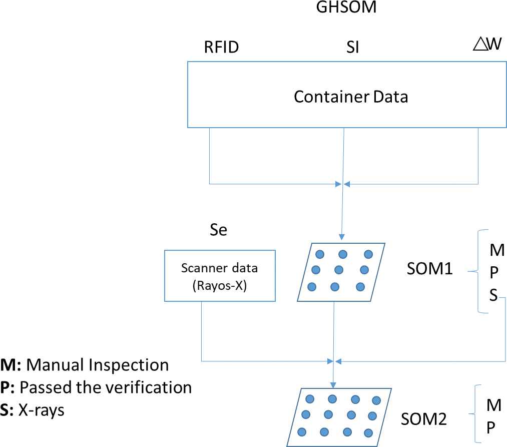
To generate the first GHSOM or SOM 1 level, the input data, which consists of the weight variation, SI values and the RFID readings, as shown in Figure 2, are simultaneously analyzed in the first step. Thus, first, the containers are classified into three sets: M, for the containers that are suspicious that will directly proceed to manual inspection; P, for containers that are not suspicious, which will leave the inspection area; and S, for the containers that will be subjected to X-ray scanning, since there is not sufficient information to determine if they are suspicious. The SOM is employed for data clustering and visualization, which enables the classification of the variables regardless of whether they are fuzzy or not.
4. DECISION SUPPORT METHODOLOGIES FOR SECURITY INSPECTION BASED ON ARTIFICIAL INTELLIGENCE
In this section, we detail the proposed methodology for security inspection strategies based on the FL and GSHOM approaches.
4.1. The FL Model
The proposed inspection strategy FL-based process is explained next.
As indicated,
We will use FL to sharpen the inspection strategy results. The input data, weight variation
4.1.1. The data and variables of the FL model
In the model of Figure 1, node 1 is a classic logic decision. If a container has been opened, it will be manually inspected. If a container has not been opened, it will proceed to node 2, where it will be classified again due to the fuzzy algorithm. The variables to be analyzed by the algorithm in nodes 2 and 3 of the decision tree are defined in the following section.
The structure followed during the decision processes starts with the statement of the input and output variables. Then, the membership functions for each input are explained, and the fuzzy linguistic variables are detailed by means of the structure rules (IF x AND y THEN z) creating the rule matrix. Finally, to solve the problem we make use of the Root-Sum-Square (RSS) method.
The calculations for all the fuzzy variables were performed using the MATLAB Fuzzy Toolbox. This toolbox allows the creation and editing of fuzzy inferences with graphical tools or command line functions; they can also be generated with the adaptive cluster techniques in the toolbox.
4.1.2. Decision process in node 2
Two fuzzy variables are defined: the weight and security score of the container:
System states
Input 1: the weight variation
The weight variation input variable,
A variation between the values above the threshold suggests that the container should be considered as suspicious. This could be due to an increase in the weight (that could be associated with adding some illegal goods for smuggling) or a decrease in the weight (that could be associated with the theft of goods from the container).
Input 2: container SI
The container SI will be
Figure 3 shows the membership function according to the weight variation and SI values and the defuzzification function for determining the output of node 2.
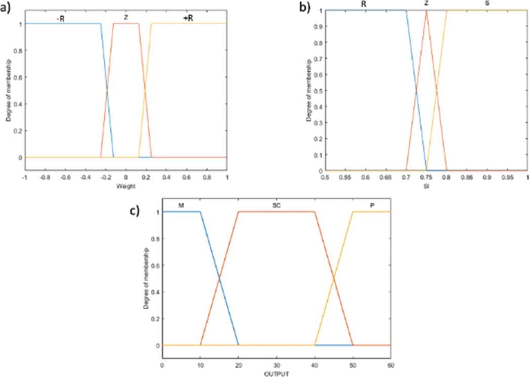
a) Membership function for the weight variation, W; b) Membership function for the SI of a container; c) Output of node 2.
Table 5 presents the matrix of rules that determines the membership.
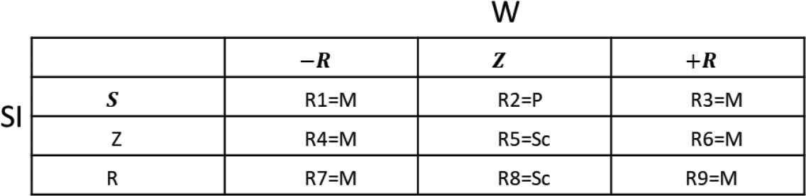 |
Rule matrix for Node 2.
Structure rules and the rule matrix
The RSS method is applied to solve the system. This approach combines the effects of all the rules, scales the functions according to their dimensions and calculates the fuzzy centroid of the composed area.
Using the RSS approach, the values of the probably suspicious containers (Sc) can be obtained using Equation (7); the values of the not suspicious containers (P) can be obtained using Equation (8); and the values of the suspicious containers (M) can be obtained using Equation (10). These equations are incorporated into the defuzzification function for the final decision (Figure 3c).
4.1.3. Decision process in node 3
After passing through node 2, all the containers that are classified as probably suspicious will be inspected by a nonintrusive X-ray scan in node 3, where they will be classified again using the
For node 3, input 1 and input 2 (the weight variation and SI of a container, respectively) will be the same as in node 2. The container will be scanned by X-ray and a new input is defined for the X-ray analysis data and the output of node 3.
where
The output will be as follows:
System states
Input 3: X-ray scanning result
The X-ray scanning result will be
Figure 4 represents the membership functions according to the values of the weight variation, SI and the X-ray scanning result. Figure 5 shows the defuzzification function for determining the output of node 3.
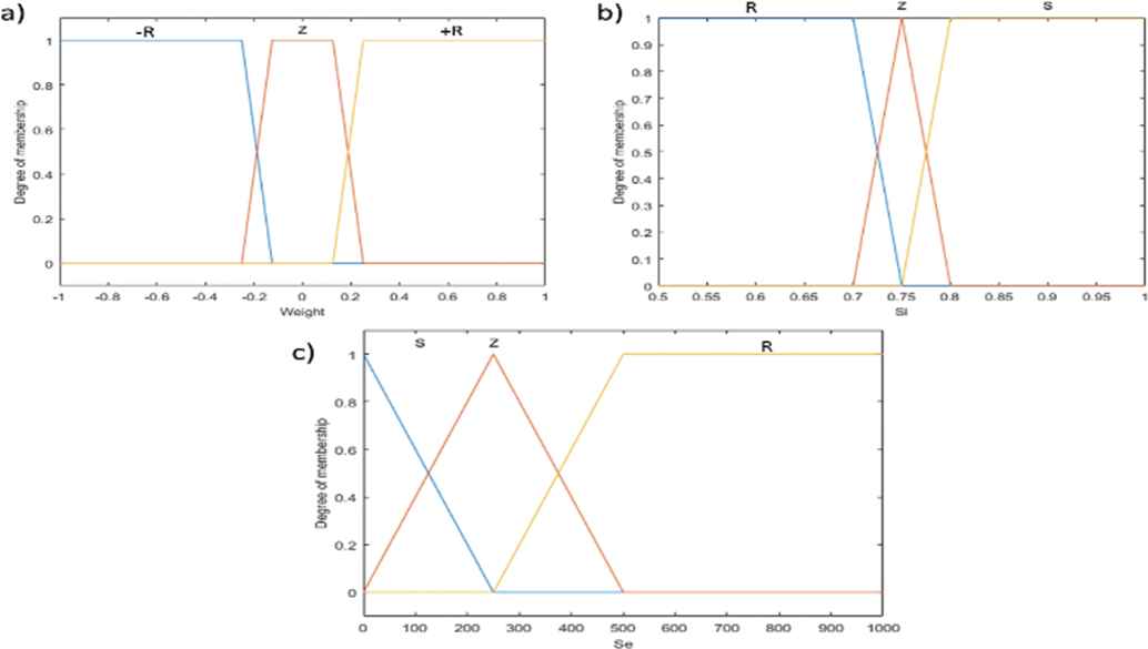
a) Membership function for the weight variation ∆W; b) Membership function for the SI of a container; c) Membership function for Se.

Output of node 3.
Table 6 presents the matrix of rules that determine the membership.
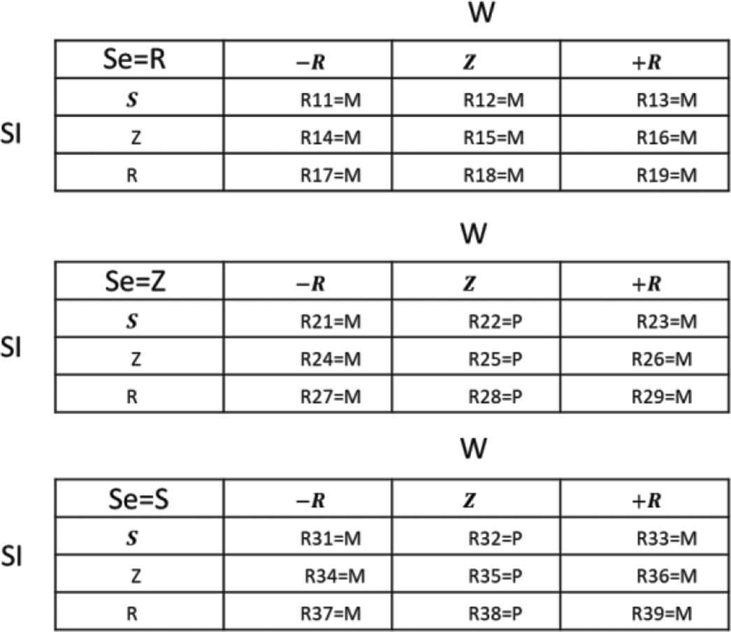 |
Structure of rules for node 3.
4.1.4. Structure rules and the rule matrix
The RSS method is applied to solve the system and obtain the values of the suspicions containers (M) in Equation (13) and not suspicious containers (P) in Equation (14), which are incorporated into the defuzzification function for the final decision (Figure 5):
4.2. The GHSOM Model
As previously explained, the GHSOM rules are networks formed by several SOM networks whose size is automatically determined during the unsupervised learning process [34]. In this section, their operation and implementation are described, beginning with the SOM network training process.
4.2.1. SOM network training
A SOM is an unsupervised neural network model that can be used for data clustering and visualization applications [44]. An SOM can project high-dimension patterns onto a low-dimension topology map. The SOM maps consist of a one-dimensional (1D) or two-dimensional (2D) node grid. These nodes are also referred to as neurons. The weight vector of each neuron has the same dimension as the input vector.
These neural networks classify the unsupervised input data, and their architecture consists of two layers: the first layer, which is also called the competition layer, consists of the learning nodes, which contain information about the resulting representation, and the input nodes, which represent the original vectors during the training process. All the elements of the first layer are connected to all the elements of the second layer.
Figure 6 shows the basic structure of an SOM network, where

Basic structure of an SOM network.
The classic SOM network learning algorithm can be formulated as follows (for an in-depth analysis of the algorithm, refer to [45]):
The synaptic weights,
Equation (15) determines the Euclidean distance between the synaptic weight vector and the input, where
The synaptic weights of the winner neuron and its neighboring neurons are actualized according to the weight actualization rules.
The learning rate determines the neuron weight variation; it is a time-decreasing function that is actualized with a linear function and its values fall between 0 and 1.
The neighborhood function is used to determine which neurons,
The neighborhood function,
The simplest representation for the neighborhood function is step-like:
A neuron is in the neighborhood of the winner neuron if the Euclidean distance is smaller than
The algorithm is repeated from step 2) to the required number of iterations,
4.2.2. GHSOM network training
In this section, we explain the procedures for training the SOM 1 and 2 networks, in which neuron identification was performed to obtain the classification results of the container. Figure 7 shows the algorithm designed to determine the size of the networks.
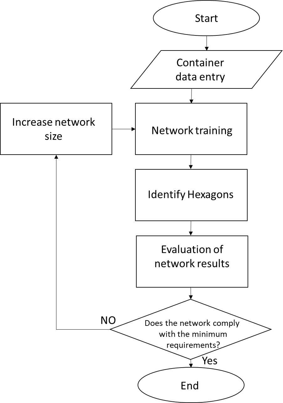
Decision algorithm for the SOM network size.
After the network has been trained and its neurons have been identified, the network is tested and evaluated, and the container data are introduced.
We used the MATLAB GHSOM Toolbox to train our network; this toolbox increases the functionality of the SOM Toolbox [30]. The use of the basic functions of the SOM Toolbox to create the GSHOM networks provides a more robust and standardized network than the SOM Toolbox. Once the network is trained, the decision algorithm identifies the hexagons to then use to evaluate the network results. If the classification error rate of the containers is less than 0.5% (which indicates that at least 50 containers have been misclassified), then the network is considered to be satisfactory; otherwise, the size of the network will be increased and retrained.
For the SOM 1 network, the algorithm determined an optimal size of 10 × 10. The algorithm determined an optimal size of 20×20 for the SOM 2 network.
SOM 1
This phase is the first step of the inspection strategy where the network classifies the input data, which consist of the weight variation, ∆W,

Trained SOM 1 network with the weights and distances of the neighboring neurons.
In Figure 8, the blue hexagons represent the neurons, the red lines connect the neighboring neurons, and the other colors represent the distances between the neurons; the darker colors represent longer distances, and the lighter colors represent shorter distances.
After properly training the neurons to achieve a container classification error rate of less than 0.5% (fewer than 50 misclassified containers), the containers that are assigned to each neuron of the SOM 1 network are identified, that is, the neurons that will classify the containers as suspicious, probably suspicions or not suspicious, depending on their information, are identified.
Figure 3a and 3b show the membership functions for the
The neuron classification in the SOM 1 network, the training of which was depicted in Figure 8, is visualized in Figure 9. The containers associated with neurons classified as

Distribution of the SOM 1 final classification.
In the following level of the GHSOM consisting of SOM 2, the ∆W,
SOM 2
With the variables ∆W,
Figure 10 shows the results of the decision algorithm that defines the size of the network (see the flow chart in Figure 7) for SOM 2, which defines a 20 × 20 network size. Again, this configuration is the final configuration that meets the error requirements stated in the algorithm to define the network size.
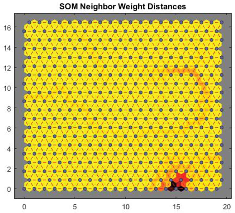
Trained SOM 2 network with the weights and distances of the neighboring neurons.
In Figure 10, the blue hexagons represent the neurons; the red lines connect the neighboring neurons, the different colors represent the distances between the neurons the darker colors represent longer distances; and the lighter colors represent shorter distances. Unlike in SOM 1, the distances between the neurons are very small due to the size of the network and the variable values.
The type of neuron that will classify the containers as suspicions or not suspicious, depending on the variables ∆W, SI, RFID and
As previously explained, to identify which type of containers are assigned to each neuron, the membership functions were employed for the ∆W and SI variables. For the new SOM 2 network, the membership functions for
Figure 11 shows the neuron positions for the container classification obtained by the algorithm, given the network size that was shown in Figure 10. The containers located in neurons classified as
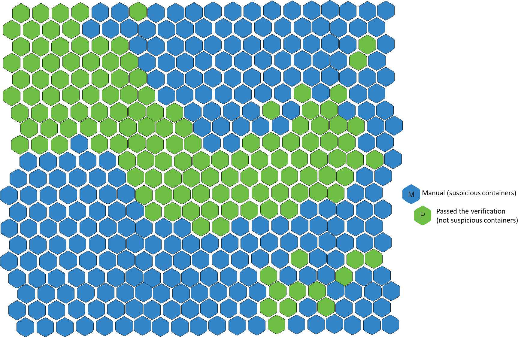
Distribution of the SOM 2 final classification.
5. ANALYSIS OF THE RESULTS
The results of each inspection strategy are analyzed in this section. Each strategy uses the same data for the 10,000 containers as input (see Annex 1 for the details related to the data generation for the experimentation). The efficiency of each strategy based on artificial intelligence is observed for the classification of containers. The ability to minimize the cost and times of the inspection zone in a container terminal and the ability to minimize the number of illegal containers that are not detected in the inspection zone are observed, as we presented in the initial scientific equation. The novel introduction of the weight variation variable, ∆W, is very useful and discriminative for the classification of the container input data since both methods can be employed to make decisions for the classification of each container.
5.1. The Base Case
The same data for 10,000 containers were used for each inspection strategy. The results of the inspection strategies, the strategy based on FL and the strategy based on GHSOM networks, are presented in the following section.
5.1.1. The FL approach
In node 1, the RFID tags of the 10,000 containers are analyzed, of which 732 containers were found to have been illegally opened and were classified as suspicious and manually inspected. Of the 732 suspicious containers, 263 containers contained some smuggled merchandise, and 469 containers had part of their merchandise stolen.
A total of 9,268 containers were classified as likely suspicious and were used as the input data of node 2. Using the
The
In node 3, 2,998 containers were analyzed and passed through an X-ray inspection. With the ∆W and
Thus, the error rate is 0.11%. A summary of the inspection strategy results is shown in Figure 12. This output error rate, for both nodes 2 and 3, is attributed to the notion that the values used to classify the containers were very small and were almost undetectable by the X-ray scan, weight variation or the SIs. This finding is observed in Figures 13 and 14, where the weight variation is given in tons

Decision tree summary of the container classification.
Classification analysis of the node 2 output.

Classification analysis of the node 3 output.
Specifically, the classification error rate of the inspection strategy was attributed to the very small values of different variables. As shown in Figure 13, two containers had high SI values and were illegal but were classified as not suspicious when a small weight variation existed between the two containers. As shown in Figure 14, these 9 containers were classified as not suspicious when they were illegal because their weight variation was very small and their SI values were very high or the values of the X-ray simulation were low; that is, if two of the container variables had values similar to those that are considered as safe, the system considered these containers not suspicious.
The inspection strategy based on FL consists of three steps: (i) the first node detects containers that were forced open as determined by the RFID data, (ii) the second node makes use of the ∆W and
5.1.2. The GHSOM approach
In SOM 1, the ∆W,
In SOM 2, 4,947 containers were analyzed and subjected to an X-ray scan. With the ∆W,
A summary of the inspection strategy results is shown in Figure 15. This error rate in the SOM 2 output is attributed to the fact that the illegal merchandise in the container was not easily detected by the X-ray scanning model, which hindered the analysis of the weight variation and
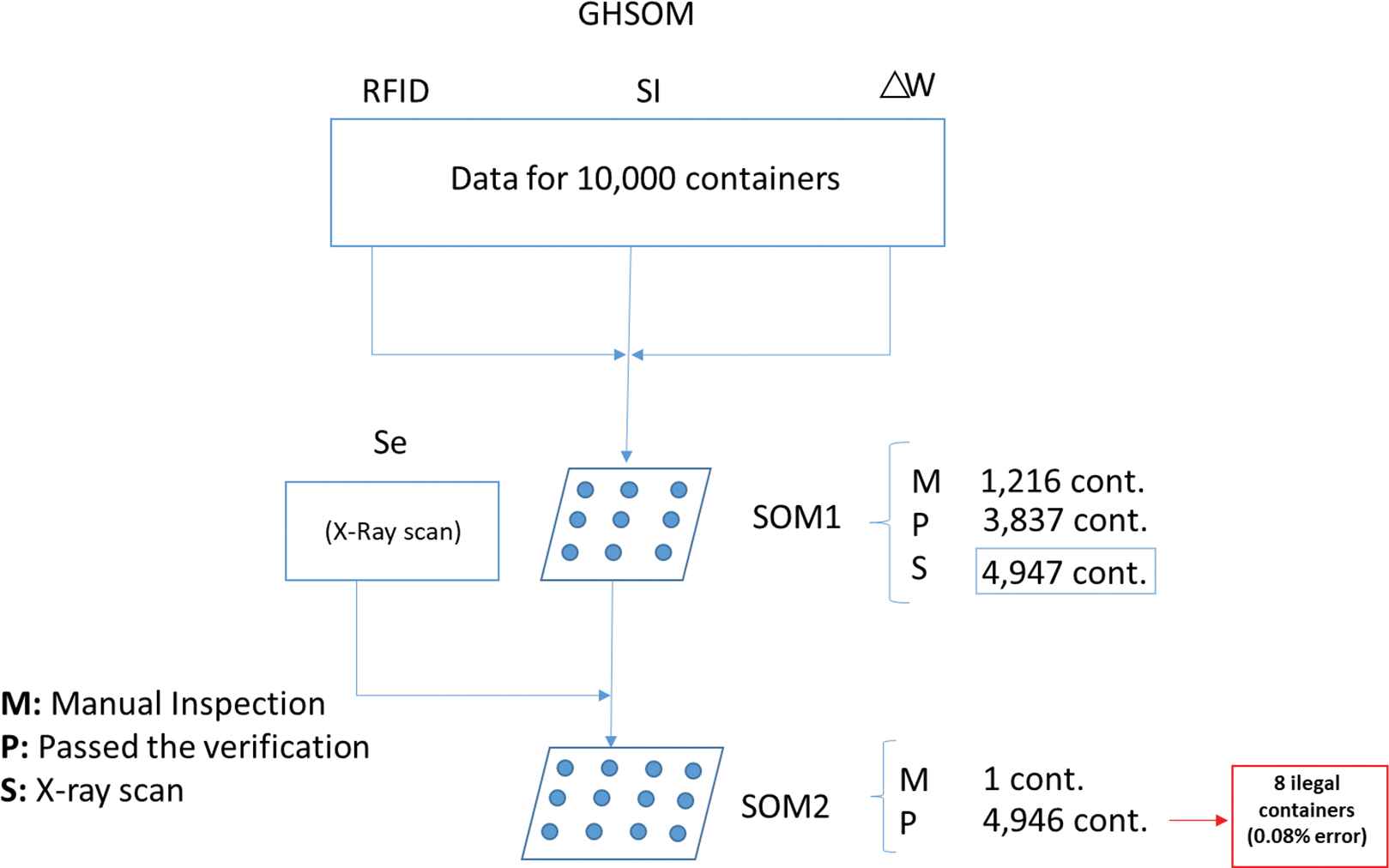
Summary of the classification of the containers.
Figure 15 shows the complete inspection strategy and the results. Note that there are no errors in the classification obtained by SOM 1 for the suspicions containers and not suspicions containers. The classification obtained by SOM 2 has an error rate of 0.08%, as the amount of illegal merchandise was not detectable by the X-ray scans in this case.
Figure 16 shows the SOM 1 output; the data are grouped into two data clouds defined by the
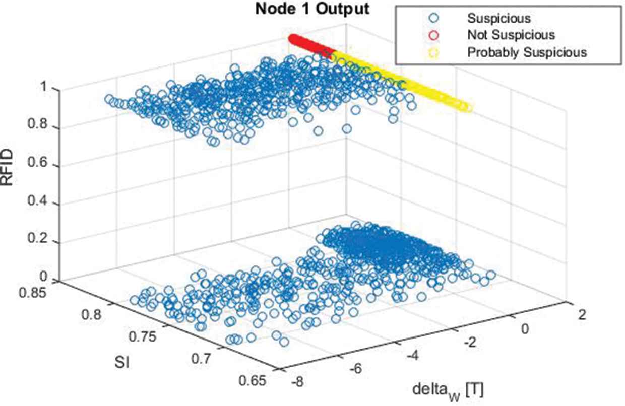
Classification analysis of the SOM 1 output.
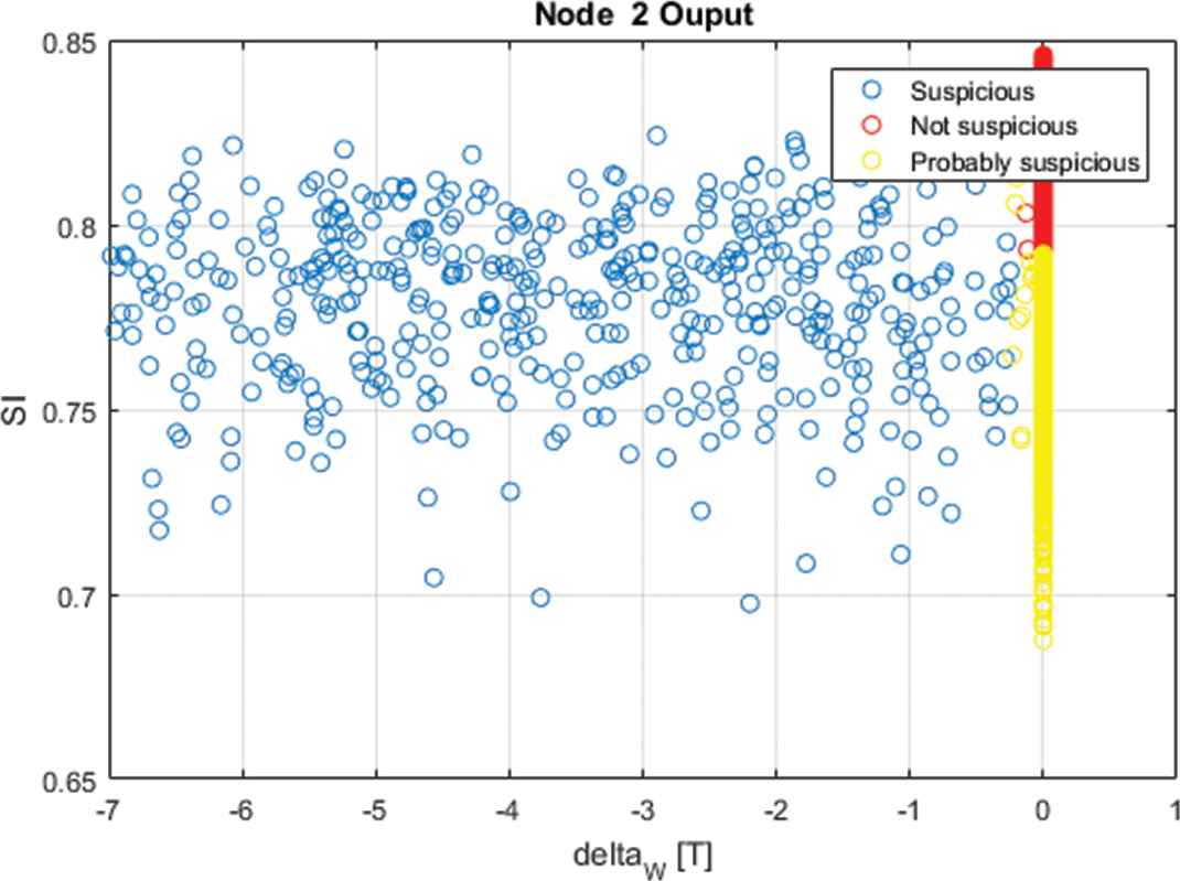
The SOM 2 output is given in Figure 17. A second analysis of the parameters was necessary to detect another suspicious container from the 8 remaining containers in this inspection strategy point. The combination of the ∆W and

Classification analysis of the SOM 2 output.
6. SUMMARY OF THE RESULTS
In this final summary, we follow a specific table design that allows us to easily visualize the performance of each approach. Each row represents the instances of the predetermined class, and each column represents the instances of the predicted class (or vice versa) [46]. Given a classifier and an instance, there are four possible results as Table 7 shows.
| Predicted Values |
|||
|---|---|---|---|
| Positive | Negative | ||
| Real values | Positive | a | b |
| Negative | c | d | |
Confusion matrix.
If the instance is positive and it is classified as positive, then it is a true positive (a). However, if it is classified as negative, it is a false negative (b). If the instance is negative and it is classified as negative, then it is a true negative (d). However, if it is classified as positive, it is a false positive (c). Given a classifier and a set of instances, a confusion matrix can be easily constructed (see [47]).
The rate of true positives and negatives, as well as false positives and negatives, can be calculated using the following metrics (21–24).
The true positive rate of the classification is given by
The false positive rate of the classification is given by
The true negative rate of the classification is given by
The false negative rate of the classification is given by
Next, the confusion matrix of the proposed algorithms allows us to analyze the performance of the FL and GHSOM approaches (see Tables 8 and 9).
| P (Passed the Verification) | M (Manual) | |
|---|---|---|
| L (legal) | 8,775 (100%) | 0 (0%) |
| I (illegal) | 11 (0.89%) | 1,214 (99.1%) |
Confusion matrix for the fuzzy logic approach.
| P (Passed the Verification) | M (Manual) | |
|---|---|---|
| L (legal) | 8,775 (100%) | 0 (0%) |
| I (illegal) | 8 (0.65%) | 1,217 (99.34%) |
GHSOM, growing hierarchical self-organizing map.
Confusion matrix for the GHSOM approach.
Fuzzy Logic
The algorithm shows a good capability to appropriately classify the different containers of our case study. All the legal containers were correctly classified in 100% of the cases and did not require any manual inspection with its corresponding cost and time. In the case of the illegal containers, the algorithm showed a very low rate of confusion. Only 11 containers representing 0.89% of the instances were classified as false positives and passed the verification without a manual inspection. Of the illegal containers, 99.1% were appropriately identified for manual inspection. Therefore, the algorithm presents a low failure rate.
GHSOM
Regarding the GHSOM approach, the algorithm shows a very high degree of appropriate classification. First, all the legal containers were correctly classified in 100% of the cases and did not require manual inspection with its corresponding cost and time. Regarding the false negative containers, only 8 containers (0.65%) were inadequately classified and were not subjected to manual inspection. On the other hand, 1,217 illegal containers were appropriately subjected to manual inspection.
The comparison of the approaches shows that both of the algorithms are very good classifiers that perfectly classify the legal containers. Both approaches show a very good level of classification for illegal containers with a very low error rate. In this line, the GSHOM approach showed a slightly better performance.
7. CONCLUSIONS
This study has demonstrated how efficient security inspections can be achieved by increasing the security of container transport and minimizing the time and cost spent by applying two artificial intelligence methodologies, which are based on FL and the GHSOM. The container input data, such as the RFID readings, X-ray scanning results and container security data, were analyzed. A novel contribution of the new IMO regulations was the inclusion of the container weight variation to achieve a better adjusted classification of the containers and reduce the number of suspicious containers that are not detected in the inspection area.
Additionally, the weight sensors in the container terminal work with threshold values between 40 and 20 tons. The sensors recommended in the OIMLR 60 regulation (from the International Organization of Legal Metrology) suggest an accuracy of approximately
Unlike the data provided by the RFID readings (a binary output variable), the remaining variables were fuzzy (∆W, SI and X-ray variables). Based on the proposed methodologies, inspection strategies can be employed to rapidly classify the containers with a high reliability percentage.
In both algorithms, the use of the weight variation among containers prevents the inspection of all containers and maintains a low error rate or while reducing the inspection time in the system. For the FL algorithm, 7,002 containers do not pass through the X-ray inspection, which prevents 350 hours of inspection. Using the GHSOM algorithm, 5,053 containers do not pass through the X-ray inspection, which prevents 252 hours of inspection. The hours of inspection are calculated considering the inspection time of approximately 20 containers/hour given by [48].
To compare the capabilities of each algorithm, the same data are employed as inputs and adjustment information in both algorithms. Thus, the information received a priori does not affect the results.
First, the FL algorithm achieves very competent global results, with an error rate of only 0.89%. This error rate is low, and only a small amount of smuggling cannot be detected in this strategy (size smaller than 0.00375 m3), which was the margin established in the X-ray simulation as detectable.
Second, the GHSOM neural network algorithm offers even more promising results, with an error rate of only 0.65% for illegal containers. This capability is attributed to the large classification capacity of these types of algorithms, which indicates that this approach is the better option for minimizing the time and costs in the inspection area of a container terminal and decreasing the error rate.
We conclude that the GHSOM and fuzzy algorithms are very similar to each other in terms of their ability to detect and group the study objects into many different categories. Both of the strategies demonstrated very strong capability for the correct classification of containers, and they achieved similar results in terms of the classification accuracy. The false negative rate was slightly better in the case of the GSHOM, but the difference between the two approaches was very low. However, we recommend the adoption of the GHSOM approach specially when dealing with complex problems due to its better ability to classify the data in very different groups
The improvement in the classification capacity of the GHSOM-based algorithm over that of the FL-based algorithm is due to its intrinsic nature. The fuzzy algorithm uses four variables: ∆W, Se and SI, where each variable is divided into three zones, and the RFID variable that is divided into two zones. In node 3, the algorithm is capable of classifying a container into 27 different groups (three variables divided into three zones). Using the same variables, the GHSOM-based algorithm classified them into the same zones but does not have this limit. In this particular case, the algorithm classifies the containers into 400 different groups (SOM 2 has a size of 20 × 20).
To appropriately analyze a comparison between both approaches, wider alternative experimentation sets should be constructed. This is now one of our future lines of research: the definition of a wide set of experimentation data that closely represents a real situation and considers possible combinations of actions (and also combinations of illegal actions). In this line, a deeper analysis of the intrinsic vulnerabilities of the ∆W and
Finally, a detailed study of the cost and time savings at the container terminal attributable to the proposed strategy versus a general (or random) manual inspection strategy would help to identify the advantages of the proposed approaches. Such a study should be conducted using a discrete event simulation approach and should include the saved inspection time, its associated cost savings estimate and an estimate of the consequences of incorrect classifications. This is also a challenging future research direction.
Annex 1. Data generation for experimentation
This annex describes the procedure followed to generate the data for the 10,000 containers that are used for the experimentation.
The data was generated by using the MATLAB “random” function. This function generates random numbers using a probability density function (PDF). We used a normal distribution to calculate the probability density function (PDF) as stated in Equation (25):
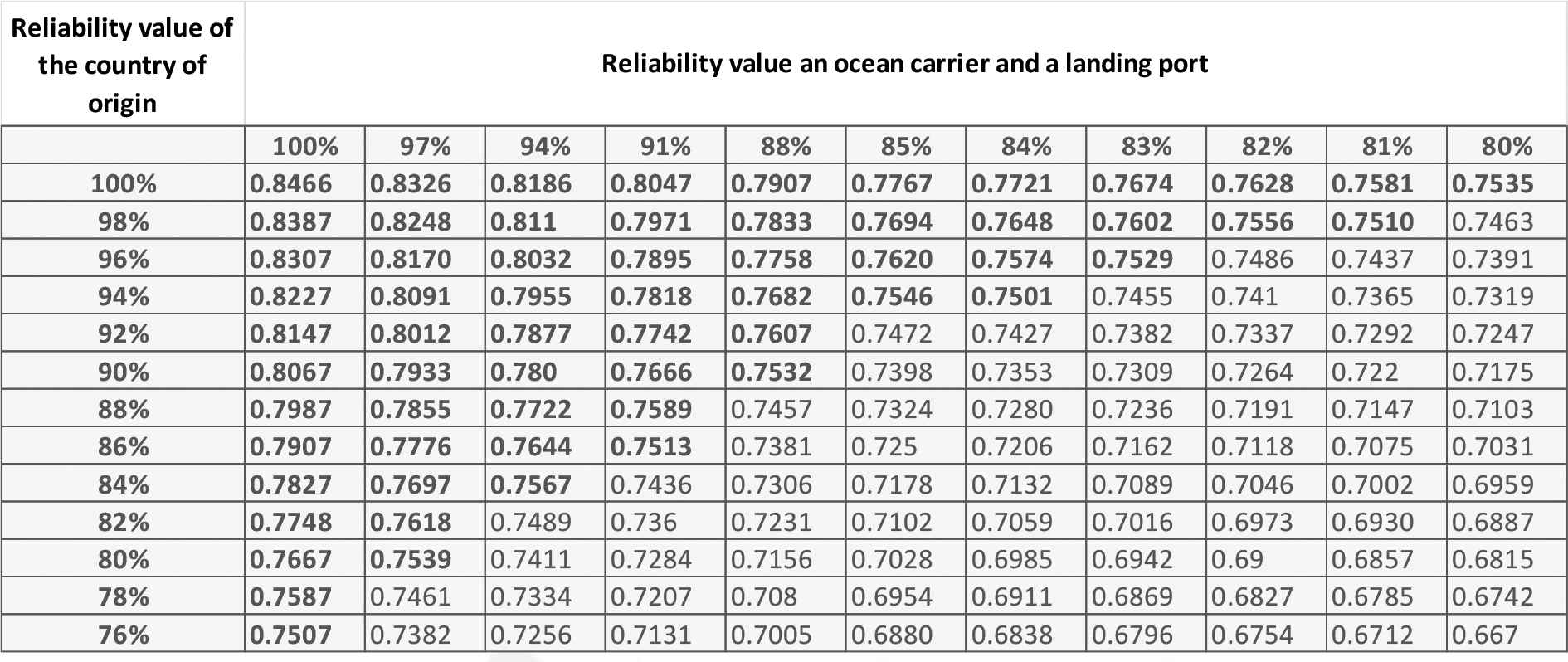
The reliability percentages for the country of origin of the containers (
The limits are defined according to Table 4 [14] so that that every
Histogram for RT and RCO.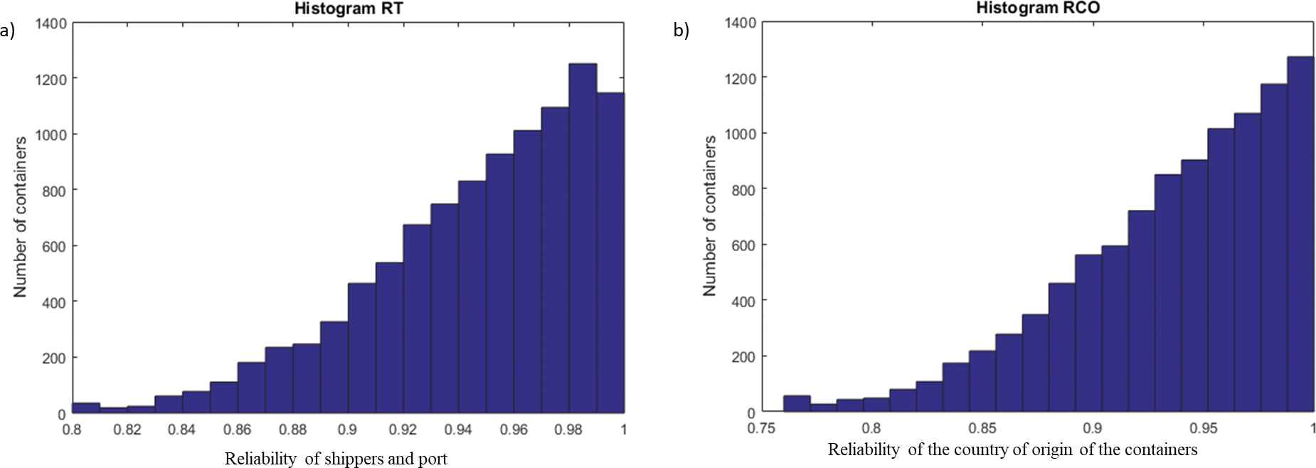
The container
Histogram of the container security scores, SI.
In our case study, the RFID variable represents the reading obtained from the electronic seals on the containers. The ancillary variable,
Then, the ancillary variable,
Then, the ancillary variable,
The following variables are defined:
Then,
The relationship between the
It can be appreciated that in our research, the smuggling and stolen freight events do not occur at the same time. That is, a container could not have been stolen from and contain illegal goods at the same time.
The illegal and legal goods were obtained by generating two ancillary variables using the MATLAB “rand” function with limits between 0 and 1 to obtain uniformly distributed numbers.
Figure 20 shows all the different types of (legal and illegal) goods. Each index in the graphic represents the type of goods. The legal goods are represented by blue: 1 (liquors), 2 (fuels), 3 (tobacco), 4 (medications), 5 (weapons), 6 (raw material), 7 (textiles), 8 (foods) and 9 (manufactured products). The illegal goods are represented by yellow: 1 (liquors), 2 (fuels), 3 (tobacco), 4 (medications), 5 (weapons) and 11 (illegal drugs). Additionally, Table 10 defines the types of goods considered for our case study.
Distribution of the types of legal goods and illegal goods transported.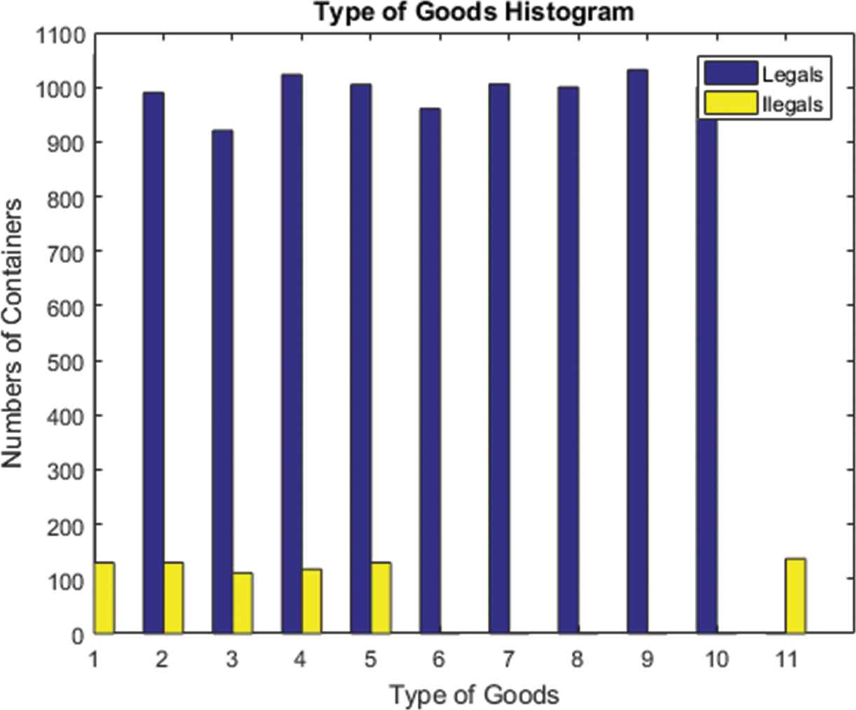
| Goods Transported | Classification of Goods | Classification of Goods According to Type |
|---|---|---|
| 1 liquors | Legal or illegal | Vodka, whiskey, beer, rum, etc. |
| 2 fuels | Legal or illegal | Oil, gasoline, diesel, kerosene, etc. |
| 3 tobacco | Legal or illegal | Cigarettes, cigars, etc. |
| 4 medications | Legal or illegal | Prescription medicines, legal drugs, natural medicines, etc. |
| 5 weapons | Legal or illegal | Firearms, ammunition, bladed weapons, etc. |
| 6 raw material | Legal | Vegetable, animal, mineral, liquid or fossil. |
| 7 textiles | Legal | Different types of cloth, clothes, etc. |
| 8 foods | Legal | Vegetables and animals. |
| 9 manufacturedproducts | Legal | Consumer goods, capital goods and materials and supplies. |
| 11 illegal drugs | Illegal | Cocaine, ecstasy, amphetamines, etc. |
The types of goods used in the case study.
The data generation algorithm assumes that each container only transports one type of goods, and in the case that the container contains illegal goods, it is only one type of illegal goods.
In our case study, we selected X-ray technology as the nonintrusive inspection method among the current existing technological alternatives. X-ray imaging is one of the main nonintrusive technologies for container inspection, and it provides convincing details of the content of large objects such as containers [50], to determine the behaviors of both the X-ray scanner results and the operator. The proposed simulation emulates the behavior of an operator at the moment that an X-ray scan is performed, that is, the operator will see and analyze the data on the container contents, for example, the volume, shape, weight and type of material that it transports. This simulation uses the
The volume factor is given by the following equation:
The shape factor is determined by comparing the shape of the transported goods
The following is the weight factor given by
The material factor is expressed by the following equation:
Two X-ray energy levels were applied (6 MeV and 10 MeV). Using this property, we can classify the contents of a container based on the image provided by the ratio of the different levels of attenuation [42].
CONFLICT OF INTEREST
The authors declare that they have no competing interests.
AUTHORS' CONTRIBUTIONS
The study was conceived and designed by Pablo Cortés and Leonela Morales. Luis Onieva and Ventura Pérez revised the different versions of the research and suggested improvements.The director of the research and final responsible for the revisions was Pablo Cortés. All authors read and approved the manuscript.
ACKNOWLEDGMENTS
The authors wish to acknowledge the financial support of project “Estrategias de diseño microelectronico para IOT en escenarios hostiles” (Ref. TEC2016-80396-C2-2-R) funded by the Programa Estatal de Investigación, Desarrollo e Innovación Orientada a los Retos de la Sociedad for the completion of this work.
REFERENCES
Cite this article
TY  - JOUR
AU  - Leonela Morales
AU  - Luis Onieva
AU  - Ventura Pérez
AU  - Pablo Cortés
PY  - 2020
DA  - 2020/05/21
TI  - Using Fuzzy Logic Algorithms and Growing Hierarchical Self-Organizing Maps to Define Efficient Security Inspection Strategies in a Container Terminal
JO  - International Journal of Computational Intelligence Systems
SP  - 604
EP  - 623
VL  - 13
IS  - 1
SN  - 1875-6883
UR  - https://doi.org/10.2991/ijcis.d.200430.001
DO  - 10.2991/ijcis.d.200430.001
ID  - Morales2020
ER  -