
Sustainable Supplier Selection Based on Regret Theory and QUALIFLEX Method
- DOI
- 10.2991/ijcis.d.200730.001How to use a DOI?
- Keywords
- Sustainable supplier selection; Bounded rantionality; 2-dimension at uncertain linguistic variable; Regret theory; QUALIFLEX
- Abstract
Sustainable supplier selection is the essential core of sustainable supply chain management, which can directly influence the manufacturer's performance and can enormously enhance the manufacturer's competitiveness in the international market. However, most of the previous studies concerning sustainable supplier selection have less focused on the reliability of the decision-makers judgments and the application of regret theory. To fill this gap, we presented an integrated sustainable supplier selection model based on regret theory and QUALItative FLEXible multiple criteria method (QUALIFLEX) under a 2-dimensional uncertain linguistic variable (2-DULV) environment. In the proposed model, 2-DULV including the reliability of evaluation information is employed to handle the uncertainty and vagueness of decision-makers judgments. A similarity-based method is used to derive the decision-makers' weight, and a maximizing deviation model is established to calculate the weights of evaluation criteria. Then an improved QUALIFLEX method based on regret theory is presented to obtain the ranking order of sustainable suppliers. The proposed approach integrates both the superiority of 2-DULV in effectively handling the uncertainty, vagueness, and reliability of evaluation information and the merit of regret theory in dealing with decision-maker's bounded rationality. Finally, a numerical example concerning an automobile manufacturer is provided to validate the effectiveness and feasibility of the presented model.
- Copyright
- © 2020 The Authors. Published by Atlantis Press B.V.
- Open Access
- This is an open access article distributed under the CC BY-NC 4.0 license (http://creativecommons.org/licenses/by-nc/4.0/).
1. INTRODUCTION
In modern society, governments, businesses, and individuals increasingly focus on social responsibility and environmental protection. Sustainable supply chain management (SSCM) can not only reduce environmental pollution in supply chain activities but also enhance the competitive superiority of enterprises, so SSCM is recognized as a new management model, and has attracted more and more attention from researchers and practitioners [1–5]. In the SSCM activities, sustainable supplier selection can be thought of as a conventional supplier selection taking into account the economic, environmental, and social dimensions [6,7]. Sustainable supplier selection plays an important role in the SSCM [8], which both enhances the satisfaction degree and product quality and directly influences the enterprise's environmental performance and competitive advantages. Therefore, how to choose the most suitable sustainable supplier, which is the main focus of this study, has a greatly critical role for enterprises success.
Generally speaking, sustainable supplier selection involves multiple criteria and alternatives, so it's usually called a multi-criteria decision-making (MCDM) problem, including the evaluation and ranking of sustainable suppliers. In the assessment of sustainable suppliers, it's very difficult for decision-makers to represent the evaluation information by a precise number, owing to the complexity of the assessment object and the vagueness and uncertainty of human judgments [9,10]. To handle this problem, many of fuzzy set theories have been used to deal with ambiguity and uncertainty of decision-makers' evaluation, such as interval-valued fuzzy set [11,12], intuitionistic fuzzy set [4,13,14], and uncertain linguistic variable [15]. Although these approaches can effectively deal with vagueness and uncertainty information, it has not addressed the reliability of evaluation information.
In practice, decision-makers not only provide the assessment information on the evaluation object but also express the reliability of their assessment information [16]. To cope with this issue, Liu [16] presented the 2-dimensional uncertain linguistic variable (2-DUVL) concept, including the evaluation information and its reliability, to characterize the ambiguity and uncertainty of decision-makers' assessment information. 2-DULV has been used for various fields under uncertain environment owing to its apparent advantage. For instance, failure mode and effect analysis [17], site selection of power plant [18], and emergency management [19]. Therefore, 2-DULV is utilized to represent the evaluation information of decision-makers in this paper.
After obtaining the evaluation information, several MCDM methods, such as techniques for order preferences by similarity to ideal solution (TOPSIS) [20], preference ranking organization method for enrichment evaluation (PROMETHEE) [21], and weighted aggregated sum product assessment (WASPAS) [22] approaches, were generally used to derive the ranking of sustainable suppliers. Compared with other MCDM approaches, the obvious advantages of the QUALIFLEX approach can be summarized as [23]: (1) Its calculation process is very simple and easy to be operated and implemented; (2) It can effectively deal with cardinal and ordinal information under different criteria in the MCDM problem; and (3) It is especially suitable to handle MCDM problems involving a number of criteria and fewer alternatives. Due to the above merits, Wang et al. [23] developed an integrated MCDM model combining the cloud model and QUALIFLEX method to evaluate the green performance of companies, and Liang and Chong [24] established a hybrid group decision model based on the QUALIFLEX approach to handle the green supplier selection under a complex situation. However, most of the previous studies generally assume that decision-makers are completely rational.
In practical decision activities, decision-maker's behavior is bounded rationality due to their cognition and knowledge limitation, time pressure as well as incomplete information [25]. In this situation, a decision deviation is usually generated between the practical and expected decision results. To handle this situation, prospect theory [26], cumulative prospect theory [27], and TODIM approaches [5] have been used to deal with the sustainable supplier selection problem. Regret theory presented by Loomes and Sugden [28] and Bell [29] is also a bounded rationality theory. It has been extensively applied in different fields, such as risk assessment [30], electronic commerce [31], and development program selection [32] because it well explains and predicts decision-makers' psychological behavior and is simpler than the prospect theory. In addition, according to the advantages of the QUALIFLEX method, QUALIFLEX is suitable to derive the ranking of sustainable suppliers including multiple criteria and limited alternatives. A small number of previous researchers have explored the issue of sustainable supplier selection under bounded rationality context, but there is no study combining regret theory and QUALIFLEX method, especially under the 2-DULV environment. Consequently, it is necessary to propose a hybrid model integrating regret theory and QUALIFLEX approach to fill gaps in existing researches.
To further handle the sustainable supplier selection problem with considering the reliability of evaluation information and decision-makers' psychological behavior, we present a hybrid MCDM model by integrating the regret theory and QUALIFLEX method for evaluating and selecting sustainable suppliers within the 2-DULV environment. Besides, the weights of decision-makers and the weights of evaluation criteria are calculated by an objective weight method. The main contribution of this study to literature can be summarized as follows:
To effectively handle the uncertainty and vagueness of the decision-makers judgments and depict the assessment reliability of decision-makers simultaneously, 2-DULV is utilized to represent the evaluation information of decision-makers.
Decision-makers should be assigned a reasonable weight because of their different experience and knowledge background. In much previous literature, the weights of decision-makers are subjectively given according to their experience. To assign weight reasonably, the weights of decision-makers in this study are obtained by similarity-based methods.
Decision-makers are generally bounded rationality due to the limitations of their cognition and knowledge. To depict this feature, in this paper, an improved QUALIFLEX method based on regret theory (QUALIFLEX-RT) is presented to derive the ranking of sustainable suppliers.
The remainder of this paper is arranged as follows: Related research is provided in Section 2. In Section 3, we propose a hybrid MCDM method utilizing 2-DULVs, regret theory, and QUALIFLEX approach for sustainable supplier selection. A numerical example concerning an automobile manufacturer is provided to implement the proposed approach in Section 4. Finally, Section 5 provides the conclusions of this paper and points out the direction of future studies.
2. RELATED WORKS
In this section, we should introduce the related works, including the methods of sustainable supplier selection, 2-dimensional uncertainty linguistic variable, QUALIFLEX method, and regret theory.
2.1. Methods of Sustainable Supplier Selection
To enhance the competitive advantages, many approaches were employed by enterprises to derive the prioritization of sustainable suppliers in the past decade. According to whether considering the decision-makers' psychological behavior, these methods can be divided into two categories, namely, approaches of complete rationality and methods of bounded rationality. For the former approaches, for example, Li et al. [20] proposed an extended TOPSIS approach to choose a sustainable supplier, using cloud model theory and rough set theory to handle intrapersonal uncertainty and interpersonal uncertainty, respectively. Through combining the revised Simos procedure, PROMETHEE approach, compromise ranking, and robustness analysis, Govindan et al. [21] presented a hybrid model to choose the best green supplier in the food supply chain. Mishra et al. [22] utilized a hesitant fuzzy set to deal with the uncertainty in the green supplier selection and developed an integrated approach based on the WASPAS method. Lu et al. [33] explored the sustainable supplier selection of solar air-conditioner manufacturers by integrating rough set theory and ELECTRE approach. To handle green supplier selection, Wu et al. [34] established a hybrid model based on the best-worst method and vise kriterijumska optimizacija i kompromisno resenje (VIKOR) method. For the latter methods, for instance, Phochanickorn and Tan [26] presented an integrated MCDM model combing fuzzy decision-making trial and evaluation laboratory, fuzzy analytic network process, and prospect theory, for green supplier selection. Liao et al. [27] applied the knowledge of thermodynamics, cumulative prospect theory, and PROMETHEE II method to design an integrating approach for green logistic provider selection. To choose the best green supplier within the environment of interval type-2 fuzzy sets, Qin et al. [5] proposed an extended TODIM approach, which can depict the bounded rationality behavior of decision-makers.
2.2. 2-dimensional Uncertainty Linguistic Variable
The 2-DULV, including the evaluation information and its reliability, was put forward by Liu [16] to characterize the ambiguity and uncertainty of decision-makers' assessment information. 2-DULV adopts I class uncertain linguistic variable
2.3. QUALIFLEX Method
QUALIFLEX approach was initially proposed by Paelinck [36], which is a useful outranking approach in MCDM. QUALIFLEX method is very suitable for solving MCDM problems involving a number of criteria and fewer alternatives [23], so it has been widely employed to deal with various MCDM problems in practice. For example, Chen et al. [37] introduced an extended QUALIFLEX method for dealing with the medical decision-making problem under the interval type-2 fuzzy sets environment. Dong et al. [38] developed a novel QUALIFLEX method based on a cosine similarity to evaluate financial performance. To solve an MCDM issue considering the decision-makers' psychological behavior, Tian et al. [39] presented a decision model by combining the regret theory and QUALIFLEX method to assess the risk of high-tech project investment. Wang et al. [40] proposed a hybrid MCDM approach to handle building energy efficiency retrofitting project selection problem, adopting a picture fuzzy TOPSIS-based QUALIFLEX approach to determine the ranking order of alternatives.
2.4. Regret Theory
Loomes and Sugden [28] and Bell [29] separately proposed the regret theory to characterize the psychological behavior of decision-makers under uncertainty environment. In decision-making, they deem that decision-makers not only take the outcomes of the selected alternative into account but also focus on the results of the chose alternative relative to other alternatives. Regret theory has been extensively applied in different fields, such as risk assessment [30], electronic commerce [31], and development program selection [32] because it well explains and predicts decision-makers' psychological behavior and is simpler than prospect theory.
In regret theory, expected utility function proposed by Von Neumann and Morgenstern [41] is expanded to the perceived utility function, which is consist of the utility function of current selection results and regret-rejoicing function. Assume that
Regret theory was initially used to choose of pairwise alternative. In practice, decision-makers usually face multiple alternatives when they choose the optimal alternative. To deal with this situation, regret theory was extended to general choice sets by Quiggin [44]. Regret theory involving multiple alternatives can be depicted as follows. Let
To our knowledge, existing literature rarely uses the regret theory to handle the problem of sustainable supplier selection considering the bounded rationality of decision-makers, especially in the 2-DULV context. Aiming at filling this research gap, this paper proposes a novel approach combing regret theory and QUALIFLEX method under the 2-DULV environment.
3. PRESENTED MODEL
In this section, we will present an improved QUALIFLEX-RT for sustainable suppliers selection considering the regret aversion behavior of decision-makers under the 2-DULV environment. The flowchart of the presented model is shown in Figure 1.
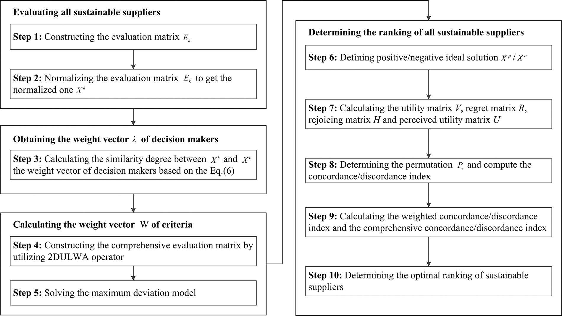
Flowchart of the presented model.
To convenient for description of the proposed approach, the relevant variables applied in this study are provided as follows:
Based on the above variables, the presented QUALIFLEX-RT method for sustainable suppliers selection can be depicted as follows.
3.1. Derive the Weights of Decision-Makers
The similarity-based method is an objective weight method, which can fully utilize the evaluation information provided by decision-makers to derive their weight. Its primary thinking is that the larger the similarity between the decision-maker's evaluation matrix and ideal group evaluation matrix, the greater weight should be assigned to the decision-maker, contrariwise, a smaller weight is assigned. Therefore, to calculate the weights of decision-makers according to a similarity-based method, we firstly define the similarity degree between any two 2-DULVs.
Definition 1.
Let
The ideal group decision matrix can be constructed by 2-dimensional uncertain linguistic weighted averaging operator (2-DULWA) [35].
If the evaluation matrix
After that, the comprehensive evaluation matrix
3.2. Calculate the Weights of Criteria
Generally speaking, if the values
According to the thinking of maximizing deviation method, the maximizing deviation model can be constructed as follows:
To solve the equation above, Lagrange multiplier function is constructed as follows:
Let the first-order partial derivative of Eq. (7) be 0,
Then we have
Normalize the criteria weight, we have
3.3. Rank the Sustainable Suppliers by QUALIFLEX Method Based on Regret Theory
According to the evaluation matrix and the weights of decision-makers and criteria, we presented an improved QUALIFLEX approach based on regret theory to determine the ranking of sustainable suppliers.
Define the positive ideal solution (PIS)
Then, depending on the utility function, the utility matrix of sustainable suppliers is calculated by
According to the regret-rejoicing function, the regret and rejoicing matrices of sustainable suppliers can be constructed as follows:
After that, the perceived utility matrix
For the
In the
Considering the weight vector
For the permutation
According to the Eq. (20), we can know that the higher the comprehensive CDI value
Based on the analysis above, the selection flow of sustainable supplier under 2-DULV environment can be summarized as follows:
Step 1: Obtain the evaluation information of supplier
Step 2: Normalize the evaluation matrix
For the criterion
Step 3: Determine the weight vector
Step 4: Construct the comprehensive evaluation matrix
Step 5: Establish and solve the maximum deviation model (Eq. (6)) to derive the weight vector
Step 6: Define thePIS
Step 7: Calculate the utility matrix
Step 8: Determine the permutation
Step 9: Calculate the weighted concordance/discordance index (WCDI)
Step 10: Determine the optimal ranking order of sustainable suppliers by choosing the permutation with the greatest comprehensive CDI
4. NUMERICAL EXAMPLE
In this section, a case of an automobile manufacturer in China is provided to verify the effectiveness and applicability of the presented method. Since entering the car field in 1996, the automobile manufacturer has achieved rapid development because of flexible operating mechanisms and continuous independent innovation. Therefore, it was named the first batch of national innovative enterprises. Moreover, for four consecutive years, it has entered the top 10 of China's automobile industry. However, the automobile manufacturer is drastically undertaking environmental protection pressure since the implementation of the new Environmental Protection Laws of the People's Republic of China on January 1, 2015. To cut down the environmental protection pressure and improve the competitive advantage simultaneously, the automobile manufacturer has to reevaluate the performance of suppliers from the economic, environmental, and social aspects. To this end, the proposed method in this paper is used for helping the automobile manufacturer to select the best supplier for purchasing the relative components of new automobile product. Ten evaluation criteria relevant to sustainable supplier selection, which collected from previous literatures [5,7], are identified as the total product life cycle cost (
4.1. Implementation of the Presented Model
In this subsection, the calculation procedure of the presented approach is described as follows:
Step 1: The evaluation matrices
| Criterion | ||||
|---|---|---|---|---|
DULV, 2-dimensional uncertain linguistic variable.
2-DULV evaluation matrix
| Criterion | ||||
|---|---|---|---|---|
DULV, 2-dimensional uncertain linguistic variable.
2-DULV evaluation matrix
| Criterion | ||||
|---|---|---|---|---|
DULV, 2-dimensional uncertain linguistic variable.
2-DULV evaluation matrix
| Criterion | ||||
|---|---|---|---|---|
DULV, 2-dimensional uncertain linguistic variable.
2-DULV evaluation matrix
Step 2: Due to the criteria
Step 3: The similarity degree is calculated by using Eq. (3), then weight vector of decision-makers can be obtained
Step 4: The comprehensive evaluation matrix
| Criterion | ||||
|---|---|---|---|---|
The comprehensive evaluation matrix
Step 5: Depending on Eqs. (8–12), we can calculate the weight vector
Step 6: The PIS
| Criterion | PIS | Criterion | NIS |
|---|---|---|---|
PIS, positive ideal solution; NIS, negative ideal solution.
The positive/negative ideal solution
Step 7: Utilizing Eqs. (13–16), we can obtain the utility matrix
Step 8: Define the permutation
| Permutation | Permutation | Permutation | Permutation | ||||
|---|---|---|---|---|---|---|---|
Permutation of all sustainable suppliers.
Then the CDI
| |
|
|
|
|
|
|||||
| |
|
|||||||||
| |
|
|
|
|
|
|||||
| |
|
|
||||||||
| |
|
|
|
|
|
|
||||
| |
|
|
|
|
|
|
|
|
CDI, concordance/discordance index.
The results of CDI for permutation
Step 9: According to Eq. (19), the WCDIs for all permutations are listed in Table 9. Then, using the Eq. (20), the CCDI for all permutations are shown in Table 10.
| WCDI | WCDI | WCDI | WCDI | ||||
|---|---|---|---|---|---|---|---|
| |
|
|
|
||||
| |
|
||||||
| |
|
|
|
||||
| |
|
|
|||||
| WCDI | WCDI | WCDI | WCDI | ||||
| |
|
||||||
| |
|
|
|
||||
| |
|||||||
| |
|
||||||
| |
|||||||
| WCDI | WCDI | WCDI | WCDI | ||||
| |
|
|
|||||
| |
|
||||||
| |
|
||||||
| |
|
|
|
||||
| |
|
||||||
| |
|||||||
| WCDI | WCDI | WCDI | WCDI | ||||
| |
|
||||||
| |
|
|
|
||||
| |
|
|
|
||||
| |
|
|
|
||||
| |
|
|
|
||||
| |
|
||||||
| WCDI | WCDI | WCDI | WCDI | ||||
| |
|||||||
| |
|
||||||
| |
|
|
|||||
| |
|
||||||
| WCDI | WCDI | WCDI | WCDI | ||||
| |
|
||||||
| |
|
|
|||||
| |
|
|
|||||
WCDI, weighted concordance/discordance index.
The results of WCDI for all permutations.
| CCDI | CCDI | CCDI | CCDI | CCDI | CCDI | ||||||
|---|---|---|---|---|---|---|---|---|---|---|---|
| |
|
|
|||||||||
| |
|
|
|||||||||
| |
|
|
|||||||||
| |
|
|
CCDI, comprehensive concordance/discordance index.
The results of CCDI for all permutations.
Step 10: The optimal permutation can be obtained by descending order of CCDI value, that is, permutation
4.2. Sensitivity Analysis
To illustrate the influence of different risk aversion coefficient
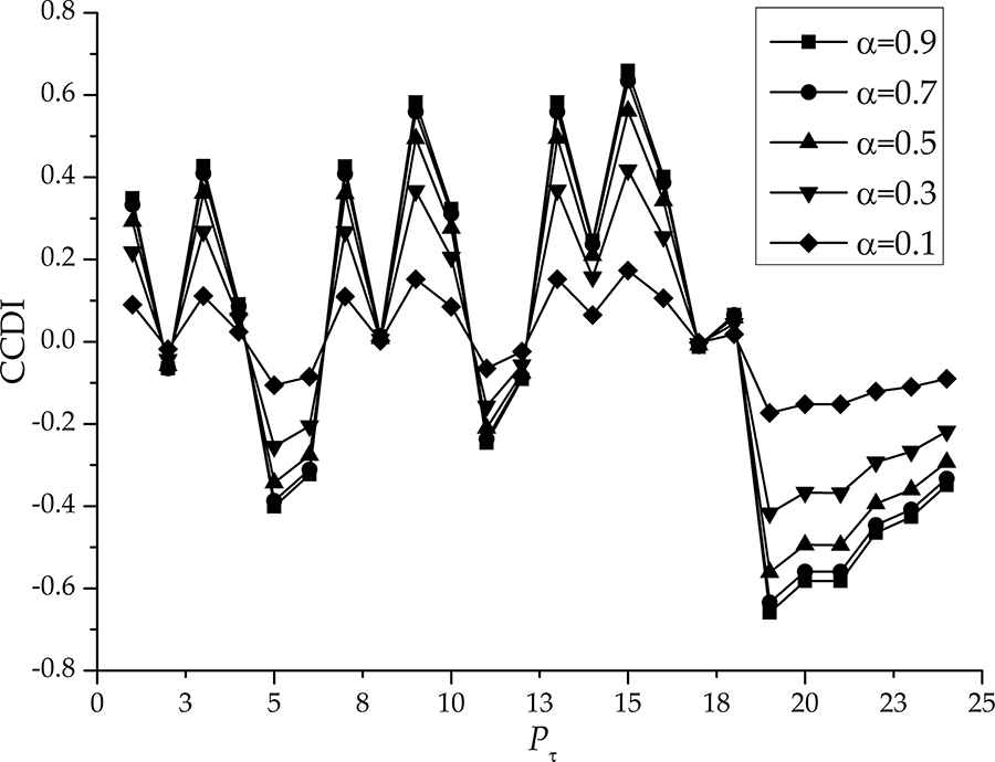
The CCDI values with different
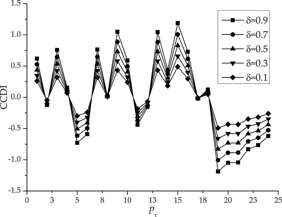
The CCDI values with different
From Figure 2, we can know that the CCDI values of all permutations have changed with different
4.3. Comparisons and Discussion
To validate the effectiveness and advantage of the presented method (QUALIFLEX-RT), some existing approaches are used to conduct a comparative analysis, including the TODIM approach [5] and the WASPAS method [47]. Besides, we also adopted the approach based on the 2-DULWA operator to derive the priority of sustainable suppliers. Utilizing the QUALIFLEX-RT approach and the three methods mentioned above, the ranking results of four sustainable suppliers are displayed in Figure 4.
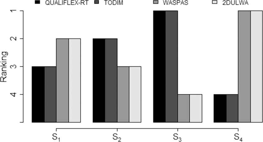
The ranking results of different methods.
As shown in Figure 4, we can observe that the ranking result of sustainable suppliers determined by the WASPAS method is the same as that derived by the 2-DULWA operator, that is,
The main reason that results in the ranking difference is that the WASPAS method integrating the weighted sum model and the weighted product model and the approach based on the 2-DULWA operator assume that the decision-makers are completely rationality. This assumption is unreasonable in the decision-making process. Therefore, the result obtained by the QUALIFLEX-RT approach introducing the regret theory is more reasonable because it takes into account the regret aversion behavior of decision-makers. Another reason may be that the presented approach uses the 2-DULV including the reliability of evaluation information to evaluate the sustainable suppliers. Whereas the WASPAS method adopts interval type-2 fuzzy sets to evaluate the performance of sustainable suppliers, which may lead to a biased result due to not incorporate the reliability of the evaluation information.
The main reason behind the consistent ranking between the TODIM method and the QUALIFLEX-RT approach can be explained that the bounded rationality behavior of decision-makers is considered by the two methods. The same ranking results also validate the effectiveness and feasibility of the presented approach. Consequently, the ranking result of sustainable suppliers determined by the QUALIFLEX-RT is accurate and reasonable.
Compared with the 2-DULWA operator, the TODIM method and the WASPAS approach, the QUALIFLEX-RT method offers the following advantages: (1) The presented approach adopts the 2-DULV to assessment the performance of sustainable suppliers, which can better describe the ambiguity, uncertainty, and reliability of decision-makers judgment; (2) The QUALIFLEX-RT method based on the regret theory is utilized to determine the ranking of sustainable suppliers, which can better depict the decision-makers' bounded rationality behavior in the decision-making process.
Although the presented model has some advantages, there are also existing several drawbacks, which need to be further explored in the future. Firstly, the proposed method does not consider the interdependent relationship between the evaluation criteria, but these interactions generally exist in the sustainable supplier selection. In the future, we can introduce the Choquet integral [48] and power aggregation operator [49] into the proposed model to depict this interdependent relationship. Secondly, the consensus level between decision-makers is an important factor in decision-making which has been studied by some researchers [50,51], therefore we can include the consensus level in future sustainable supplier selection study. Furthermore, the presented method in this paper can be utilize to handle other MCDM problems, such as emergency management [52], site selection [53], and risk assessment [54], and so on, to further illustrate its effectiveness.
4.4. Managerial Implications
The main intent of this study helps managers of companies to select the best sustainable supplier for enhancing competitive advantage by developing a hybrid model combing 2-dimensional uncertain linguistic variable, regret theory, and QUALIFLEX method. Consequently, managerial implications are as follows:
The presented model by adopting 2-DULV to express the assessment information offers an effective and flexible approach for enterprise managers to cope with a multitude of vagueness and uncertainty information of decision-makers' evaluation in the sustainable supplier selection.
The presented model adopted regret theory to depict the psychological behaviors of decision-makers under the uncertain environment. In previous studies, the behavior experiment results indicate that decision-makers' psychological behaviors have significant influences on the ranking results of alternatives. Consequently, enterprises' managers should consider the psychological behaviors of decision-makers in sustainable supplier selection.
Through conducting the proposed method, the enterprise can enhance the performance and competitiveness of its supply chain by selecting the best sustainable supplier, and suppliers can discover their manage shortcomings and propose some corrective actions. To do so, between enterprises and their suppliers can establish a strategical partner relationship.
5. CONCLUSION
This paper investigates the sustainable supplier selection problem by presenting a novel model integrating the regret theory and the QUALIFLEX approach under a 2-DULVs environment. In this model, 2-DULVs are employed by decision-makers to evaluate the performance of sustainable suppliers on criteria. A similarity degree method is utilized to determine the weight of decision-makers. Then we established a maximizing deviation model to calculate the criteria weights, and an improved QUALIFLEX approach based on the regret theory is used for deriving the ranking result of sustainable suppliers. Ultimately, a numerical example of an automobile manufacturer is provided to demonstrate the effectiveness and feasibility of the presented model. Moreover, the results of a comparative analysis show that the presented method is the ability to describe the bounded rationality behavior of decision-makers and is an effective approach to determine the ranking order of sustainable suppliers.
CONFLICT OF INTEREST
The authors declare they have no conflicts of interest.
AUTHORS' CONTRIBUTIONS
Concept of this study, Limei Liu, Zhongli Bin, and Biao Shi; methodology, Limei Liu and Wenzhi Cao; writing-original draft preparation, Limei Liu; writing-review and editing, Zhongli Bin and Biao Shi.
ACKNOWLEDGMENTS
This research was funded by the National Social Science Fund of P.R. China (Grant No.18BGL181).
REFERENCES
Cite this article
TY  - JOUR
AU  - Limei Liu
AU  - Zhongli Bin
AU  - Biao Shi
AU  - Wenzhi Cao
PY  - 2020
DA  - 2020/08/10
TI  - Sustainable Supplier Selection Based on Regret Theory and QUALIFLEX Method
JO  - International Journal of Computational Intelligence Systems
SP  - 1120
EP  - 1133
VL  - 13
IS  - 1
SN  - 1875-6883
UR  - https://doi.org/10.2991/ijcis.d.200730.001
DO  - 10.2991/ijcis.d.200730.001
ID  - Liu2020
ER  -