
Discovering Potential Partners via Projection-Based Link Prediction in the Supply Chain Network
 , Qian Chen
- DOI
- 10.2991/ijcis.d.200813.001How to use a DOI?
- Keywords
- Supply chain network; Resilience; Potential partners; Link prediction
- Abstract
As reserving a certain number of potential partners plays a significant role in alleviating existing partners' collaborative interruption risks, we investigate the process of discovering potential partners to improve the supply chain network's resilience. Most of the existing research confines its focus on discovering potential partners in the supply chain on the basic of sufficient partners' information, but very few works consider discovering potential partners in the supply chain network according to the structure of the supply chain network when the partner information is insufficient. In this situation, a novel model which applies projection-based link prediction method to discover potential partners in the supply chain network is proposed. The proposed model is composed of three stages. The first stage is predicting the candidate partnerships links based on the projection one-model graph which is transformed from the supply chain network according to its structure. The second stage is discovering potential partners by comparing the acquired connectivity of candidate partnership links with the maximal connectivity of existent partnerships. In the third stage, a resilience evaluation framework considering the both connectivity and flexibility indexes is presented to determine whether the supply chain network's agility is improved. In the experimental design, a supply chain network which is formed from a real dataset containing mobile phone suppliers, manufacturers and packers is used to evaluate the proposed algorithm's prediction accuracy. The results reveal that the algorithm achieves highest area under curve (AUC) scores and the supply chain network's resilience is improved by discovering potential partners.
- Copyright
- © 2020 The Authors. Published by Atlantis Press B.V.
- Open Access
- This is an open access article distributed under the CC BY-NC 4.0 license (http://creativecommons.org/licenses/by-nc/4.0/).
1. INTRODUCTION
Traditionally, discovering potential partners in the supply chain is considered as a process of ranking candidates according to sufficient partners' information, such as the factors of cost, quality, delivery time, supply capacity and the precedence of tasks, etc. However, in order to adapt to the course of economy and technology globalization [1], discovering potential partners in the supply chain has evolved into discovering partners in the supply chain network. Compared with the simple linear supply chain, the structure of supply chain network is complex. As a result, there is now a widespread need to take into consideration the influence of the supply chain network structure on discovering potential partners [2,3]. To characterize the supply chain network's structure, some models on the basic of network theory have been presented [4], in which the network involves a series of nodes and links which refer to the suppliers, manufactures, packers and connections among them respectively. In order to make transactions or provide products and services, companies in the supply chain network work on interplay relationships with other enterprises, which generates various links including cooperation links, material links, information links, capital links and logistics links [5].
Recently, discovering potential partners in the supply chain network has led to a spectrum of attention by researchers. As stated by Hua, Sun and Xu [5], discovering potential partners in the supply chain network plays a significant role when enterprises are facing the interruptions of cooperations with their existing partners. Mensah et al. [6] put emphasis on the necessity of discovering potential partners by revealing that any suppliers' unexpected events may have a catastrophic influence on operations of the supply chain and cascade throughout the entire supply chain network. To understand how to discover potential partners in the supply chain network, others have suggested adopting the mathematical approach to explore this process. Salo and Jarimo [7] established a mixed-integer linear model to discover candidates in the virtual enterprise supply chain network. Sarkis et al. [8] proposed a strategic discovering agile candidates model on the basic of analytical network process (ANP) methodology. Guneri and Yucel [9] provided a weighted additive fuzzy programming method for predicting potential partners in the supply chain network. Chuang and Yeh [10] introduced two multi-objective genetic algorithms building an optimum mathematical discovering potential partners model. Han and Shin [11] applied fuzzy sets theory (FST) to discovering potential partners in the supply chain network.
Although the above methods have advantages in different contexts, partner information's scarcity is a large obstacle of exploring the potential partnerships in their implementations. Some papers aiming at discovering potential partners have tried to employ FST to overcome the incompleteness and uncertainty of partner information in the supply chain network [11–14]. The FST is an effective method to handle uncertain information, which can deal with the incomplete and uncertain information about the candidates and their performances [12]. Zhao et al. further pointed out that the FST can be applied to solve the problem of prediction [15]. However, the method of using fuzzy sets and fuzzy logic theories ignores the structure of the supply chain network and needs to select an adaptive initial set-point to complement an optimum value search. If the structure of the network is complex, the loss ratio and the delay must be increased.
In reality, discovering potential partners in the supply chain network can effectively alleviate the bad influence that existent cooperation partnership disruptions bring. Once the supply chain network members' cooperation is interrupted, the situation of sharp increase in supply costs, loss in profits, even brand damage and worse social impact will appear and the supply chain network will have difficulty in restoring normal operations in a short period of time. The purpose of this paper is to present a model of discovering potential partners to reconstruct possible supply chain network on the basic of projection-based link prediction in the supply chain network to avoid the losses in the early stage. The innovation of the work lies in that we shed light on how to use projection-based link prediction to discover potential partners in the supply chain network. This application of link prediction provides a technical basic for the further supply chain management's advance. Specifically, the contributions of this article are the following:
The model depicting discovering potential partners in the supply chain network as predicting potential partnerships links in the network composed of participating enterprises nodes is proposed.
Projection-based link prediction converts the supply chain network into projection one-model graphs according to the supply chain network's structure and compares the acquired connectivity of candidate partnership links with the maximal connectivity of existent partnerships to discover potential partners.
The resilience evaluation framework of supply chain network considering the connectivity and flexibility index is presented to evaluate the supply chain network agility after discovering potential partners.
The reminder of this article is arranged as follows: Section 2 introduces the concepts and applications of link prediction. Section 3 depicts the link prediction for discovering potential partners in the supply chain network. Section 4 proposes a novel model based on projection-based link prediction. Section 5 presents the experiments and results of proposed algorithm in a real mobile phone supply chain network. Section 6 makes conclusions and provides directions for future research.
2. THEORETICAL BACKGROUND
Discovering potential partners in the supply chain network is able to be implemented successfully by formulating evaluation criteria according to valid partner information, but it will be difficult under the circumstance of partner information inaccuracy. There is a novel way of discovering potential partners in the supply chain network, which uses link prediction to predict potential partnerships links by analyzing the supply chain network's structure. Link prediction refers to how to make use of the structure of network or the label of known nodes to predict the connection probability of potential links which have not been connected yet in the network.
Link prediction has been applied to many significant fields for various goals. In the popular online social networks including Facebook and LinkedIn, a list of people you may know can be suggested [16]. In the ecommerce websites, personal recommendations can be generated to recommend products that customers most likely need [17]. Especially, the bipartite network is a classical form of complex networks in link prediction, where the nodes are divided into two disjoint parts, and the links connect with nodes which belong to different parts [18]. Link prediction in the bipartite network has gained a large-scope applications. For example, in the scientist-papers cooperation network [19], long-term collaboration trends in scientific collaborations are able to be identified by using link prediction. In the author-topic network, appropriate topics can be provided for academic authors according to the citations number of a publication and the condition of collaboration between authors [20]. In the term-document network [21], documents which have possibility to have substantial impact in a term can be discovered. In the club members–activities network [22], the relationships of club members can be predicted which is similar to recommend friends in the social network. In the disease–gene, drug–target and drug–therapy network, interactions in medical sciences also can be predicted [23].
Recently, many scholars have proposed various approaches to predict potential links in bipartite networks [24–29]. Benchettara et al. [24] introduced new indicators of network structure characteristics to measure the appearance possibility of potential links and applied classical supervised machine learning approaches to modelling prediction problems. Kunegis et al. [25] used the odd element of the underlying spectral conversion to transform graph kernels into bipartite networks resulting in several new link predictions. Li and Chen [26] proposed a recommendation approach based on kernel to predict whether there existed a potential link. Shams and Haratizadeh [27] presented a SibRank approach, which represented users' preferences as a signed bipartite network in order to improve the neighbor-based collaborative ranking methods. Zhang et al. [28] identified false and missing links in bipartite networks by employing the processes of local diffusion to evaluate the internal similarity. Chang et al. [29] predicted potential links in Wikipedia which is a characteristic bipartite network by making use of a strengthened supervised machine learning method.
A common way of predicting potential links in a bipartite network is to project the bipartite network into a projection one-model graph. Allai et al. [30] introduced novel approaches of the weighted projection graph and internal links to analyze bipartite networks. In their approaches, all nonexistent links are listed, then those whose internal links weights are greater than predetermined threshold value are potential links. However, listing all nonexistent links spent a large amount of calculation time and the selection of a suitable threshold in advance is difficult. Aslan and Kaya [20] put forward a link prediction approach on the basic of strengthening weighted projection then applied it to discovering the possible citation links in a real-world author-topic network. The drawback of their method lies in that the dataset and application affect the selection of threshold greatly. Gao et al. [31] presented an approach that predicts candidate node pairs by mapping the bipartite network onto a projected graph. Due to lack of a proper threshold value, it is difficult to assess whether potential links are superior to previous links. To fill these gaps, we presented a model on the basic of projection-based link prediction [31] to discover potential partners in the supply chain network.
Mathematically, the concept of link prediction is defined in the following: Suppose
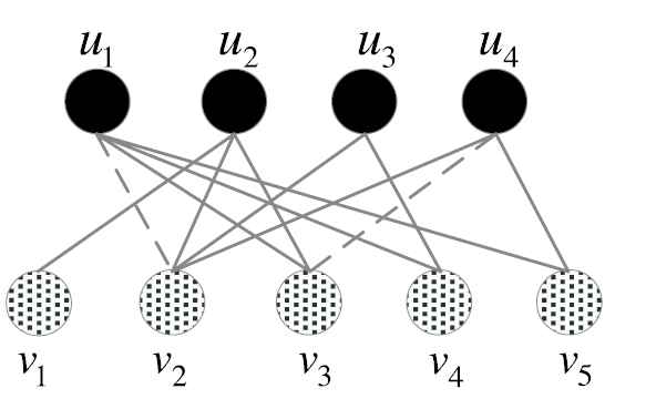
Discovering potential links of the bipartite network.
3. THE LINK PREDICTION FOR DISCOVERING POTENTIAL PARTNERS IN THE SUPPLY CHAIN NETWORK
Figure 2 illustrates a supply chain network consisting of participating enterprises such as suppliers, manufacturers, packers, distributors and retailers, spans undirected links representing partner interrelationships between upstream and downstream parties along the network. Discovering potential partners in the supply chain network is imperative stimulated by the dynamic market. To launch better cooperation, existing enterprises may consider choosing better parties as their potential partners. Although some enterprises may have their relatively fixed partners, they still have the rights to reserve a number of potential partners to avoid economic losses in case of market failure or cooperation disruption. Discovering potential partners in the supply chain network can be viewed as predicting potential partnerships links in a network composed of participating enterprise nodes.
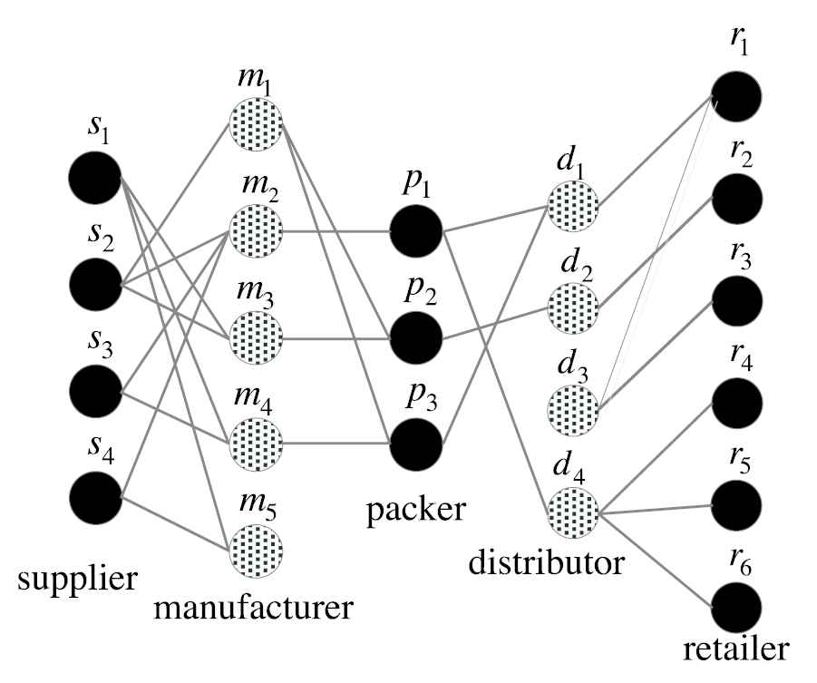
A traditional supply chain network.
The network shown in Figure 2 can be divided into four bipartite networks comprising of suppliers-manufacturers, manufacturers-packers, packers-distributors, distributors-retailers relationship, as displayed in Figure 3. Suppose
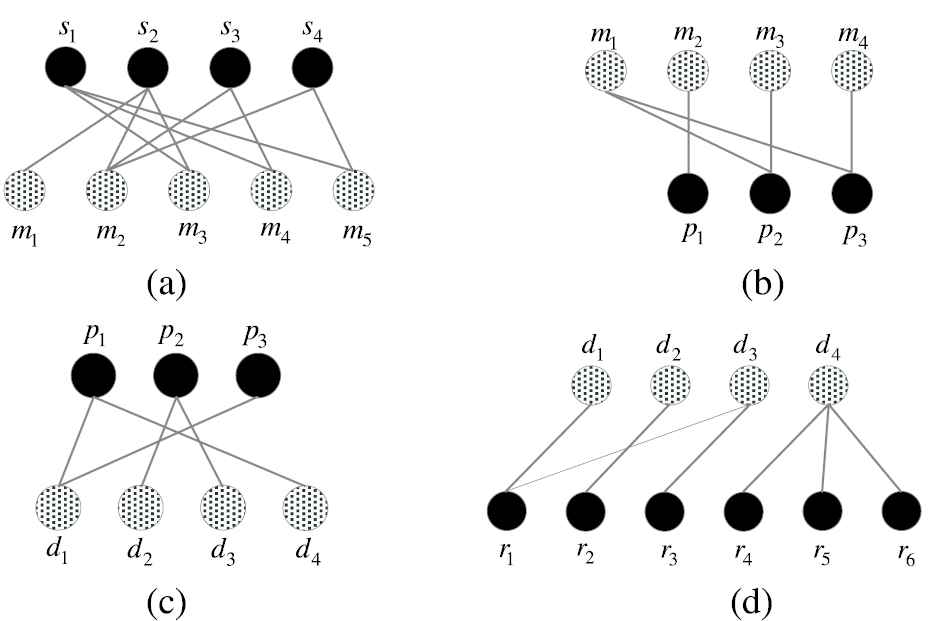
A traditional supply chain network is divided into four bipartite networks: (a) suppliers–manufacturers bipartite network, (b) manufacturers–packers bipartite network, (c) packers–distributors bipartite network, (d) distributors–retailers bipartite network.
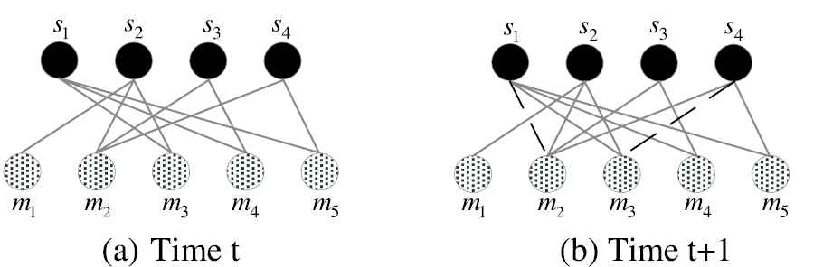
Prediction of potential partnerships links at time in a suppliers–manufacturers bipartite network at time t.
4. THE PROPOSED MODEL
A model of discovering potential partners was proposed to improve the supply chain network's resilience. It is made up of three significant stages. Firstly, the candidate partnerships links are predicted according to the supply chain network's structure and its projection one-model graph. Secondly, comparing the acquired connectivity of candidate partnership links with the maximal connectivity of existent partnerships to discover potential partners. Thirdly, to determine whether the supply chain network's resilience is improved, we presented the resilience evaluation framework according to the supply chain network connectivity and flexibility index.
In the model, to predicate the potential partnerships links in the supply chain network, the suppliers-manufactures bipartite network is first converted into projection one-model graphs, which is given in Definition 1.
Definition 1.
Let
Similarly, its M-projection one-model graph is defined as a unipartite graph
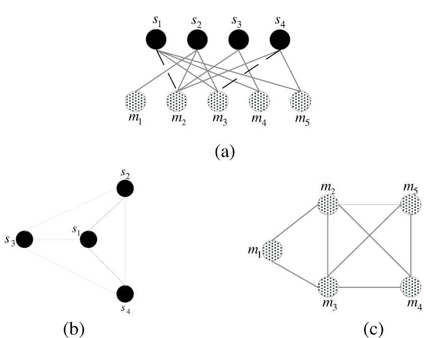
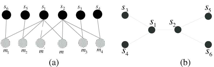
A suppliers–manufacturers bipartite network is projected into two one-model graphs: (a) suppliers–manufacturers bipartite network, (b) S-projection one-model graph, (c) M-projection one-model graph.
4.1. Predicting Candidate Partnership Links
To discover the potential partners in the bipartite network, we define the candidate partnership link based on the projection one-model graph.
Definition 2.
Let
For example, the unlinked node pair
To estimate the connecting possibility of candidate partnership links, pattern and pattern covered by the candidate partnership are given in Definitions 3 and 4 respectively.
Definition 3.
Suppose
Definition 4.
Suppose
where
There are one or more patterns can be covered by a candidate partnership link in the projection one-model graph. If a candidate partnership link covers more patterns, the connecting possibility of the candidate partnership link will be higher. Thus, the number of patterns covered by the candidate partnership link can represent the probability of its link appearance.
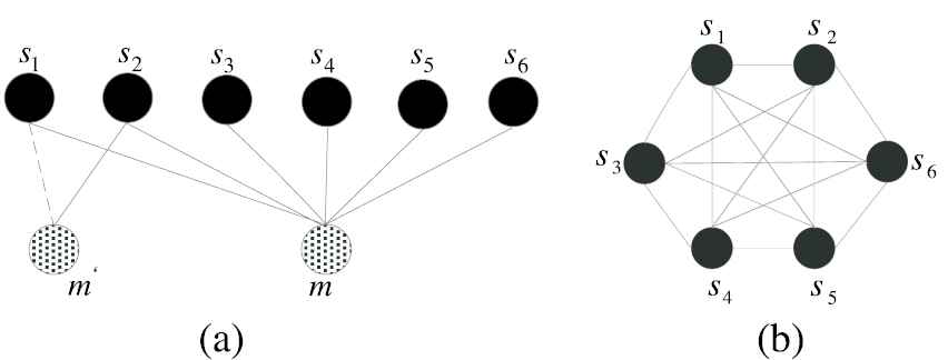
In Figure 5(a), the concrete links
We also note that the number of patterns which are covered by the candidate partnership link
4.2. Discovering Potential Partners
In this work, the potential partners set is extracted by using both the structural information of the weighted projection network and the candidate bipartite network with connectivity values.
In a projection one-model graph, each pattern is given a weight to its corresponding link. To obtain the pattern weight of
The number of communal partners of nodes
The pattern covered by the candidate partnership link is showed by a link in the projection one-model graph. Every link
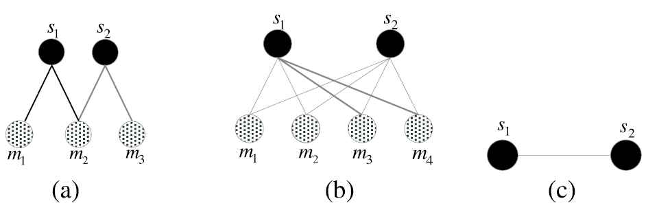
Two different suppliers–manufacturers bipartite networks and their projection one-model graph.
The degree of communal partners of nodes
In the pattern
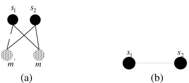
Candidate partnership link and its projection.
Candidate partnership link and its projection.
The degree of nodes
The degree of nodes
Candidate partnership link and its projection.
According to the above analysis, the pattern weight can be defined as follows:
Definition 5.
Suppose that
In Definition 5, if
In the model, each candidate partnership link is given to an indicator named connectivity, which is a metric of the candidate partnership link appearance probability. The connectivity of candidate partnership link can be defined in the following:
Definition 6.
The connectivity of candidate partnership link
In the Definition 6, the connectivity of the candidate partnership link
A significant index of network structure, called clustering coefficient of link, characterizes the connectivity between a link's two corresponding nodes and other surrounding nodes [33]. With the aim of discovering potential partners in the supply chain network accurately, we adopt the link's clustering coefficient to measure the existent partnership link's connectivity.
Definition 7.
The connectivity of existent partnership link
Since the weight of pattern reveals the links' similarity, the connectivity of candidate partnership link indicates the probability of candidate partnership link to be connected. Only when the connectivity of the candidate partnership link is greater than or equal to the maximal connectivity of existent partnership, will we recognize it as a potential partner relationship.
4.3. The Resilience Evaluation Framework
The resilience evaluation framework is a metric of a supply chain network's capability of making preparations for accidents, making response to interruptions and reverting to the same or a better operation state and thus includes network rejuvenation [34]. The framework takes the connectivity and flexibility of the supply chain network as criteria to assess the resilience improvement after discovering potential partners. The connectivity index quantifies connecting changes of the supply chain network after discovering potential partners. The analysis of supply chain network's flexibility can unveil configuration variation of the network which is affected by discovering potential partners [35,36]. Connectivity index indicates the speed of the supply chain network respond to market disruptive events and flexibility index means the capacity of transforming the supply chain network's range number and range heterogeneity to handle a series of turbulent market changes [37]. According to Scholten and Schilder [38], increased connectivity value and flexibility value resulted in a more resilient supply chain network.
The resilience evaluation framework is formulated as follows:
It evaluates the ratio of total connectivity of links after discovering potential partners to the connectivity of the existent network. If the value of connectivity is greater than 1, it means that the connecting relationship of the supply chain network is improved by introducing new potential partners.
The flexibility of the network is depicted as
4.4. The Algorithm of Proposed Model
Based on the proposed model, we present a discovering potential partnerships (DPPs) algorithm in supply chain bipartite network. The first step is to projectively transform the given suppliers–manufacturers bipartite network into projection one-model graphs. The second step is to calculate the weights of patterns covered by the candidate partnership links in the light of formula (1). Then, the connectivity of each candidate partnership link
Algorithm of discovering potential partners
Input: The suppliers-manufactures bipartite network
Output: Potential partners and the resilience comparison results of original and post-experiment supply chain network;
Step 1: Construct the set of patterns
1.
2. For each supplier node
3. For each manufacturer node
4. For each supplier node
5.
6. End for
7. End for
8. End for
Step 2: Compute the weight of each pattern
9. For each link
10. Compute the weight of pattern
11. End for
Step 3: Compute the connectivity of candidate partnership link
12. For each supplier node
13. For each partner
14. For each manufacturer node
15. If
16.
17. End if
18. End for
19. End for
20. End for
Step 4: Compute the connectivity of existent partnership link according to formula (4);
21. If
22. Output potential partners.
23. End if
Step 5: Evaluate the resilience of supply chain network
24. For original and post-experiment supply chain network
25. Compare the
26. Calculate
27. Output the resilience comparison results of original and post-experiment supply chain network.
28. End for
5. ANALYSIS AND DISCUSSION OF THE EXPERIMENTAL RESULTS
To evaluate the proposed DPP algorithm for discovering potential partners in the supply chain network, we test it by performing experiments on a realistic mobile phone bipartite supply chain network. The experiments were carried out on computer with 4GB memory and operating system of Intel Core i5 Windows 7. The algorithm was operated in Matlab R2018a and the experimental results are visualized by Gephi.
5.1. Dataset
A real mobile phone supply chain network dataset is used to perform our experiments. Unlike some of the traditional link prediction literatures which use experimental dataset available to be downloaded from open-source and free websites, such as www.gephi.org, www.linkprediction.org, the dataset in this work is collected and integrated from the Mobile Phone Newspaper, Economic Daily, the Logistic Business of Headscm and Alibaba.com. In our test, we consider cellular phone brands such as Apple, Huawei and Mi and their suppliers, manufactures and packers.
Figure 10 illustrates a bipartite network of mobile phone suppliers and manufacturers. It depicts the participation of 125 suppliers and 9 manufacturers. They are marked as yellow and green respectively in the figure. If a supplier provides the manufacturer some mobile components such as chips, batteries and screens, the corresponding nodes will be connected by a link in the bipartite network. There are 941 links in total connecting suppliers with manufacturers. Figure 11 shows a manufacturers–packers bipartite network. The dataset characterizes 23 firms including 9 manufacturers and 14 packers, as marked in green and red in the graph. Each link reflects a manufacturer cooperates with a packer, and there are totally 126 of it shown in the figure.
Original structure of suppliers–manufacturers bipartite network.
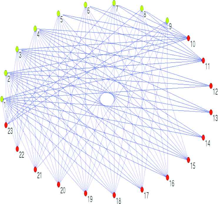
Original structure of manufacturers–packers bipartite network.
5.2. Evaluation Metric
To evaluate the prediction result of the DPP algorithm, we divide all the existent links into
AUC was initially a metric to assess the prediction quality of the algorithms [39], which refers to the area under the receiver operating characteristic (ROC). ROC curve aims to assess the effect of classifier. In our experiments, the AUC value is able to be regarded as the probability when the similarity score of an existent link is higher than the similarity score of a nonexistent link. To compare the links' similarity scores, existent links and nonexistent links can be chosen randomly. In
In general, if the AUC score is higher, the prediction quality of the proposed algorithm is better. It is clear that the highest AUC score in formula (8) is 1, which represents a complete correct result. In fact, if all similarity scores are random, the AUC score is 0.5 approximately.
5.3. Comparison Baselines
With the goal of comparing the proposed algorithm's AUC value with other link prediction algorithms' AUC value, we choose three algorithms from the baselines of Preferential Attachment (PA) index, Local Naive Bayes common neighbor (LNBCN) index and Local Naive Bayes Adamic-Adar (LNBAA) index for performance comparison.
PAindex is based on the probability that a potential link connects with the node
LNBCN index is formed by Local Naive Bayes Model and common neighbor index which obtains similarity score by calculating all common neighbors' number and it is defined as
LNBAA index is combined with Local Naive Bayes Model and Adamic-Adar index which is different from common neighbors and the definition of it is
5.4. Results and Discussion
In this section, we discuss the presented results in relation to the experiment. Table 1 displays the main structure of the suppliers–manufacturers bipartite network, which lists the numbers of suppliers, manufacturers, total links, links in testing set and training set. Table 2 reflects the main structure of the manufacturers–packers bipartite network. Table 3 lists the number of discovered potential partnerships links by the proposed algorithm of DPP, and other algorithms based on PA, LNBCN and LNBAA respectively in the suppliers–manufacturers bipartite network. Table 4 enumerates the number of discovered potential partnerships links by the aforementioned algorithms in the manufacturers–packers bipartite network. As the experimental results of the different algorithms summarized in Tables 3 and 4 shows, DPP finds the most potential partners in both suppliers–manufacturers and manufacturers–packers bipartite networks, followed by PA, LNBCN and LNBAA.
| Suppliers | Manufacturers | Links | Links in Testing Set | Links in Training Set |
|---|---|---|---|---|
| 125 | 9 | 941 | 94 | 847 |
Structure information of the suppliers–manufacturers bipartite network.
| Manufacturers | Packers | Links | Links in Testing Set | Links in Training Set |
|---|---|---|---|---|
| 9 | 14 | 126 | 13 | 113 |
Structure information of the manufacturers–packers bipartite network.
| DPP | PA | LNBCN | LNBAA |
|---|---|---|---|
| 124 | 119 | 97 | 92 |
DPP, discovering potential partnerships; PA, Preferential Attachment; LNBCN, Local Naive Bayes common neighbor; LNBAA, Local Naive Bayes Adamic-Adar.
The number of discovered potential partnerships links by algorithms in the suppliers–manufacturers bipartite network.
| DPP | PA | LNBCN | LNBAA |
|---|---|---|---|
| 16 | 11 | 9 | 5 |
DPP, discovering potential partnerships; PA, Preferential Attachment; LNBCN, Local Naive Bayes common neighbor; LNBAA, Local Naive Bayes Adamic-Adar.
The number of discovered potential partnerships links by algorithms in the manufacturers–packers bipartite network.
Table 5 displays the AUC values of the four algorithms in 10 tests on the suppliers–manufacturers dataset. In this table, we find that the AUC values of DPP is highest in 10 tests, which reveals that the DPP algorithm has highest prediction accuracy compared with other three algorithms. Table 6 displays the AUC values of four algorithms in 10 tests on the manufacturers–packers dataset. From this table, it is clear to see that DPP algorithm achieves highest AUC scores in 10 tests compared with PA, LNBCN and LNBAA algorithms. Compared with results in Table 5, Table 6 displays more significant advantages of DPP over the other three algorithms. This is due to the fact that the manufacturers–packers bipartite network has sparser nodes and links than the suppliers–manufacturers bipartite network. By adding some new potential partners to a sparse network, will the graph show bigger improvement than a dense structured network.
| Test | DPP | PA | LNBCN | LNBAA |
|---|---|---|---|---|
| 1 | 0.9976 | 0.9917 | 0.9760 | 0.9759 |
| 2 | 0.9980 | 0.9920 | 0.9777 | 0.9776 |
| 3 | 0.9970 | 0.9913 | 0.9750 | 0.9749 |
| 4 | 0.9968 | 0.9908 | 0.9786 | 0.9785 |
| 5 | 0.9963 | 0.9889 | 0.9765 | 0.9765 |
| 6 | 0.9964 | 0.9899 | 0.9773 | 0.9772 |
| 7 | 0.9982 | 0.9923 | 0.9770 | 0.9769 |
| 8 | 0.9973 | 0.9913 | 0.9763 | 0.9761 |
| 9 | 0.9978 | 0.9917 | 0.9747 | 0.9747 |
| 10 | 0.9969 | 0.9905 | 0.9769 | 0.9769 |
| Average | 0.9972 | 0.9910 | 0.9766 | 0.9765 |
AUC, area under curve; DPP, discovering potential partnerships; PA, Preferential Attachment; LNBCN, Local Naive Bayes common neighbor; LNBAA, Local Naive Bayes Adamic-Adar.
Comparison of AUCs of DPP with other algorithms on the suppliers–manufacturers dataset.
| Test | DPP | PA | LNBCN | LNBAA |
|---|---|---|---|---|
| 1 | 0.9740 | 0.8938 | 0.7482 | 0.7482 |
| 2 | 0.9781 | 0.9096 | 0.7556 | 0.7548 |
| 3 | 0.9841 | 0.9246 | 0.7524 | 0.7524 |
| 4 | 0.9746 | 0.8980 | 0.7526 | 0.7518 |
| 5 | 0.9790 | 0.9035 | 0.7542 | 0.7538 |
| 6 | 0.9805 | 0.9108 | 0.7607 | 0.7599 |
| 7 | 0.9632 | 0.8742 | 0.7436 | 0.7432 |
| 8 | 0.9738 | 0.8890 | 0.7464 | 0.7456 |
| 9 | 0.9762 | 0.9064 | 0.7558 | 0.7554 |
| 10 | 0.9842 | 0.9194 | 0.7568 | 0.7556 |
| Average | 0.9768 | 0.9029 | 0.7526 | 0.7521 |
AUC, area under curve; DPP, discovering potential partnerships; PA, Preferential Attachment; LNBCN, Local Naive Bayes common neighbor; LNBAA, Local Naive Bayes Adamic-Adar.
Comparison of AUCs of DPP with other algorithms on the manufacturers–packers dataset.
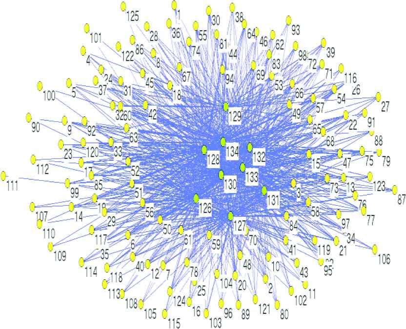
Figures 12 and 13 shows the updated structures of suppliers–manufacturers and manufacturers–packers networks after potential partner discovery respectively. Compared with Figure 10, there are 124 potential manufacturers partners for suppliers are discovered in Figure 12. Similarly, there are 16 potential packers partners for manufacturers are discovered in Figure 13 compared with Figure 11. As we implement that resilience evaluation framework, the
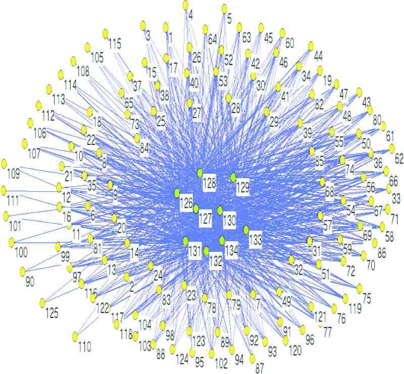
Structure of suppliers–manufacturers after potential partner discovery.

Structure of manufacturers-packers after potential partner discovery.
Figure 14 illustrates the suppliers–manufacturers–packers tripartite supply chain network after discovery of potential partners in the suppliers–manufacturers and manufacturers–packers networks. In the figure, each yellow node represents a supplier, green node symbolizes a manufacturer and red node refers to a packer, the links among the parties refer to their partnerships. To show the effect of the network by fulfilling the discovering task, we take the node labeled 126 as an example, which is a Huawei mobile phone manufacturer and connects with 89 upstream suppliers and 6 downstream packers. There are 534 combinations of supply chain from the suppliers to packers. By implementing the partner discovery process, it is found that 12 suppliers and 1 packers that are nonexistent nodes in the original bipartite networks can be its potential partners. This results in 707 possible combinations, a 32% increase to the original network. From this point, it also implies that the longer the supply chain extends, the more potential supply chains could we have. Furthermore, the connectivity of the tripartite network centered at node 126 increased from 0.647 to 1.176, and the flexibility increased from 0.851 to 1.370, indication great resilience improvement by implementing potential partner discovery. Obviously, the process of discovering potential partners helps the manufacture increase its robustness and reduce the vulnerability when there is a turbulence in the market. It could also enhance the risk response capacity of the supply chain network and ensure the profitability for the participants of the network.
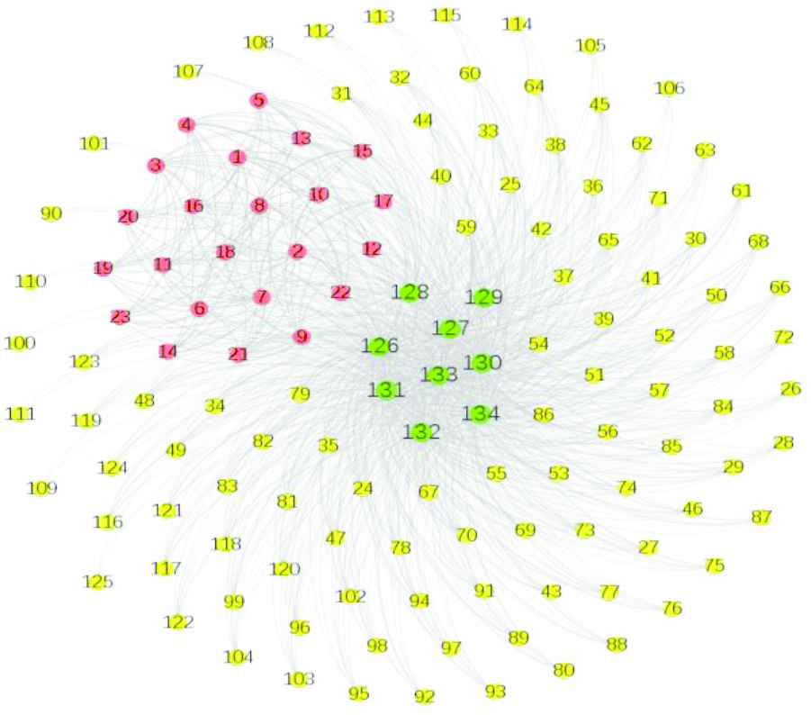
Structure of supply chain network after experiment.
6. CONCLUSIONS
Enterprises that fail to provide necessary supply chain visibility often find too late that interruptions, delays, scrap, risk exposure and quality failures were due to a dangerous reliance on inherent and insufficient supply chain partners. Discovering potential partners in supply chain network helps to improve resilience, visibility and collaboration throughout the partner network. This study proposes a projection-based link prediction approach to discover potential partners in the supply chain network to increase supplier chain resilience and reduce cooperation challenges. The model firstly predicts candidate partnership links based on the supply chain network's structure and its projection one-model graphs. Secondly, it discerns the potential partners by comparing the connectivity of the acquired candidate partnership links with the maximal connectivity of existent partnership links. Thirdly, a resilience evaluation framework is used to assess to what extent that supply chain network's connectivity and flexibility are improved. The application of the model is demonstrated through an experiment of a mobile phone supply chain network. Results of experiment reveals that the proposed algorithm exceeds three other link prediction algorithms in the aspect of AUC index showing higher prediction precision over them. Both connectivity and flexibility are improved in terms of the resilience of the post-discovery network to the original one.
Future research directions on the basic of this paper are as follows:
The proposed potential partner discovery algorithm obtains divides the multi-tier supply chain network into bipartite supply chain networks, which ignores the globality of the supply chain network. Further work will be needed to concentrate on the integrity of the supply chain network.
The proposed model is based on the static supply chain network and ignores the new entrants to the network. Further studies should consider the significance of the supply chain network evolution.
CONFLICT OF INTEREST
The authors declare that they have no competing interests.
AUTHORS' CONTRIBUTIONS
The study was conceived and designed by Zhigang Lu and experiments performed by Qian Chen. All authors read and approved the manuscript.
ACKNOWLEDGMENTS
We thank the financial sponsor from Natural Science Foundation of Shanghai (grant number 18ZR1416900).
REFERENCES
Cite this article
TY  - JOUR
AU  - Zhi-Gang Lu
AU  - Qian Chen
PY  - 2020
DA  - 2020/08/21
TI  - Discovering Potential Partners via Projection-Based Link Prediction in the Supply Chain Network
JO  - International Journal of Computational Intelligence Systems
SP  - 1253
EP  - 1264
VL  - 13
IS  - 1
SN  - 1875-6883
UR  - https://doi.org/10.2991/ijcis.d.200813.001
DO  - 10.2991/ijcis.d.200813.001
ID  - Lu2020
ER  -