
Contextualizing Support Vector Machine Predictions
 , Guy De Tré1,
 - DOI
- 10.2991/ijcis.d.200910.002How to use a DOI?
- Keywords
- Explainable artificial intelligence; Augmented appraisal degrees; Context handling; Support vector machine classification
- Abstract
Classification in artificial intelligence is usually understood as a process whereby several objects are evaluated to predict the class(es) those objects belong to. Aiming to improve the interpretability of predictions resulting from a support vector machine classification process, we explore the use of augmented appraisal degrees to put those predictions in context. A use case, in which the classes of handwritten digits are predicted, illustrates how the interpretability of such predictions is benefitted from their contextualization.
- Copyright
- © 2020 The Authors. Published by Atlantis Press B.V.
- Open Access
- This is an open access article distributed under the CC BY-NC 4.0 license (http://creativecommons.org/licenses/by-nc/4.0/).
1. INTRODUCTION
As the ubiquity of artificial intelligence (AI) grows, computer applications like word processors that translate documents, or videoconference applications that generate transcripts of meetings, are thoroughly satisfying business or user needs. Nevertheless, AI applications like profiling tools that predict capabilities of people without providing any explanation have to be banned in situations where transparency and accountability are mandatory [1,2]. An existing challenge in this regard is to find suitable mechanisms by which the reasons and reasoning behind computer predictions involving complex techniques can be explained with ease [3,4].
To address that challenge in predictions made by a support vector machine (SVM) classification process [5,6], we explore the use of augmented appraisal degrees (AADs) [7] for the contextualization of the evaluations that yield such predictions. Since an AAD has been conceived as a mathematical representation of a connotative meaning in an experience-based evaluation, it can be used for recording not only the level to which an object belongs (or not) to a particular class, but also the object’s features that support that level assignment. Hence, we propose a novel variant of an SVM classification process whereby the resulting predictions are augmented in such a way that those predictions are put in context and an explanation is provided. Our main motivation here is to obtain predictions that expose the aspects deemed to be relevant to the classification.
An important facet of the proposed variant is that, by explicitly representing context, it yields predictions that are better interpretable. Hence, our variant, named explainable SVM classification (XSVMC), can be used within an explainable artificial intelligence (XAI) system [8], by which users can take advantage of such interpretable predictions to make better informed decisions.
A key component of XSVMC is a novel evaluation procedure in which the most influential support vector (MISV) is used for identifying what has been relevant to the classification. This evaluation procedure, which is the main contribution of this work, contextualizes the evaluations in such a way that the forthcoming predictions can be explained with ease.
To describe how XSVMC works, we develop a process whereby handwritten numbers are evaluated to predict the class(es) those handwritten numbers belong to. A visual representation of a resulting prediction is shown in Figure 1: while the left side of this figure shows a handwritten number, which is used as input, the right side of the figure shows a representation of why the proposition “the handwritten number is a ‘3’” is true up to a specific level. The resulting prediction has also been used within an XAI system to produce the following output: “The green part suggests that the drawing is a ‘3’ with a computed grade of
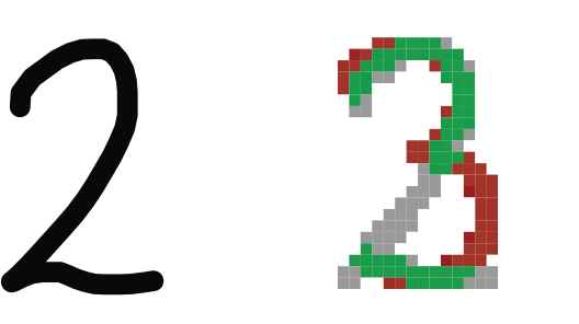
Predicting handwritten numbers.
In the next section, we introduce the AAD concept and briefly describe how it can be integrated into the intuitionistic fuzzy set (IFS) concept. Then, we provide a comprehensive explanation of our novel XSVMC in Section 3 and illustrate in Section 4 how to use it. After that, other existing techniques for explaining individual predictions are reviewed in Section 5. We conclude the paper in Section 6.
2. PRELIMINARIES
As indicated previously, classification in AI is commonly understood as a process in which several objects are evaluated in order to predict the class(es) those objects belong to [9]. In this regard, a classification algorithm can look into the features of an object to evaluate the level to which this object is member of one or more well-known classes Using these evaluations, the algorithm can provide the best evaluated class(es) as a prediction. It is worth mentioning that herein by ‘feature’ is meant a distinctive aspect that is relevant for the classification. For instance, the level of illumination of either one pixel or a group of pixels of the handwritten number shown on the left side of Figure 1 can be deemed to be relevant for the classification of this number.
In situations where an object, say
As shown in Figure 1, the handwritten number can also have features suggesting that it does not belong to the class of handwritten
As noticed above, while a membership grade and an IFS element make it possible to record the level(s) to which an object belongs (or not) to a given class, none of these representations enables the recording of the object’s characteristics that lead to and hence explain this (these) level(s). To record those characteristics, the idea of AADs [7] has been introduced. An AAD of an object
To record the characteristics that indicate why the aforementioned handwritten number should not be a ‘3’, the augmentation of IFS elements with AADs has been proposed [7]. An augmented IFS element, say
3. EXPLAINABLE SVM CLASSIFICATION
As was mentioned earlier, our aim is the contextualization of SVM predictions to make them better interpretable. For that purpose, in this section we describe our novel XSVMC process, by which SVM predictions are augmented with AADs. As depicted in Figure 2, the main components of XSVMC are a learning process, an evaluation process and a prediction step. Among these components, the fundamental contribution of this work is the novel evaluation process that makes use of the MISV to contextualize the evaluations. In what follows we give details of each component.
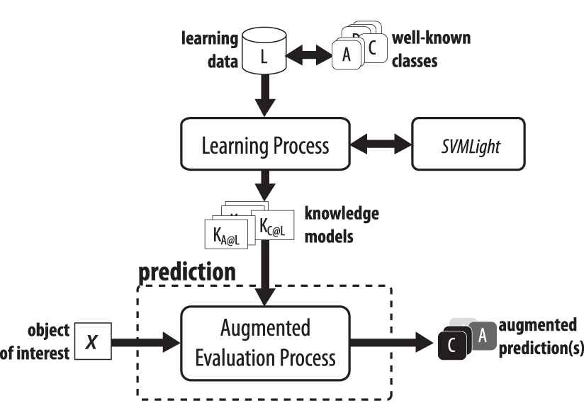
A contextual view of XSVMC [14].
3.1. Learning Process
The aim of the learning process in XSVMC is to obtain a knowledge model for each class in a collection of well-known classes. To describe how it works, we make use of a process that mimics a learning behavior where a person learns about a concept (or class) by studying objects that satisfy or dissatisfy an evaluation criterion related to the concept. The process is based on the feature-influence representational model[15], which is summarized below.
3.1.1. Feature-influence representational model
Let
The overall influence
where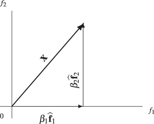 Figure 3
Overall influence of the features of an object x.
A particular knowledge model about
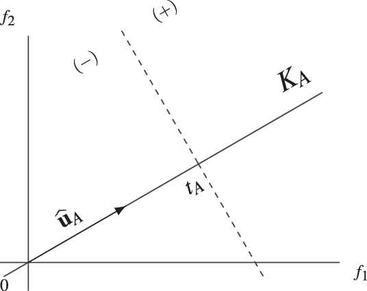 Figure 4
Characterization of a particular knowledge about A.
The specific influence of the features of
where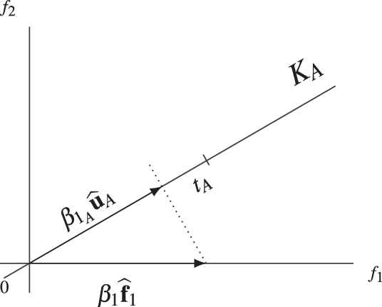 Figure 5
Specific influence of one of the features of x.
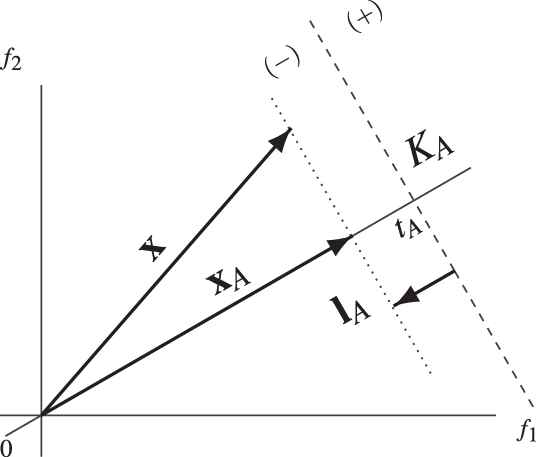
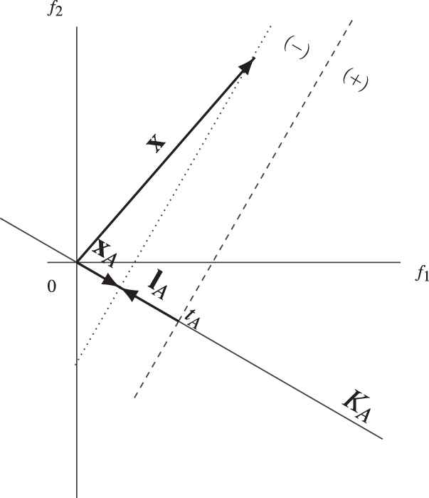
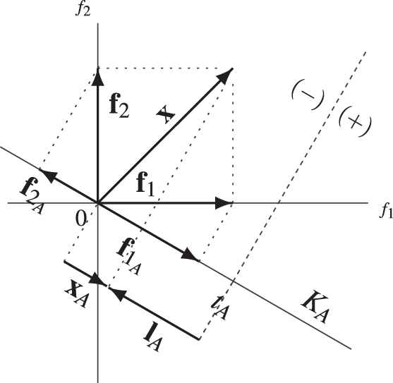
The level to which
i.e, this level is given byIf the directions of
 Figure 6
Resulting specific influence xA of the features of x.
3.1.2. Obtaining knowledge models
At this point, the feature-influence model can be used for explaining how to extract a model of the knowledge about a class
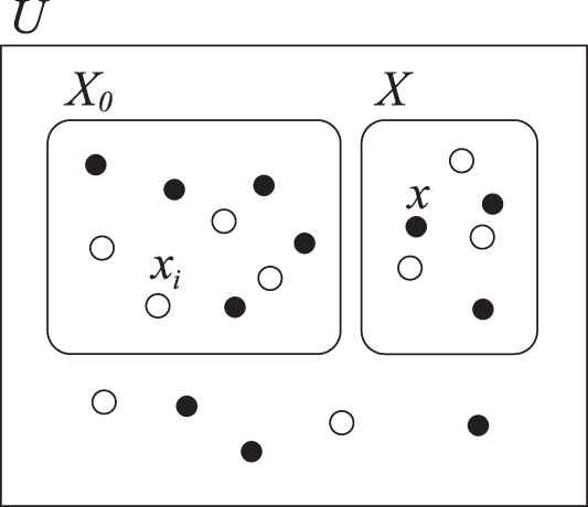
Training and test collections consisting of positive examples, denoted by black circles, and negative examples, denoted by white circles.
For each
Assign an overall importance
Compute
In the first step, the objects’ features that will be considered during the learning process are identified. It is worth mentioning that a feature can represent something about one or more characteristics of an object. For example, a feature can represent the presence of either one pixel or a group of pixels in a digitalized handwritten number.
In the second step, an overall weight for each of the features identified in the first step is assigned based on its relative influence on the classification. For example, the level of illumination can be considered as the overall weight of a feature consisting of one pixel.
In the third step, the components of
Adjusting the component tA of KA.
Adjusting the component ûA of KA.
The problem of finding an optimal couple
Suppose that a hyperplane
The hyperplane
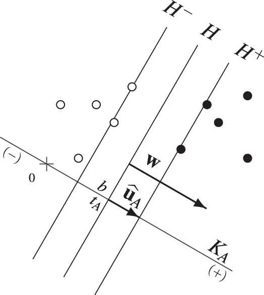
An optimal couple <ûA, tA> in relation to an optimal separating hyperplane H.
To find the values of
The previous problem is reformulated to an equivalent dual problem[16], which consists in finding the Lagrange multipliers such that the gradient of
In this equation,
In situations where the vectors are not linearly separable, those vectors can be mapped to another space in which they can be separated by a linear hyperplane. This means that a vector
Instead of computing the inner product between
Among others, the Polynomial kernel of degree
As noticed, SVMs can be used for the computation of the optimal couple
3.2. Augmented Evaluation Process
A conventional classification algorithm can use the knowledge model resulting from the above-described learning process to evaluate the level to which an object is member of a given class. For example, after obtaining a feature-influence model of the knowledge about class
If a user would like to know in the previous example why the predicted class is
Consider a class
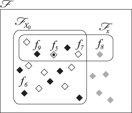
Features collections.
For each feature
For each feature
For each feature
Compute
andrespectively, whereand
It is worth mentioning that (21) and (22) are obtained as follows. Using (2), (3) can be rewritten as
The first term of (25) can be split into the sum of positive specific influences and the sum of negative specific influences. Thus, (25) can be rewritten as
Notice in (26) that, while the sum of positive specific influences will be increased by
The idea behind (21) and (22) is to quantify the levels to which each of the features of
Specific influence of two features, f1 and f2, on the appraisal of a proposition pA: ‘x BELONGS TO A’.
In contrast to a conventional classification algorithm, XSVMC can use the above procedure to perform a contextualized evaluation of the membership (and nonmembership) of an object in a given class. For example, to evaluate the membership of an object
In some situations, the collections
Consider the next variant of (9)
To obtain
To obtain (29) and (30), we split (27) into the sum of positive specific influences and the sum of negative specific influences. Thus, we rewrite (27) as
Notice in (31) that, while the sum of positive specific influences increases if
Notice in (29) that the membership level
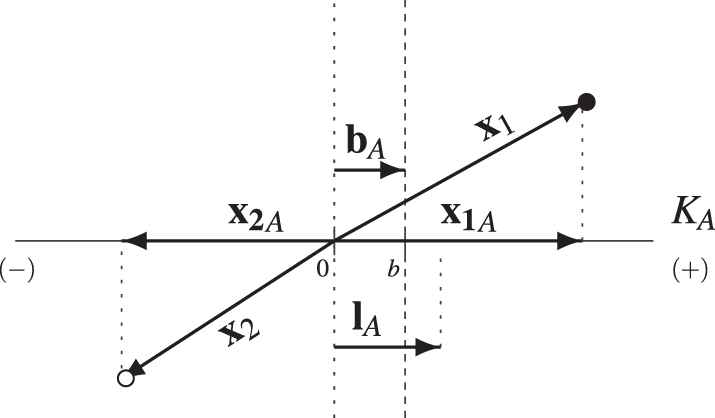
Specific influence of support vectors x1 and x2 on the appraisal of a proposition pA: ‘x BELONGS TO A’.
It is worth mentioning that the main difference between both aforementioned evaluation procedures lies in the strategy to identify which features have been relevant to the evaluation: while the first evaluation procedure makes use of the DV
4. USE CASE
Aiming to illustrate how the novel XSVMC works, in this section we implement a use case where the classes of handwritten digits are predicted. This use case consists of a successful scenario, in which the right class is predicted, and an unsuccessful scenario, in which a wrong class is predicted.
To implement the use case, we use two collections of digitized handwritten numbers: the first one is a very small collection consisting of the handwritten numbers depicted in Figures 14–16, and the second one is the MNIST collection[18], which contains 70000 handwritten numbers.
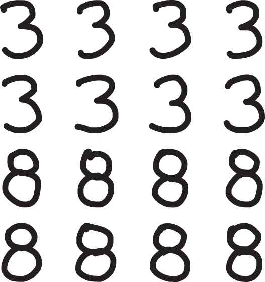
User 1’s training collection (X0@usr1).
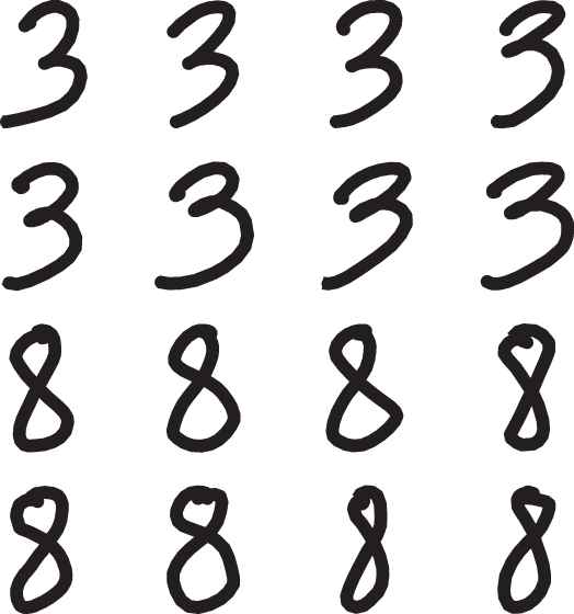
User 2’s training collection (X0@usr2).

User 1’s test collection (X@usr1).
As shown in Figure 17, such a digitized handwritten number consists of
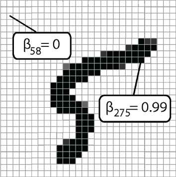
Characterization of a handwritten ‘5’.
To use the learning and evaluation procedures included in XSVMC, each digitized handwritten number has been modeled in a
4.1. XSVMC on a Very Small Collection
An SVM classification process can be effective in cases where the dimension of the feature space
We first use
The results of those contextualized evaluations are listed in Table 1 and Figure 18. Notice in Table 1 that the levels computed with DV are the same levels computed with MISV. This observation makes the equivalence between (21) and (29), as well as the equivalence between (22) and (30) evident. In contrast, the visual representations listed in Figure 18 provide an evidence of the difference between the context of the evaluation obtained with DV and the context of the evaluation obtained with MISV. In these representations, while the green parts suggest that a handwritten number is part of a class, the red part, which a member of the class should have, and the gray part, which a member of the class should not have, indicate that the handwritten number is not part of the class. Notice in this case that, even though a difference between those contexts exists, this difference is rather small.
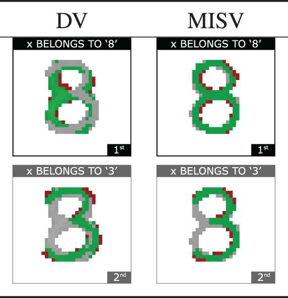
Visual results of the evaluations listed in Table 1.
| DV | MISV | |
|---|---|---|
| 1.4317 | 1.4317 | |
| 1.2104 | 1.2104 | |
| 2.6422 | 2.6422 | |
| 0.5419 | 0.5419 | |
| 0.4581 | 0.4581 | |
| 0.0838 | 0.0838 | |
| 1.2104 | 1.2104 | |
| 1.4317 | 1.4317 | |
| 2.6422 | 2.6422 | |
| 0.4581 | 0.4581 | |
| 0.5419 | 0.5419 | |
| −0.0838 | −0.0838 |
Results of the evaluations of “
A potential explanation for such a small difference is that the DV, which incorporates all the support vectors, and the MISV are substantially similar since the knowledge models used for the previous evaluations have been obtained from a training collection consisting of numbers written only by one person, namely user1.
To obtain further insight in that regard, we use
The results of those evaluations are listed in Table 2 and Figure 19. Notice that the equivalence between (21) and (29), as well as the equivalence between (22) and (30) are also visible in Table 2. Notice also that the difference between the contexts of the evaluations obtained with DV and the contexts of the evaluations obtained with MISV has increased.
| DV | MISV | |
|---|---|---|
| 1.4425 | 1.4425 | |
| 1.2318 | 1.2318 | |
| 2.6743 | 2.6743 | |
| 0.5394 | 0.5394 | |
| 0.4606 | 0.4606 | |
| 0.0788 | 0.0788 | |
| 1.2318 | 1.2318 | |
| 1.4425 | 1.4425 | |
| 2.6743 | 2.6743 | |
| 0.4606 | 0.4606 | |
| 0.5394 | 0.5394 | |
| −0.0788 | −0.0788 |
Results of the evaluations of “
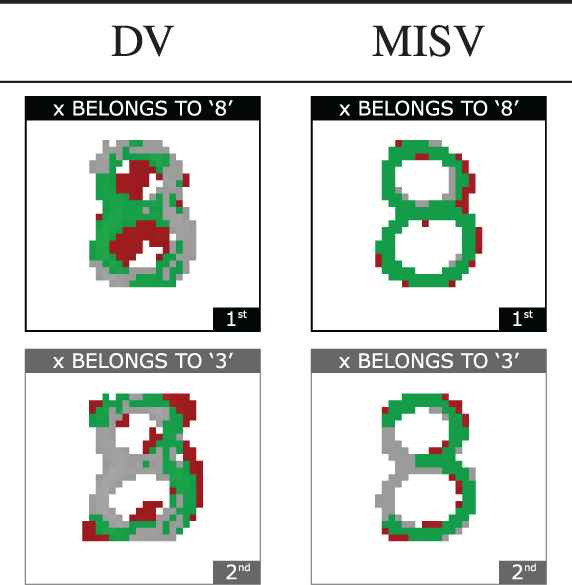
Visual results of the evaluations listed in Table 2.
An explanation for that increment is that in this case the DV incorporates features of the handwritten numbers given by usr2 whose influence differs from the influence of the features included in the MISV, which includes features of one of the handwritten numbers given by usr1. For instance, the influence of the features of the handwritten ‘8”s given by usr2 is reflected in the red part of the visual representation of the evaluation of “
Regarding the prediction of the class the handwritten number
It is worth mentioning that, even though the computed buoyancy is used for sorting the evaluations, it might be considered optional while offering an explanation with a contextualized evaluation. A reason for this it that, compared to the context, the computed buoyancy might have a limited significance for an explanation since the buoyancy could be a very small number – notice in Tables 1 and 2 the effect of scaling the membership levels
4.2. XSVMC on a Large Collection
To illustrate how XSVMC works in cases where the number of samples is greater that the dimension of the feature space
In contrast to the binary classification performed in the previous section, in this section we use XSVMC to perform a multi-class classification of handwritten decimal digits. In this regard, we use an ‘one-versus-the-rest’ strategy to build each of the
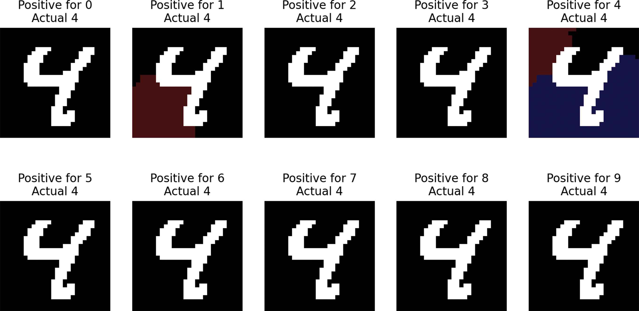
The visual representations of two of those contextualized evaluations are shown in Figure 20. While the first column shows the visual representation of the evaluation of “
Difference between the context of an evaluation based on the directional vector (DV) and the context of an evaluation based on the support vector with the greatest positive influence on the evaluation (MISV).
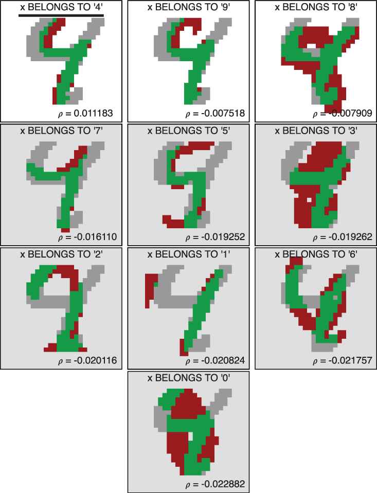
Visual results of the evaluations of the membership and nonmembership of a handwritten ‘4’ in each of the classes of handwritten decimal digits.
An explanation for the difference between the above representations is that in this case the DV incorporates features of several shapes of handwritten numbers ‘8”s whose influence differs from the influence of the features included in the MISV, which is related to the shape of a particular handwritten number ‘8’ – cf. the visual representations listed in Figure 19.
To predict the class of a handwritten number, contextualized evaluations of the membership (and nonmembership) of this number to each of the
| Rank | ||||
|---|---|---|---|---|
| ‘0’ | 0.0181 | 0.0410 | −0.0229 | |
| ‘1’ | 0.0280 | 0.0489 | −0.0209 | |
| ‘2’ | 0.0299 | 0.0500 | −0.0201 | |
| ‘3’ | 0.0434 | 0.0627 | −0.0193 | |
| ‘4’ | 0.1195 | 0.1083 | 0.0112 | |
| ‘5’ | 0.0325 | 0.0518 | −0.0193 | |
| ‘6’ | 0.0180 | 0.0398 | −0.0218 | |
| ‘7’ | 0.0809 | 0.0971 | −0.0162 | |
| ‘8’ | 0.0711 | 0.0790 | −0.0079 | |
| ‘9’ | 0.1487 | 0.1562 | −0.0075 |
Results of the evaluations of the membership and nonmembership of a handwritten ‘4’, denoted by
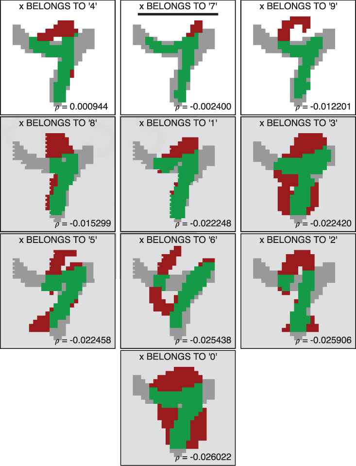
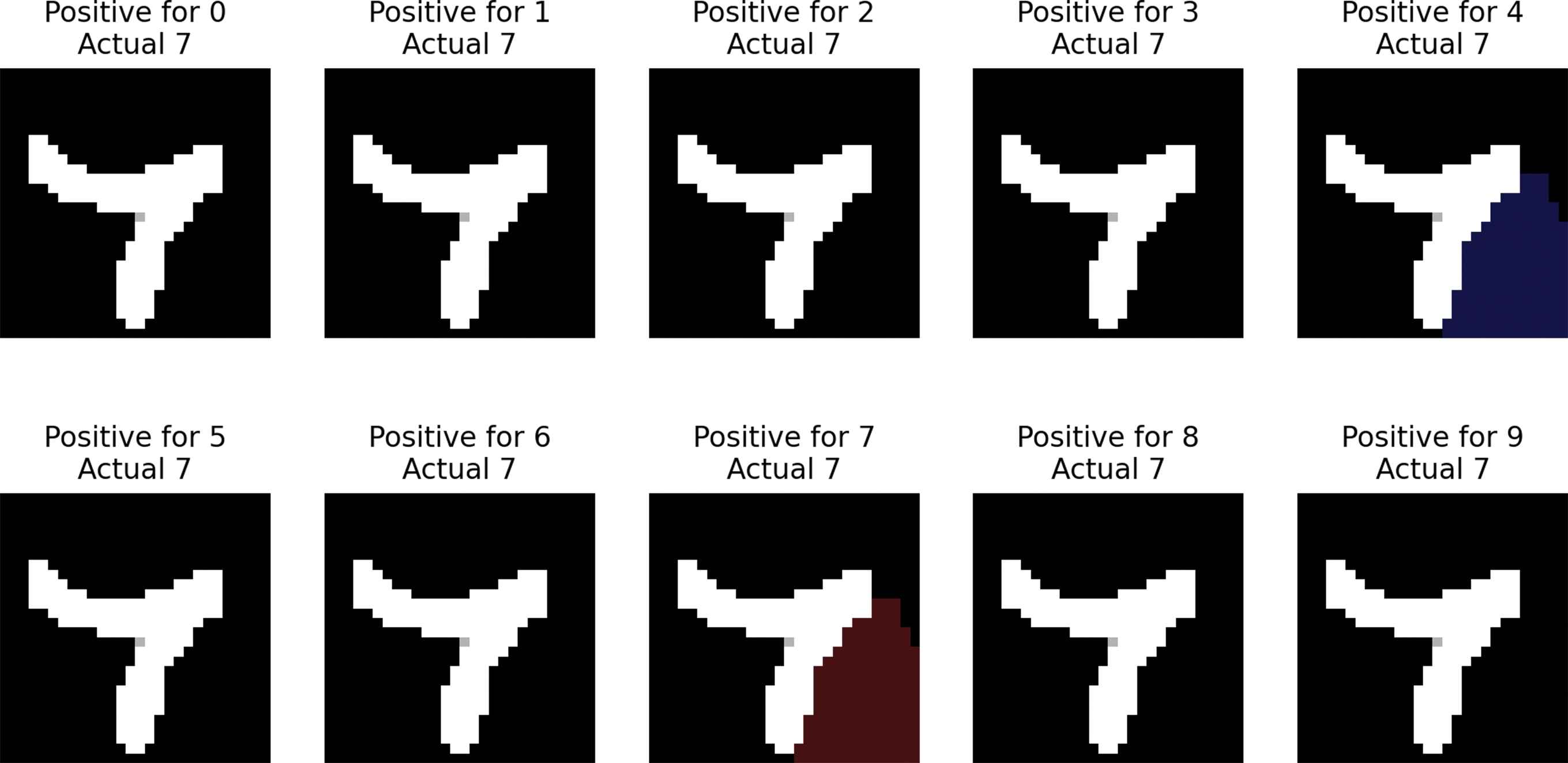
Visual results of the evaluations of the membership and nonmembership of a handwritten ‘7’ in each of the classes of handwritten decimal digits.
The previous results were used as input of an XAI system that incorporates XSVMC to offer the following explanation of the most optimistic prediction: “The green part suggests that your drawing is a ‘4’ with a computed grade of
A potential advantage of XSVMC over a conventional SVM classification process is shown in Table 4 and Figure 22. In this example, a conventional SVM classification process would offer ‘4’ as a prediction since the best evaluated class is ‘4’. In contrast, since XSVMC offers the
| Rank | ||||
|---|---|---|---|---|
| ‘0’ | 0.5056 | 0.0532 | −0.0260 | |
| ‘1’ | 0.0459 | 0.0681 | −0.0222 | |
| ‘2’ | 0.0305 | 0.0564 | −0.0259 | |
| ‘3’ | 0.0445 | 0.0670 | −0.0225 | |
| ‘4’ | 0.1370 | 0.1360 | 0.0010 | |
| ‘5’ | 0.0406 | 0.0630 | −0.0224 | |
| ‘6’ | 0.0231 | 0.0485 | −0.0254 | |
| ‘7’ | 0.1203 | 0.1227 | −0.0024 | |
| ‘8’ | 0.0699 | 0.0852 | −0.0153 | |
| ‘9’ | 0.1750 | 0.1872 | −0.0122 |
Results of the evaluations of the membership and nonmembership of a handwritten ‘7’ in each of the classes of handwritten decimal digits.
To further illustrate the potential advantage of XSVMC over a conventional SVM classification process, we measure the number of right predictions included in the
| Rank | Right Predictions | Freq. Acc. |
|---|---|---|
| 9790 | 9790 | |
| 169 | 9959 | |
| 26 | 9985 | |
| 8 | 9993 | |
| 4 | 9997 | |
| 2 | 9999 | |
| 0 | 9999 | |
| 1 | 10000 | |
| 0 | 10000 | |
| 0 | 10000 |
Number of right predictions according to the ranking of the
It is worth mentioning that in situations where only the best evaluated class is presented as the most optimistic prediction, a conventional SVM classification process and an XSVMC process have the same performance. To prove that, the test collection of
| Kernel | Error Rate |
|
|---|---|---|
| XSVM | SVM | |
| 8.19% | 8.19% | |
| 8.07% | 8.07% | |
| 2.46% | 2.46% | |
| 2.10% | 2.10% | |
| 2.11% | 2.11% | |
| 2.85% | 2.85% | |
XSVMC versus Conventional SVM classification.
4.3. XSVMC versus Alternative Approaches
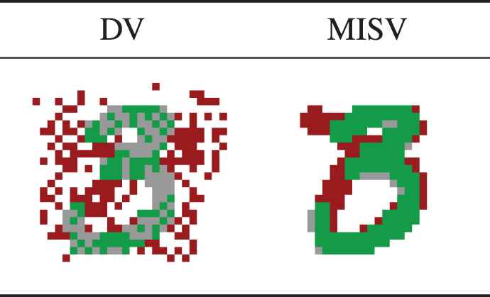
To illustrate potential advantages of XSVMC over alternative approaches, we use LIME [20] and ABELE [21] to perform the evaluations of the handwritten numbers considered in Figures 21 and 22.
Visual results of the evaluation of the handwritten number ‘4’ depicted in Figure 21 using LIME.
Visual results of the evaluation of the handwritten number ‘7’ depicted in Figure 22 using LIME.
LIME is a technique that tries to explain a prediction made by a classifier through an interpretable local model that is built around the prediction without knowing the details of the classifier. To produce the visual representations depicted in Figures 23 and 24, we use the source code of LIME (which is available in https://github.com/marcotcr/lime) with the same configuration of the SVM classifier used in Figures 21 and 22 (i.e., a polynomial kernel
Regarding ABELE, it is an extension of LORE [22] that, in a similar way to LIME, tries to explain a prediction by building an interpretable local classifier with a synthetic neighborhood of the handwritten number under evaluation, but, in addition, it takes into account existing relationships between the pixels of the handwritten number for building the synthetic neighborhood. To produce the visual representations depicted in Figure 25, we use the source code of ABELE (which is available in https://github.com/riccotti/ABELE) with the implemented Random Forest [23] classifier. Notice that, in comparison to LIME, the visual representations produced with ABELE show more clearly the approximations of what has been relevant to the classifier. However, ABELE needs more computational resources than LIME while evaluating all the generated synthetic samples.

Visual results of the evaluation of the handwritten numbers ‘4’ and ‘7’ depicted in Figures 21 and 22 respectively using ABELE.
5. RELATED WORK
An extensive survey of methods proposed for explaining computers predictions is presented in the work of Guidotti et al. [24]. In that survey, two main strategies have been identified: one is about the design of “transparent algorithms” that produce interpretable predictions, and the other is concerned with the interpretation of predictions without knowing the details of the algorithms that yield such predictions.
One of the methods aiming to interpret (and understand) predictions without knowing the internal details is a method proposed for decomposing a nonlinear image classification decision [25]. That method produces a heat map that highlights the relevant pixels, i.e., the pixels that have a significant influence on the classification decision. Another example is an explanation technique which tries to explain the predictions made by unknown classifiers by building interpretable local models that mimic the behavior of such classifiers [20]. In a similar way, the method proposed in the work of Baehrens et al. tries to extract a local model consisting of “explanation vectors,” which contain features that are relevant to a given prediction [26]. The visualization method proposed by Zeiler and Fergus also tries to interpret the influence of the features (pixels) and the behavior of a specific knowledge model [27].
A particularity about the aforementioned methods is that they try to identify what has been relevant to the classification decision after a prediction is made. In contrast, XSVMC identifies what has been relevant before the prediction. This aspect is deemed to be a key advantage since the influence of the features can be taken into account to guide the classification decision. In this regard, XSVMC can be considered to be part of the “transparent algorithms” identified by the above-mentioned survey. The method proposed by Loor and De Tré to contextualize naive Bayes predictions [28] is another example of such transparent algorithms.
A classification process that generates visual explanations has been proposed by Hendricks et al. [29]. In that process, images with annotated features are used as input to train an explanation model that combines classification and sentence generation in natural language. The process yields sentences including discriminative features that justify why an object belongs to the predicted class. However, such sentences do not include features justifying why the object does not belong to the class as XSVMC does.
The contributions made by the fuzzy logic community to the development of the explainable AI research field have been analyzed by Alonso et al. [30]. The results of that work suggest that the contributions made by the fuzzy logic community seem to be distant with the efforts made by the non-fuzzy community. However, that study suggests that those contributions can be linked to address the challenges arising in that field. In this regard, while potential options to develop XAI systems with fuzzy modeling have been proposed by Mencar and Alonso [31], non-fuzzy options have been proposed by Adadi and Berrada [32].
6. CONCLUSIONS
In this paper, we have proposed a novel variant of an SVM classification process by which the resulting predictions are contextualized in order to improve their interpretability. In the proposed variant, named XSVMC, the membership and nonmembership of an object in a particular class are evaluated in such a way that the context of the evaluation is explicitly recorded. Hence, predictions resulting from such contextualized evaluations can be explained with ease. In this regard, a key component of XSVMC is a novel evaluation method that makes use of the MISV to contextualize the evaluations.
An important aspect of XSVMC is that users can take advantage of such contextualized predictions to give preference to the class(es) with the best credible justification. We have illustrated this aspect through the implementation of a use case where the classes of handwritten numbers are predicted.
Even though the results of the aforementioned implementation suggest that the contextualization of SVM predictions can favor the interpretability of them, qualitative attributes like coherence, naturalness and clearness that might be perceived by a person on those predictions are still subject to validation. In this regard, studies oriented to conduct such validations are considered (and suggested) as future work.
CONFLICT OF INTEREST
None.
AUTHORS' CONTRIBUTION
Marcelo Loor, main author Guy De Tré, PhD thesis promoter, advisor.
FUNDING STATEMENT
This research received funding from the Flemish Government under the “Onderzoeksprogramma Artificiële Intelligentie (AI) Vlaanderen” programme.
ACKNOWLEDGMENTS
The authors acknowledge the valuable and insightful comments given by the anonymous reviewers. The authors are also very grateful to the persons who have written the numbers contained in the small collection used in Section 4.1.
Footnotes
This paper is an extended version of the work published in Marcelo Loor and Guy De Tré. Explaining Computer Predictions with Augmented Appraisal Degrees. Proceedings of the 11th Conference of the European Society for Fuzzy Logic and Technology (EUSFLAT 2019), pages 158–165. Atlantis Press, 2019/08. https://doi.org/10.2991/eusflat-19.2019.24
In this example, one can also say that
REFERENCES
Cite this article
TY  - JOUR
AU  - Marcelo Loor
AU  - Guy De Tré
PY  - 2020
DA  - 2020/09/22
TI  - Contextualizing Support Vector Machine Predictions
JO  - International Journal of Computational Intelligence Systems
SP  - 1483
EP  - 1497
VL  - 13
IS  - 1
SN  - 1875-6883
UR  - https://doi.org/10.2991/ijcis.d.200910.002
DO  - 10.2991/ijcis.d.200910.002
ID  - Loor2020
ER  -