
A New Approach for Low-Dimensional Constrained Engineering Design Optimization Using Design and Analysis of Simulation Experiments
 , Ratchatin Chancharoen2, , Gridsada Phanomchoeng2, Lunchakorn Wuttisittikulkij1, *
- DOI
- 10.2991/ijcis.d.201014.001How to use a DOI?
- Keywords
- Constrained optimization; Surrogates; Kriging; Computationally expensive function; Global optimization
- Abstract
The number of function evaluations in many industrial applications of simulation-based optimization problems is strictly limited. Therefore, only little analytical information on objective and constraint functions is available. This paper presents an adaptive algorithm called the Surrogate-Based Constrained Global-Optimization (SCGO) method to solve black-box constrained simulation-based optimization problems involving computationally expensive objective function and inequality constraints. Firstly, Kriging surrogate is constructed over a new overall objective function (called loss function) to approximate the behavior of a true model. Then, an adaptive approach is provided to improve the optimal results sequentially while enforcing a feasible solution. The SCGO method is tested on several classical engineering design problems namely design of a tension/compression spring, design of a welded beam, design of a pressure vessel, and three-bar truss design. The results demonstrate that SCGO has advantages in solving the costly constrained problems and needs less costly function evaluations. Optimization results prove that the proposed algorithm is very competitive compared to the state-of-the-art metaheuristic algorithms.
- Copyright
- © 2020 The Authors. Published by Atlantis Press B.V.
- Open Access
- This is an open access article distributed under the CC BY-NC 4.0 license (http://creativecommons.org/licenses/by-nc/4.0/).
1. INTRODUCTION
Optimization technologies have been extensively applied in engineering design problems to improve the design quality and shorten the design cycle. In engineering and mathematics, optimization problems based on mathematical characteristics consist of three basic elements including (i) an objective function that needs to be minimized or maximized, (ii) constraints that are relations between decision variables and the parameters, (iii) the set of controllable inputs (decision variables) which affects the value of the objective function. In an optimization problem, the types of mathematical relationships between the objective and constraints and the decision variables determine how difficult it is to solve, the solution methods or algorithms that can be used for optimization, and the assurance of the optimality of the solution. Optimization problems can be categorized into many classes depending on the linearity of the objective function, the modality of the objective function, the number of objective functions, the availability of constraints, the number of decision variables, and the linearity of the constraints (discrete or continuous). A general optimization problem is usually described as a combination of these classifications, see [1]. Generally, the term optimization means to find the best levels of design variables set (
For the past decades, lots of practical engineers and scientists have not trusted expensive model-based optimization methods to obtain designs [21]. As opposed to the algebraic model-based models, surrogate-assisted simulation-optimization does not assume that an algebraic description of the true model is available. However, the model may be available as a black-box that only allows the approximation of the objective and constraints as input/output sets of data. Also, many large-scale and/or detailed true-models may be time-consuming to run [22–26]. To overcome such difficulties, researchers have applied surrogate-based learning methods (e.g., polynomial regression, Kriging, and radial basis function) [18,27,28]. Surrogate-based methods can “learn” the problem behaviors and approximate the function values. These approximation models can speed up the function evaluation and the estimation of the function value with acceptable accuracy. Besides, they can improve the optimization performance and provide a better final solution. Various types of real-world engineering optimization problems have been solved by applying surrogate-based methods such as dynamic and stochastic control system design, sub-communities in machine learning problems, discrete event systems (e.g., queues, operations, and networks), manufacturing, medicine and biology, engineering, computer science, electronics, transportation, and logistics, see [17–19,25,29,30]. Several studies have systematically illustrated the advantages of surrogate-based optimization algorithms [18,21,23,31].
1.1. Related Works
A complex engineering model often takes several or more hours to run a single simulation. Also, design problems in engineering applications as described by the simulation models, are always “black-box” [32]. The search in constraint black-box optimization is difficult since there is not usually a priori knowledge about the feasible region and the fitness landscape. This problem becomes more complex when only a limited number of function evaluations are allowed to be used in the search. The area of efficient constrained optimization is optimization under a severely limited budget of fewer than 1000 functions [33]. Due to the high-computational overhead and the unknown function expressions, common optimization algorithms including Whale Optimization Algorithm (WOA) [11], Grey Wolf Optimizer (GWO) [10], Gravitational Search Algorithm (GSA) [34], Salp Swarm Algorithm (SSA) [35], Co-evolutionary Particle Swarm Optimization (CPSO) [36], Grasshopper Optimization Algorithm (GOA) [37], and Ant Lion Optimizer (ALO) [12] are very expensive if they are directly implemented on these computationally expensive models. For instance, these algorithms require 4,000–18,000 function evaluations to solve the classical constrained engineering design problems namely design of a tension/compression spring, design of a welded beam, design of a pressure vessel, and three-bar truss design. The most common way to incorporate constraints into the mentioned metaheuristics is to employ penalty functions [38,39]. There are also several other approaches available for constraint handling, see review on constraint optimization presented by [38,40,41].
These real-world applications commonly belong to the class of black-box simulation-optimization problems. The state-of-the-art in handling complex and costly problems arising from real-world applications using surrogate models in optimization is reviewed in [3,17–20]. The Efficient Global Optimization (EGO) algorithm was first introduced by [42] that used surrogate models (mostly Kriging) through maximizing Expected Improvement (EI) criterion. This algorithm has been developed in different studies, see [43–45]. Also, the probability of improvement [46], the generalized EI [47], and the augmented EI [48] have been also proposed to adaptively determine the next sampling point in Kriging-based optimizations. A surrogate-based gradient-free optimization algorithm has been developed in [32] that can handle the optimization problems including nonlinear equality or inequality constraints, where the function evaluations are expensive. A surrogate-based PSO method to solve structural design optimization problems with expensive constraint functions has been presented in [49]. RBF-assisted evolutionary programming algorithm to solve high-dimensional problems with the black-box objective and inequality constraints has been developed in [32,33,50]. Simpson et al. summarized the use of each metamodel. RSM is well established, easy-to-use, and suitable for low dimensions. Neural Network metamodel is more suitable for highly nonlinear problems and is recommended for deterministic applications. Kriging metamodel is suitable for low dimension and it is flexible regarding employing different correlation functions [17,51]. Many Kriging-assisted efficient optimizers have been developed in the last years [52–54]. However, Kriging's performance is well confirmed in low-dimensional problems regarding the scope of the current study, see [23,28,55,56].
1.2. Problem Statement
Regarding the limitations found in existed common constrained optimization studies, this study consists of three main contributions as follows:
Most optimization algorithms need to set their parameters concerning the specific optimization problem to show good performance. In other words, it has been necessary for such methods to carefully adjust the parameters of the algorithm to each problem. In real black-box optimization, all these adjustments would probably require knowledge of the problem or several executions of the optimization code [33]. There are different parameters that have been manually adjusted in [57–59] such as distance requirement cycle, constraint normalization, random start probability, and logarithmic transformation of the fitness function, see [33]. The first contribution of the current study is to present the algorithm which does not need manual adjustment of the mentioned parameters to the problem at hand.
Generally, sequential sampling methods are used to iteratively update the surrogate and improve the solution found during the optimization process. These methods iteratively refit the surrogate to improve the best solution so far during the optimization process. However, the updating procedure increases computational time-consumption. Moreover, one of the main contributions of the proposed algorithm is that only one surrogate is fit on the initial training sample points, and there is no need to refine the surrogate sequentially.
Various surrogate-based optimization algorithms are developed to solve problems with expensive simulations. However, deciding on the suitability of the surrogate model to be incorporated within a constrained optimization model remains an open challenge [21,26,60]. There is also a lack of studies in the literature that compare the performances of surrogate's application and metaheuristics in the same platforms of constrained optimization problems. The proposed method is developed to employ the small number of function evaluations as well as to keep the accuracy of the optimal results (lower objective function value) as compared to some state-of-the-art metaheuristic algorithms through the same four platforms of constrained engineering design problems.
This paper aims to develop an effective search algorithm based on surrogate applied in the optimization of expensive simulation models (i.e., with costly function evaluation). This paper limits its focus to low-dimensional (small-scale) constrained optimization models with less than five design variables with a single objective. Space-filling design methods such as Latin Hypercube Sampling (LHS) and Grid Design (GD) [61,62] are employed to construct both training and search sample points. A new overall loss function is introduced by integrating the normalized single objective and constraints of the optimization model. Then, one surrogate is constructed on this overall loss function. This surrogate can be effectively used to create cheaper outputs using larger sample points to speed up the search of the global optimum with a limited number of function evaluations and less computational time. Using sorted grid points, the relevant true model's output is computed and the best feasible point is obtained. Then, an adaptive improvement approach is derived to sequentially improve the obtained solution and reach an optimal point.
The rest of this paper is organized as follows: Section 3 describes the proposed approach developed in this study. Test problems for constrained engineering design problems in the mathematical structure and their experimental results are presented in Section 3. Section 4 provides more discussions for the obtained results. Finally, this study is concluded in Section 5.
2. PROPOSED ALGORITHM
In this section, the proposed approach namely Surrogate-Based Constrained Global-Optimization (SCGO) is described which solves the constrained optimization problem.
2.1. Algorithmic Framework
Figure 1 sketched the flow diagram of the proposed SCGO approach. The main steps involved in the proposed algorithm proceed in the following steps. Also, the pseudocode of SCGO is presented in Algorithm 1.
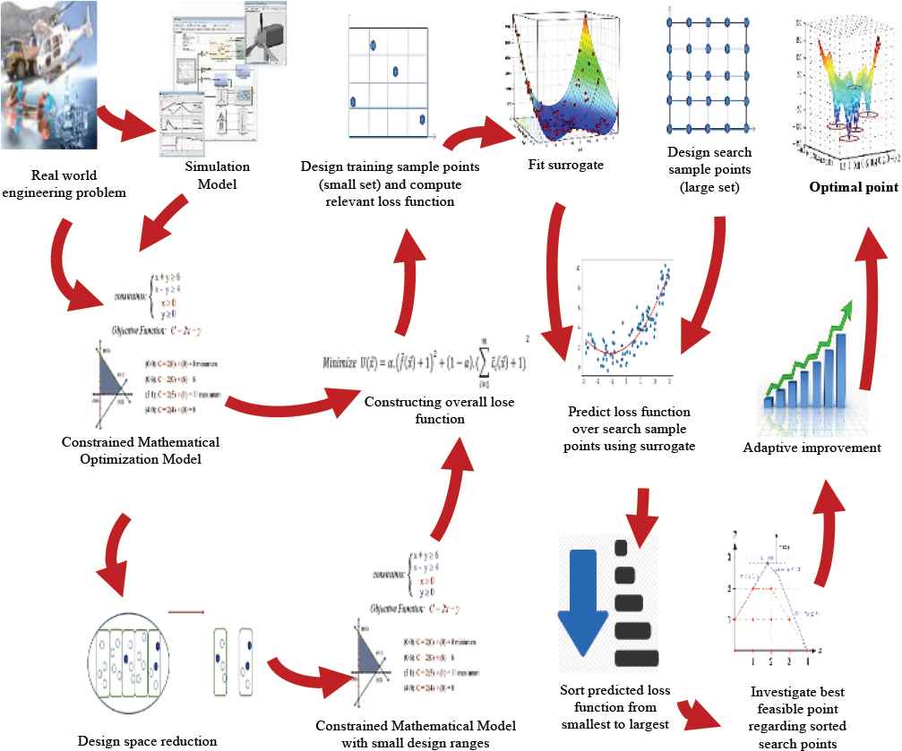
The procedure of proposed Surrogate-Based Constrained Global-Optimization (SCGO) approach.
Step 1:Design training sample points
In this paper, the SCGO algorithm is developed for the low-dimensional (i.e., less than four variables) and expensive problems. For such problems, it has been recommended to design 30 training points as a small sample set or 100 training points as a large sample set using space-filling approaches (e.g., LHS, GD), see [56,65]. The space-filling approach can treat all the regions of design space equally. LHS has been commonly defined for designing sample points based on the space-filling concept [66,67]. Undoubtedly, the simplest and the most popular sampling design methods utilize LHS [17,18].
Algorithm 1: Proposed SCGO algorithm in pseudocode.
Input: Objective function
Output: The optimal solution
1: begin
2: Design initial training sample points using space-filling design (e.g. LHS) with dimension
3: Run the simulation model and obtain
4: Normalize objective function to
5: Normalize all constraint functions to
6: Compute overall loss function
7: Put
8: Design search sample points using grid sampling design with dimension
9: Run Kriging and predict
10: Sort
11: Set
12: while (obtain
►
13: Run simulation model for first point in set of sorted
14: if (point is feasible) then
15:
16: else if
17: Run simulation model for the next point in set of sorted
18: end if
19: end while
20: for (all
21: Run adaptive improvement
► see Algorithm 2.
22:
23: end for
24: return
25: end algorithm
Three common choices are available to ensure appropriate space-filling of the sample points in LHS design namely minimax, maximin, and desired correlation matrix, see [28]. The GD design can fill the whole design space like LHS and has the strength to allocate points in each corner of the design space. The GD was adapted to balance discrete experimental factors in a continuous space [68]. In this study, two Matlab® functions namely “lhsamp” and “gridsamp” in the DACE toolbox are used to design the required sample points.
Step 2: Run the true model and collect the model's outputs
Regarding the designed training sample points in the previous step, the true model (constrained mathematical model) is run and relevant outputs are computed for the objective function, and each constraint function separately.
Step 3: Compute overall loss function
To define an overall function to be used in search of an optimal feasible point, an overall loss function is proposed by the following equation:
This loss function is computed for each training sample point (input combination) using collected outputs from Step 2 in the objective function and constraints. In this loss function, the weight factor
Step 4: Fit a Kriging surrogate
In this step, a Kriging surrogate is fitted on computed input/output data in previous steps (designed training sample points by space-filling design and overall loss function). In a Kriging model, a combination of a polynomial model and realization of a stationary point is assumed by the form of
Step 5: Design search sample points
One of the simplest approaches to the optimization method to search for optimal solutions by employing surrogate instead of an expensive original model is the “grid-search” method. In this approach, the whole design space (exploration) is investigated through the evaluation model components consisting of objectives and constraints sets in the equally spaced grid points [72]. Also, the grid points can be replaced with random points, which are spread in the whole design space (Monte Carlo random search) or with some other space-filling methods. In this searching method, there is a chance to find the global optimum solution because searching is not bounded to the local valley [23]. Here, a space-filling design method is used to produce two groups of sample points including training samples and search sample points. Training sample points are used for constructing surrogates (see Step 1). Search sample points are used to investigate the optimal feasible points. In the search procedure, the surrogate is run instead of the original constrained optimization model. Therefore, a greater set of sample points does not imply a computationally expensive task. Moreover, the greater set of sample points can be designed by a space-filling design method to derive the search procedures.
Step 6: Approximate sorted loss function values
In this step, the fitted Kriging surrogate (Step 4) is used to approximate the loss function values for each designed search sample point (Step 5). Then these values are sorted from smallest to largest.
Step 7: Search optimal feasible points
Regarding the sorted search points that are arranged from the smallest to the largest predicted loss values (see Step 6), the original true model (here mathematical constrained optimization model) is run and the relevant values of the constraint functions are obtained. It starts from the smallest predicted loss value. All the infeasible points are removed from the list of candidacy (i.e., death penalty method for constraint handling, see [38]). For the first obtained feasible point, the relevant objective value is computed. Here, the three first best feasible points are considered to derive adaptive procedure on them as elucidated in the next step.
Step 8: Derive adaptive improvement procedure on the best feasible points
Sometimes, due to the low correlation between the predicted optimum point (which is estimated by surrogate) and the other points, the surrogate does not show enough accuracy in the optimal point as compared to the original model. For instance, Figure 2 shows a shifting predicted optimal point comparing with a true optimum point in an original model for a problem with two input variables. It means that the surrogate is not able to detect the location of the true optimum point when no points are sampled around the true optimum point. The appropriate updating procedure needs to be done to improve the optimal result sequentially, particularly around the predicted optimum points. This is obtained by adding new neighbor points around the current best point. However, to find the neighbor points around the current best point, different strategies of sampling design can be employed (e.g., full factorial design, fractional factorial design, etc.). For models with a small number of design variables (low-dimensional constrained optimization problem), two-level full factorial and fractional factorial designs have been recommended [73,74] to define
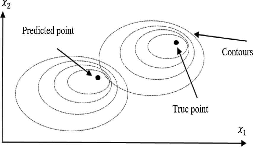
True optimum versus predicted optimum with surrogate for design space with two variables.
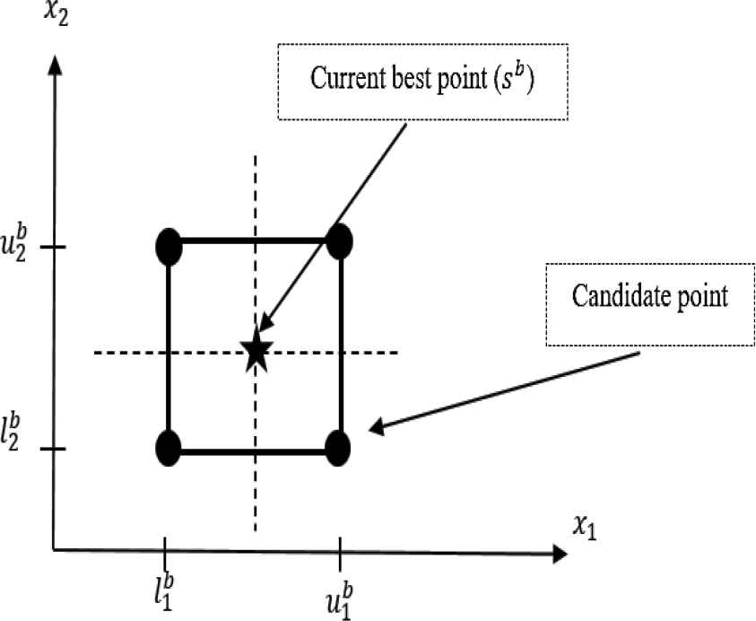
Four candidate points around current best point based on the two-level full factorial design for problem with two design variables.
Algorithm 2: Adaptive improvement in pseudocode.
Input: The best feasible point
Output: The improved best feasible point
1: begin
2: for
3: for
4: while
5: Define/redefine the weight scale
► manually or randomly
6:
7:
8: end while
9: Run simulation model over
10: if
11:
12: else if
13:
14: end if
15:
16: end for
17: if (all members in
18: break
► return to line 2 and redefine
19: end if
20:
21:
22: end for
23:
24: Return
25: end algorithm
2.2. Space Reduction Procedure (If Needed)
For a surrogate model to be useful in an optimization context, the surrogate model must be accurate at the sequence of iterates generated by the search algorithm as it converges towards the true optimum. In the cases with wide design space, first, the size of the design space needs to be reduced to a smaller region of interest to allow for a more accurate surrogate model to be generated. Different algorithms have been developed for design space reduction such as variable-fidelity framework with design space reduction [75], a rough set method [76], and domain optimization algorithm [77]. Moreover, in such problems with wide design space, to gain more accuracy in the constructed surrogate, a design space in a smaller region needs to be reduced first. This pre-optimization procedure is performed before the main optimization procedure regarding Algorithm 1. The proposed design space reduction algorithm proceeds as follows:
Step 1: Design the experiments (using space-filling design method) for the original range of design space.
Step 2: Obtain the true model's output for the objective function and each constraint for designed sample points in the previous step.
Step 3: Fit a surrogate for input/output data for objective and one surrogate for each constraint separately (i.e. polynomial regression can be used as a cheaper surrogate than Kriging).
Step 4: Derive optimization procedure and obtain the best feasible point using common optimization methods (e.g. genetic algorithm or particle swarm optimization).
Step 5: Improve the result using an adaptive improvement procedure for the obtained best feasible point from the previous step and gain a rough optimum point.
Step 6: Define the smaller region of design space (compute the upper and the lower bounds) by
3. TEST OF THE SCGO METHOD IN ENGINEERING APPLICATION
In this section, four real-world constrained engineering design problems namely tension/compression spring, pressure vessel designs, welded beam, and three-bar truss design are employed to investigate the performance of the proposed method. Note that all of the four problems are performed in Matlab® environment. In the following, these test problems and given results using the proposed SCGO method are explained in detail.
3.1. Tension-Compression Spring Design
A tension-compression spring design problem is described in [78]. In this problem, the objective is to minimize the weight of a spring
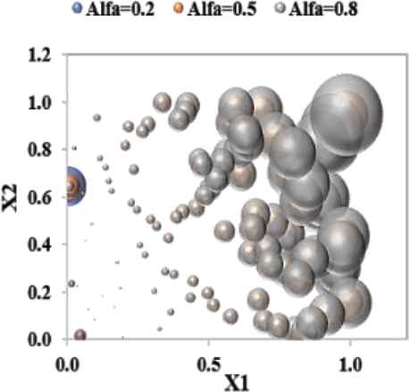
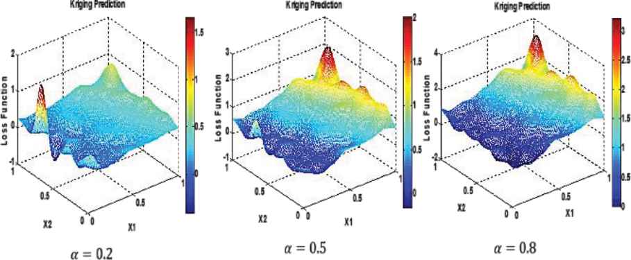
This constrained optimization problem has been solved by the SCGO proposed method in this paper. In the steps of the problem-solving procedure, first, the training set is designed with the size of 30 sample points using the space-filling design (e.g., LHS, see [65]). Then, for each sample point and regarding Equation (3), the overall loss function is computed for three different values of
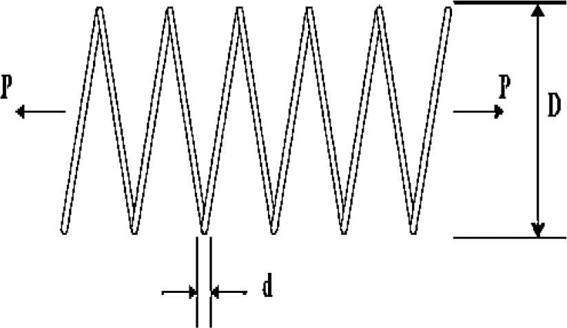
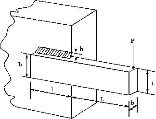
Schematic overview of tension/compression spring.
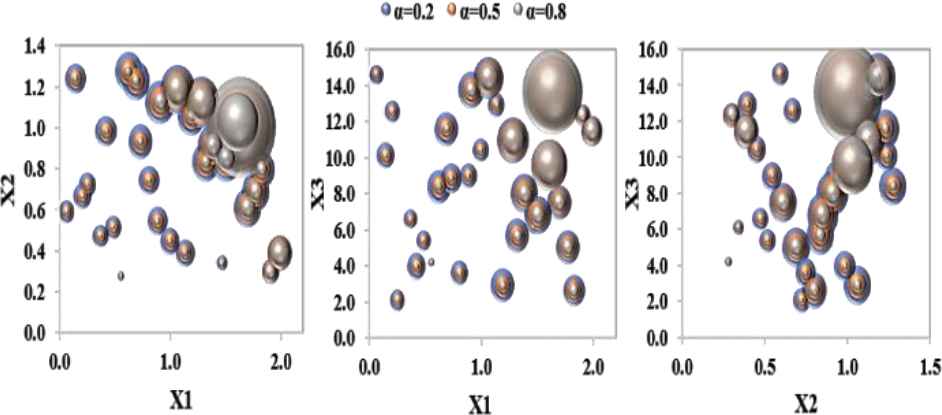
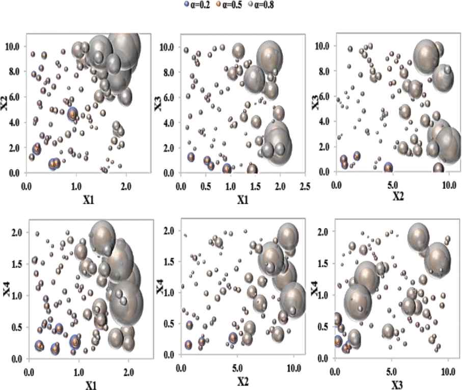
Magnitudes of loss functions over training sample points for two design variables in tension-compression spring design problem.
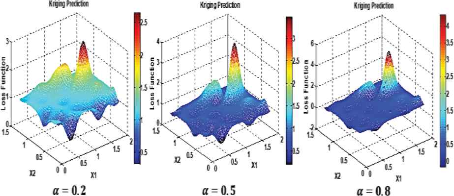
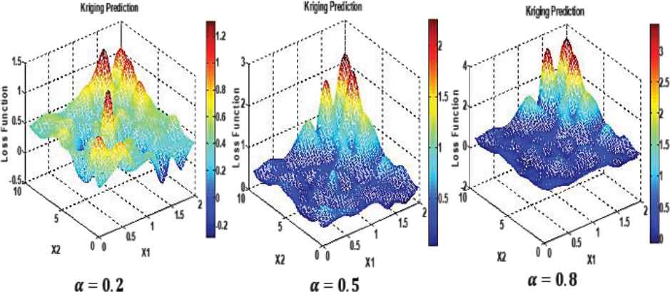
Surface plots of Kriging surrogate fitted over training points and loss functions for two design variables in tension-compression spring design problem.
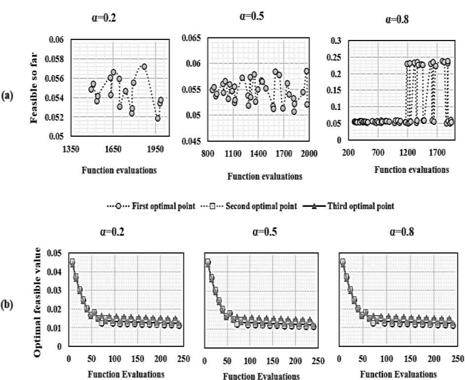
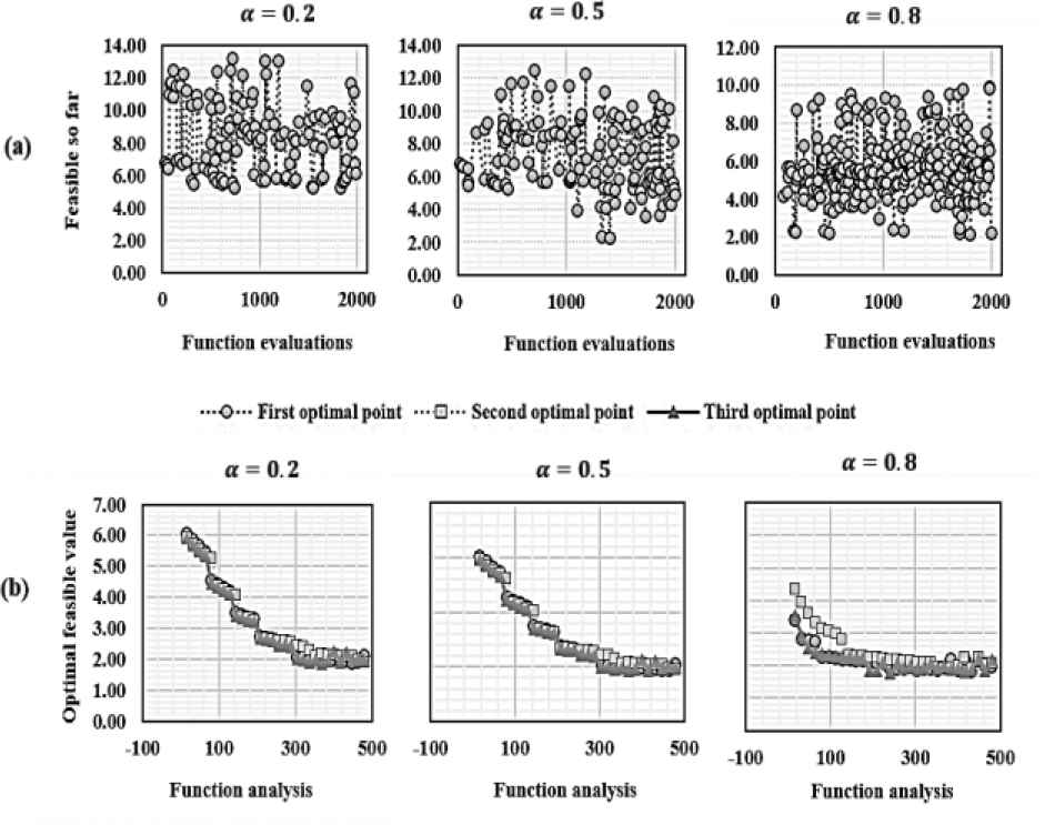
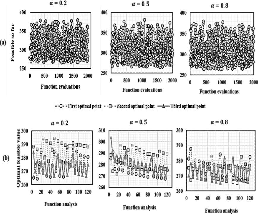
(a) Feasible points regarding sorted grid points (search sample points) and (b) adaptive improvement for three optimal points obtained from sorted grid points in tension-compression spring design problem.
| Algorithm | Optimum Variables |
Optimal Weight | Function Evaluations | |||
|---|---|---|---|---|---|---|
| X1 | X2 | X3 | ||||
| SCGO | α = 0.2 | 0.05074 | 0.36608 | 9.85518 | 0.011172 | 1763 |
| α = 0.5 | 0.05074 | 0.36608 | 9.85518 | 0.011172 | 1125 | |
| α = 0.8 | 0.05074 | 0.36608 | 9.85518 | 0.011172 | 571 | |
| GWO | 0.05169 | 0.35674 | 11.28885 | 0.012666 | --- | |
| WOA | 0.05121 | 0.34522 | 12.00403 | 0.012676 | 4410 | |
| GSA | 0.05028 | 0.32368 | 13.52541 | 0.012702 | 4980 | |
| SSA | 0.05121 | 0.34522 | 12.00403 | 0.012676 | --- | |
| CPSO | 0.05173 | 0.35764 | 11.24454 | 0.012675 | 5460 | |
SCGO, Surrogate-Based Constrained Global-Optimization; WOA, Whale Optimization Algorithm; GWO, Grey Wolf Optimizer; GSA, Gravitational Search Algorithm; SSA, Salp Swarm Algorithm; CPSO, Co-evolutionary Particle Swarm Optimization.
Comparison of SCGO optimization results with literature for the tension-compression spring design problem.
3.2. Welded Beam Design
A welded beam is designed for minimum fabrication cost subject to constraints on shear stress (
Schematic overview of welded beam design problem.
To solve this constrained optimization problem with the proposed SCGO algorithm, the training sample points is designed with a size of 100 points. Figure 9 illustrates the magnitudes of the overall loss function in the set of training points. The optimization procedure is the same as for the previous problem, the Kriging surrogate is fitted over the input/output dataset for the design space with two variables, see Figure 10. The feasible points associated with the sorted grid points (i.e., sorted loss functions) are shown in Figure 11(a). Here, 480 function analyses are done for the adaptive improvement in 30 sequential runs. In each relevant sequential run, the candidate points are designed using a two-factorial design for four variables. Figure 11(b) illustrates this procedure for three feasible points obtained from the sorted grid points. This problem has also been solved by different methods including WOA [11], GWO [10], GSA [34], SSA [35], and CPSO [36]. The results are compared to those produced by the SCGO approach and are depicted in Table 2. This table shows that the optimal results obtained by SCGO outperform GSA and CPSO and provide very competitive results with GWO, WOA, and SSA. The result also shows the high performance of the SCGO algorithm in approximating the global optimum for this problem obtained in
Magnitudes of loss functions over training sample points for two design variables in welded beam design problem.
Surface plots of Kriging surrogate fitted over training points and loss functions for two design variables in welded beam design problem.
(a) Feasible points regarding sorted grid points (search sample points) and (b) adaptive improvement for three optimal points obtained from sorted grid points in welded beam design problem.
| Algorithm | Optimum Variables |
Optimal Cost | Function Evaluations | ||||
|---|---|---|---|---|---|---|---|
| X1 | X2 | X3 | X4 | ||||
| SCGO | α = 0.2 | 0.18116 | 3.83892 | 9.90000 | 0.20246 | 1.859345 | 628 |
| α = 0.5 | 0.18116 | 3.83892 | 9.90000 | 0.20246 | 1.859345 | 635 | |
| α = 0.8 | 0.20354 | 3.54760 | 9.00000 | 0.20999 | 1.757868 | 695 | |
| GWO | 0.20676 | 3.47838 | 9.03681 | 0.20578 | 1.726740 | --- | |
| WOA | 0.20540 | 4.48429 | 9.03743 | 0.20628 | 1.730499 | 9900 | |
| GSA | 0.18213 | 3.85698 | 10.00000 | 0.20238 | 1.879952 | 10750 | |
| SSA | 0.20570 | 3.47140 | 9.03660 | 0.20570 | 1.724910 | --- | |
| CPSO | 0.18290 | 4.04830 | 9.36660 | 0.20590 | 1.824551 | 13770 | |
SCGO, Surrogate-Based Constrained Global-Optimization; WOA, Whale Optimization Algorithm; GWO, Grey Wolf Optimizer; GSA, Gravitational Search Algorithm; SSA, Salp Swarm Algorithm; CPSO, Co-evolutionary Particle Swarm Optimization.
Comparison of SCGO optimization results with literature for the welded beam design problem.
3.3. Pressure Vessel Design
The goal of this problem is to minimize the total cost
In this problem, first, a space reduction procedure is performed to reduce the wide design space of the original model. For this purpose, the first 100 sample points are designed and for each sample, the relevant loss function is computed. For the obtained input/output data, a cheaper surrogate-like polynomial regression is fitted. This surrogate model is used to estimate the best feasible points that have been obtained so far. Then, an adaptive improvement (160 iterations) is derived for this point to improve the optimal result. The obtained values for each decision variable in this optimal point is applied to compute the upper and lower bounds for reduced design space by
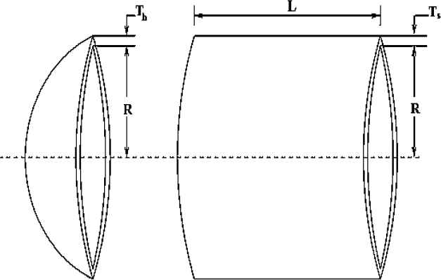
Schematic overview of pressure vessel design problem.
Magnitudes of loss functions over training sample points for two design variables in pressure vessel design problem.
Surface plots of Kriging surrogate fitted over training points and loss functions for two design variables in pressure vessel design problem.
(a) Feasible points regarding sorted grid points (search sample points) and (b) adaptive improvement for three optimal points obtained from sorted grid points in pressure vessel design problem.
3.4. Three-Bar Truss Design Problem
This structural optimization problem exists in the field of civil engineering. This problem is widely utilized as case studies in the literature because of its highly constrained search space [35,37]. As shown in Figure 16, two parameters need to be optimally defined to achieve the least weight subject to stress, deflection, and buckling constraints. This problem is mathematically formulated as follows:
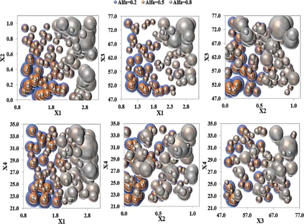
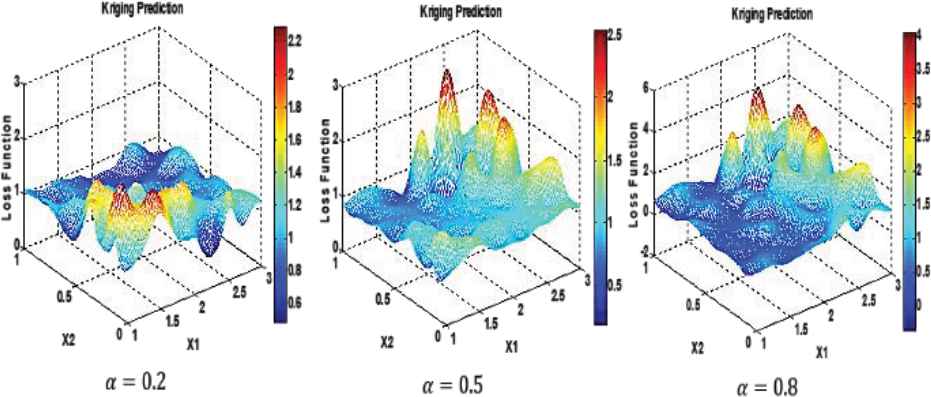
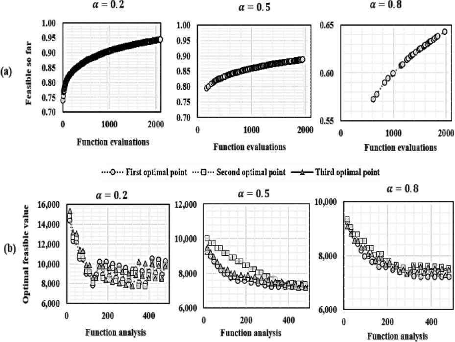
This problem with two dimensions was solved by the SGCO algorithm. The magnitudes of the overall loss function and 3D surface plots constructed by Kriging are shown in Figures 17 and 18, respectively. Figure 19(a) and 19(b) illustrate the feasible points obtained by the sorted grid points and the adaptive improvement for the three first best feasible points obtained by the sorted grid points. The results of the proposed algorithm are compared to some common evolutionary algorithms to solve the three-bar truss problem (with the same platform) such as hybridizing Particle Swarm Optimization with Differential Evolution (PSO-DE) [81], GOA [37], and ALO [12] are shown in Table 4. The results indicate that very competitive results are provided by SCGO in obtaining optimal results in the three-bar truss design problem. The optimal cost functions by SCGO are obtained in
| Algorithm | Optimum Variables |
Optimal Cost | Function Evaluations | ||||
|---|---|---|---|---|---|---|---|
| X1 | X2 | X3 | X4 | ||||
| SCGO | α = 0.2 | 1.26312 | 0.66255 | 64.50464 | 13.28434 | 7684.383 | 849 |
| α = 0.5 | 1.21502 | 0.59585 | 62.09559 | 24.28143 | 7157.687 | 1097 | |
| α = 0.8 | 1.21502 | 0.60394 | 62.09559 | 24.28143 | 7213.137 | 1452 | |
| GWO | 0.81250 | 0.43450 | 42.08918 | 176.75873 | 6051.564 | --- | |
| WOA | 0.81250 | 0.43750 | 42.09827 | 176.63900 | 6059.741 | 6300 | |
| GSA | 1.12500 | 0.62500 | 55.98866 | 84.45420 | 8538.836 | 7110 | |
| CPSO | 0.81250 | 0.43750 | 42.09127 | 176.74650 | 6061.078 | 14790 | |
SCGO, Surrogate-Based Constrained Global-Optimization; WOA, Whale Optimization Algorithm; GWO, Grey Wolf Optimizer; GSA, Gravitational Search Algorithm; SSA, Salp Swarm Algorithm; CPSO, Co-evolutionary Particle Swarm Optimization.
Comparison of SCGO optimization results with literature for the pressure vessel design problem.
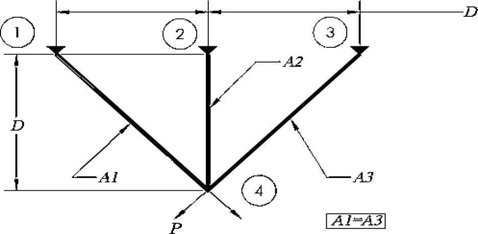
Schematic overview of three-bar truss design problem.
Magnitudes of loss functions over training sample points for two design variables in three-bar truss design problem.
Surface plots of Kriging surrogate fitted over training points and loss functions for two design variables in three-bar truss design problem.
(a) Feasible points regarding sorted grid points (search sample points) and (b) adaptive improvement for three optimal points obtained from sorted grid points in three-bar truss design problem.
4. DISCUSSION
4.1. Performance Measure
In many studies on optimization, the strength of an optimization technique is measured by comparing the final solution achieved by different algorithms [33,82]. This approach only provides information about the quality of the results and neglects the speed of convergence which is a very important measure for expensive optimization problems. Comparing the convergence curve (number of function evaluations) is also one of the common benchmarking approaches [59]. However, a convergence curve provides good information about the final quality of the optimization result in terms of computational cost and it can be used to compare the performance of several algorithms only in one problem. Moré and Wild [83] have suggested performance measure for any pair
| Algorithm | Optimum Variables |
Optimal Weight | Function Evaluations | ||
|---|---|---|---|---|---|
| X1 | X2 | ||||
| SCGO | α = 0.2 | 0.80889 | 0.35538 | 264.32708 | 222 |
| α = 0.5 | 0.74425 | 0.56917 | 267.42254 | 228 | |
| α = 0.8 | 0.76080 | 0.49944 | 265.12941 | 226 | |
| GOA | 0.78890 | 0.40762 | 263.89588 | 13000 | |
| ALO | 0.78866 | 0.40828 | 263.89584 | 14000 | |
| PSO-DE | 0.78868 | 0.40825 | 263.89584 | 17600 | |
SCGO, Surrogate-Based Constrained Global-Optimization; GOA, Grasshopper Optimization Algorithm; ALO, Ant Lion Optimizer; PSO-DE, Particle Swarm Optimization with Differential Evolution.
Comparison of SCGO optimization results with literature for the three-bar truss design problem.
However, Eq. (12) considers the required budget to solve the expensive optimization problem. In this study, inspired by [83], a new performance measure is used to consider two terms of the algorithm's performance including the level of accuracy and computational cost as follows:
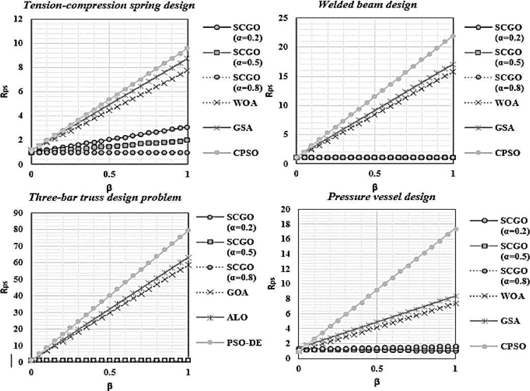
The performance comparison of Surrogate-Based Constrained Global-Optimization (SCGO) with other solvers in the literature for four common engineering design problems. The performance criterion
In addition to the desired performance of SCGO in obtaining an optimal solution with a very small number of function evaluations comparing to the commonly existing solvers, there are some other points regarding the SCGO algorithm as below:
Exploration: The SCGO algorithm employs space-filling design sampling methods (e.g. LHS) to construct Kriging surrogate. This method spreads sample points in the whole design space. However, the search procedure is performed in the whole design space using the grid-search method. The proposed algorithm searches for the optimal solution by employing Kriging instead of an expensive original model using the “grid- search” method. In this approach, the whole design space is studied through the evaluation model's components consisting of objectives and constraints set in the equally spaced grid points. In this searching method, there is a chance to find the global optimum solution because searching is not bounded to the local valley (global search).
Exploitation: In the proposed algorithm, the adaptive improvement is used to search in the region that the best feasible point is located (local search), see Algorithm 2.
The SCGO algorithm also provides very competitive results on the benchmark engineering design problems. This demonstrates that SCGO shows a good balance between exploration and exploitation to the avoidance of local optima.
4.2. Limitations of SCGO
There are some limitations of the proposed SCGO method as follows:
The SCGO method employs Kriging surrogate to train the overall loss function including integrated objective and constraint functions using space-filling sampling strategies. Therefore, the approximate errors cannot be ignored when solving inequality-constrained simulation-optimization problems particularly with complex function and nonlinear structure. It is well known that Kriging models are ideal candidates for smooth models. If the functions are nonsmooth or noisy, it is likely that Kriging surrogate degrades rapidly and overfit due to their interpolating behavior. A challenge for optimization under restricted budgets will be to find the right degree of approximation (smoothing factor) from only relatively few samples [33].
This study aims to provide a fair comparison between the proposed algorithm and the highly referred methods in the literature [10–12,84,85] for solving benchmark problems. Therefore, the same framework has been taken from the mentioned studies (i.e., the problems with all inequality constraints). In [85] and [33], a reformulation of an equality constraint of
This study aims to provide a fair comparison between SCGO and the highly referred methods in the literature for solving problems in practical engineering design optimization. Therefore, the same framework (low-dimensional optimization problems) have been taken from studies [10–12,84,85]. However, in this study, the application of SCGO is limited to low-dimensional optimization problems.
5. CONCLUSION
In the paper, the SCGO algorithm is developed to solve simulation-based optimization problems with a computationally expensive objective and constraints. Kriging surrogate is used to approximate the computational expensive overall loss function. Firstly, an overall loss function is constructed to integrate objective and constraint functions in the same overall objective function. Secondly, the Kriging surrogate is constructed using a small number of simulation experiments. Then, the adaptive improvement approach is performed to further improve the optimal solution while enforcing a feasible solution. The grid-search strategy is used to effectively perform exploration in whole design space and the avoidance of local optima. The proposed algorithm is tested using several constrained global optimization problems. The results indicate that the SCGO method is effective for solving expensive constrained optimization problems with a much smaller number of function evaluations comparing to some state-of-the-art metaheuristics.
Future research will be devoted to overcoming the current limitations of SCGO mentioned in Section 4.2. It would be interesting to extend the proposed SGCO algorithm to handle high-dimensional-constrained optimization problems while keeping performance in obtaining optimal solutions with a small number of function evaluations. Besides, the SGCO algorithm can be extended to cover equality constraints as well as inequality constraint functions. Kriging can be replaced with other interpolation methods such as radial basis function, support vector machine, or artificial neural network. Besides, the application of SCGO can be developed to handle a higher dimension of optimization problems in the practice of constrained engineering design problems.
CONFLICTS OF INTEREST
The authors declare that they have no conflicts of interests.
AUTHORS' CONTRIBUTIONS
All authors have contributed equally to this study. All authors read and approved the final manuscript.
ACKNOWLEDGMENTS
This research project is supported by Second Century Fund (C2F), Chulalongkorn University, Bangkok, Thailand.
REFERENCES
Cite this article
TY  - JOUR
AU  - Amir Parnianifard
AU  - Ratchatin Chancharoen
AU  - Gridsada Phanomchoeng
AU  - Lunchakorn Wuttisittikulkij
PY  - 2020
DA  - 2020/10/23
TI  - A New Approach for Low-Dimensional Constrained Engineering Design Optimization Using Design and Analysis of Simulation Experiments
JO  - International Journal of Computational Intelligence Systems
SP  - 1663
EP  - 1678
VL  - 13
IS  - 1
SN  - 1875-6883
UR  - https://doi.org/10.2991/ijcis.d.201014.001
DO  - 10.2991/ijcis.d.201014.001
ID  - Parnianifard2020
ER  -