
An Adaptive Multi-Objective Evolutionary Algorithm with Two-Stage Local Search for Flexible Job-Shop Scheduling
 , Zhengwei Liu
- DOI
- 10.2991/ijcis.d.201104.001How to use a DOI?
- Keywords
- Flexible job-shop scheduling; Multi-objective optimization; Evolutionary algorithm; Local search
- Abstract
An adaptive evolutionary algorithm with two-stage local search is proposed to solve the multi-objective flexible job-shop scheduling problem (MOFJSP). Adaptivity and efficient solving ability are the two main features. An autonomous selection mechanism of crossover operator is designed, which divides individuals into different levels and selects the appropriate one according to the both sides' levels to improve the self-adaptation. In parameter setting, the autonomous determination and adjustment mechanism is proposed, and parameters are adjusted autonomously according to the job scale and iteration number, so as to reduce the complexity of parameter setting and further improve the adaptivity. For improving solving ability, two-stage local search mechanism is designed. The first stage is performed before the evolution operation, so that each individual has more good genes to participate in the following operation. The second stage is performed after the evolution operation to further search the optimal solutions. Finally, a large number of comparative numerical tests are carried out, compared with other excellent algorithms, the proposed algorithm has fewer parameters to be set and stronger solving ability.
- Copyright
- © 2021 The Authors. Published by Atlantis Press B.V.
- Open Access
- This is an open access article distributed under the CC BY-NC 4.0 license (http://creativecommons.org/licenses/by-nc/4.0/).
1. INTRODUCTION
Job-shop scheduling problem (JSP) is a branch of production scheduling and one of the most arduous combinatorial optimization problems [1]. In the classical JSP, a set of
Flexible job-shop scheduling problem (FJSP) is an extension of the classical JSP. Unlike JSP issue, FJSP breaks the restriction of unique resources, operations are allowed to be processed on any among a set of available machines. Therefore, compared with JSP, FJSP is closer to the actual production situation. Because of the additional need to determine the assignment of operations on the machines, FJSP is more complex than JSP, and incorporates all the difficulty and complexity of JSP [4].
Brucker and Schlie [5] were the first to address the FJSP. They proposed a polynomial algorithm for solving the FJSP with two jobs, in which the machines capable of performing one operation have the same processing time. Commonly there are two methods for solving FJSP: hierarchical approach and integrated approach. Hierarchical approach was first proposed by Brandimarte [6]. Its basic idea is decomposing the complex problem into some sub-problems in order to decrease the complexity, i.e., it considered the assigning sub-problem and the sequencing sub-problem separately. However, in integrated approach, the assigning sub-problem and the sequencing sub-problem are solved simultaneously.
There have been many single-objective studies on FJSP, but the multi-objective flexible job-shop scheduling problem (MOFJSP) is more in line with the need of actual production. MOFJSP has been studied by many researchers in past decades. Xia and Wu [7] proposed a hierarchical solution approach by using a particle swarm optimization algorithm to assign operations on machines and a simulated annealing algorithm to schedule operations on each machine. Zhang et al. [8] proposed an effective hybrid approach for the MOFJSP, hybridizing the two optimization algorithms, particle swarm optimization and tabu search algorithm. Baykasoǧlu et al. [9] presented a linguistic-based meta-heuristic modeling and multi-objective tabu search algorithm to solve the MOFJSP. Ho and Tay [10] studied a hybrid evolution algorithm combined with a guided local search and external Pareto archive set (AS).
Evolutionary algorithm (EA) is an intelligent optimization algorithm inspired by biology, which has been widely used in solving MOFJSP. The existing algorithms have poor self-adaptability. Specifically, the evolutionary operation does not consider the differences of individuals, and cannot make dynamic adjustment according to the individuals' differences. Also, the parameter setting process is complex and lacks flexibility. When the test case is replaced, parameters need to be reoptimized. In addition, how to improve the algorithm's solution performance is also a current bottleneck. To solve the above problems, the EA is improved in many aspects in this paper, as shown in Figure 1.
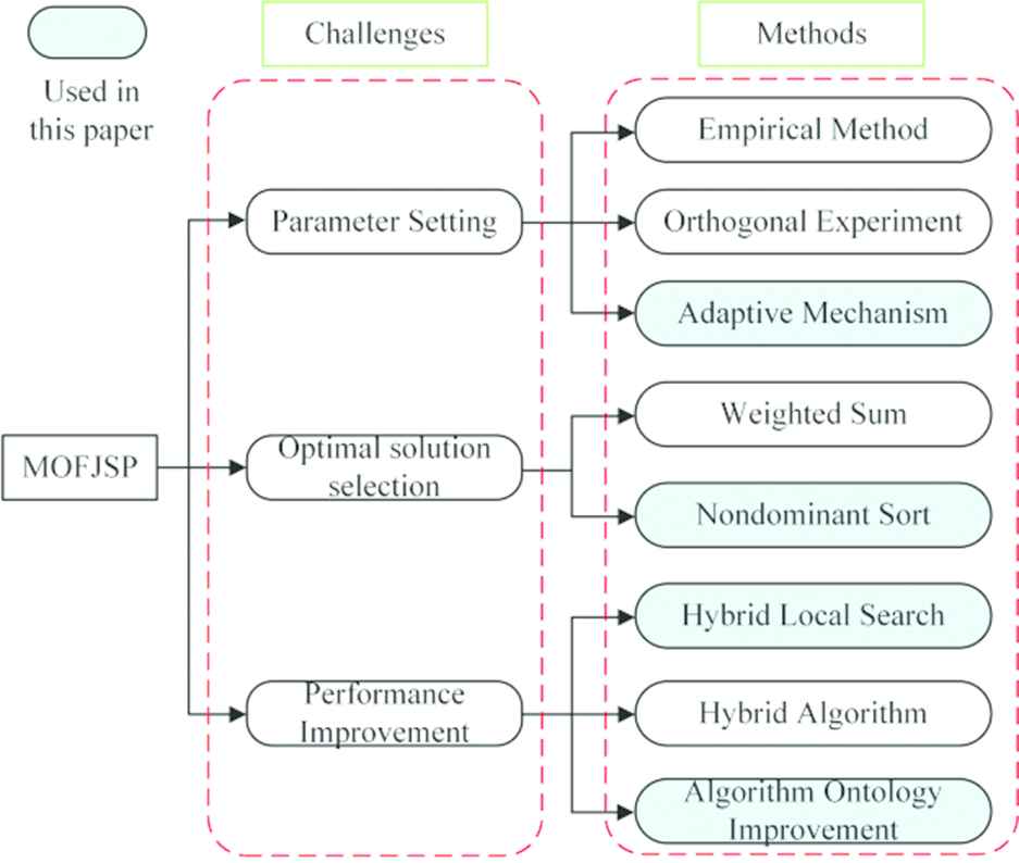
Challenges and overcome methods.
In this paper, an adaptive evolutionary algorithm with two-stage local search is proposed. First, the individual coding scheme was improved. To adapt to the scheme, new methods of individual crossover, mutation and selection were designed. In terms of crossover operation, considering the differences between individuals, different crossover operators are designed. Individuals of different levels can select the appropriate crossover operator, thereby improving the algorithm's adaptive ability and solving ability. Second, an adaptive parameter adjustment mechanism is designed to further improve the adaptive ability. The algorithm can autonomously adjust the parameters according to the scale of the jobs and the number of iterations, thus reducing the complexity of parameter setting. Finally, a two-stage local search is embedded in the algorithm. The first stage is before the evolution operation to allow individuals to have more good genes, and the second stage is after the evolution operation to search for more superior solutions, consequently further improve the solving ability of the algorithm.
The remainder of the paper is organized as follows: In Section 2, the assumptions and formulations of MOFJSP are described in detail. In Section 3, the scheme of the proposed algorithm for MOFJSP is elaborated. In Section 4, the computational results and the comparison with other approaches are presented. The final conclusions are given in Section 5.
2. PROBLEM FORMULATION
2.1. MOFJSP Description
The MOFJSP is described as follows [11]: there are
One machine can only process one job at a time, and one job can only be processed only on one machine at a time.
There is a priority restriction between every two different operations of the same job, i.e., only after the previous operation is completed, the next one can be processed.
The operations of different jobs do not have precedence constraints.
All jobs have equal priorities, all machines are independent and each machine is ready at zero time.
Once one operation is started, it will not be interrupted until the process is finished.
Moving time between operations and setting up time of machines are negligible.
The notation used in this paper is summarized in the follows:
| - |
Index of jobs |
| - |
Index of operations |
| - |
Index of machines |
| - |
Total number of jobs |
| - |
Total number of machines |
| - |
Total number of operations of job |
| - |
The |
| - |
The |
| - |
The set of available machines for the operation |
| - |
Makespan (the maximal completion time) |
| - |
Critical machine workload (the machine with the biggest workload) |
| - |
Total workload of machines (the total working time of all machines) |
| - |
Processing time of |
| - |
Processing time of |
| - |
Decision variable |
| - |
Decision variable |
| - |
Completion time of job |
| - |
Completion time of operation |
| - |
Completion time of operation |
In this paper, three objectives will be optimized simultaneously, as follows [12]:
Subject to:
2.2. Basic Concepts of Multi-Objective Optimization
Multi-objective optimization problem is usually defined in the following form [14]:
Existing research approaches for multi-objective optimization problem can be categorized into three: Pareto dominance-based, aggregation-based and lexicographical order-based, and most of the research are on the first two. Due to the superiority of the Pareto dominance-based approach in the number of solutions, and no need to consider the weight assignment problem among multiple sub-objectives, this paper chooses Pareto dominance-based approach to solve the multi-objective optimization problem.
The goal of Pareto dominance-based approach is to obtain all the nondominated solutions, which are referred to as Pareto-optimal solutions. The definition of Pareto dominance and Pareto optimality are given as follows:
Nondominated solutions
Solution
Pareto optimality
A solution
3. THE PROPOSED EA
3.1. Encoding and Decoding Scheme
The proposed algorithm optimizes assigning sub-problem and sequencing sub-problem simultaneously, and thus the information of operations and related machines should be encoded in the same chromosome. Two encoding schemes are commonly used to solve MOFJSP [15]: A-B string [8,16,17] and 3-tuple scheme [18–20]. Both schemes represent the same information, and the difference is only in the implementation. In 3-tuple scheme, a gene includes three elements which are the job number, the operation number and the assigned machine. However, in A-B string, two genes are needed to represent the same information. So, 3-tuple scheme is simpler and more intuitive than A-B string in the manner of representation, and the chromosome length of 3-tuple is only half of A-B strings. In this paper, a new encoding scheme, called 2-tuple, is designed for MOFJSP, which is improved on the basis of 3-tuple, and it is more concise than 3-tuple because a gene goes from three elements to two.
Each chromosome is a sequence of genes. A gene is a 2-tuple
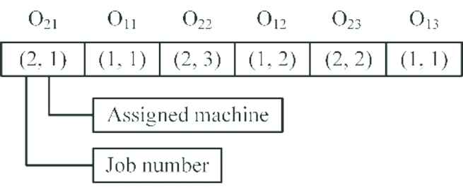
Chromosome encoding.
Decoding is the process of converting each chromosome to scheduling solution. Schedules are grouped into three types by [21]: non-delay schedule, semi-schedule and active schedule. It has been proved that active schedule contains the optimal schedule. In an active schedule, no operation can be processed in advance except putting off another operation's start time or changing the order of operations [22]. In order to obtain active schedule, this paper introduces the left-shift greedy decoding scheme [23]. The advantage of this scheme is that it has a self-repairing mechanism, always searching a sufficient and suitable idle time interval for each operation on the processing machine without delaying any other operations, so as to shift the operation to the left as compact as possible. The detailed procedures are shown as follows:
Step 1: Read gene sequence of a chromosome from left to right successively. Assuming a gene
Step 2: Search the first idle time interval
Step 3: Identify the beginning time of operation
Step 4: Evaluate the condition of left-shift. If there is enough time from
Step 5: Update chromosome. Due to the employ of the left-shift greedy decoding scheme, operation
3.2. Population Initialization
The quality of initial population is very important for accelerating convergence speed and avoiding premature convergence. It has been proved that utilizing a hybrid multi-approach to generate initial population is better than using single one in the performance [20]. Thus, in this paper, an approach of integrating strategies is employed for generating initial population. It includes five assignment rules and four sequencing rules.
Assignment rules
Random rule: It assigns each operation to a capable machine randomly.
Minimum processing time rule [20]: For every operation, the machine with the minimum processing time will be selected in the corresponding operation's candidate machine set. If there are multi-machines with the same minimum processing time, select one from them randomly, then assign the operation to the selected machine.
Global minimum processing time rule [20]: From the processing time table, find the minimum processing time among all operations, fix the assignment, then add the selected processing time to every other entry in the same column, and conduct the next time selecting, until all operations are assigned. If there are multi-global minimum processing time, select one randomly.
Local minimum processing time rule [23]: Find the minimum processing time from the first operation of the first job to the last operation of the last job successively. For each operation, the selected time will be added to other entry in the same column for conducting next time selecting, and each operation will be assigned to the corresponding selected machine. If there are multi-local minimum processing time, select one randomly.
Permutation rule: Shuffle the order of operations in processing time table randomly. Take the operation in the first row as the starting operation to select the machine with minimum processing time, fix the assignment, then add the selected processing time to every other entry in the same column for conducting next time's selecting. If there are multi-machines have the same minimum processing time, randomly select one.
Sequencing rules
Random rule: It places the operations into a chromosome in a random order.
Most work remaining rule [6]: One operation is selected according to the remaining work time of all jobs and be placed into a chromosome. The larger the remaining work time is, the earlier the operation of corresponding job can be selected. If there are multi-jobs have the same remaining work time, select one randomly.
Most number of operations remaining rule [20]: This rule select operation according to the remaining number of operations, the more the remaining number of operations is, the earlier the operation of corresponding job can be selected. If there are multi-jobs have the same remaining number of operations, select one randomly.
Shortest processing time rule [6]: The first operations of the remaining operations from each job are compared, the operation with the minimum processing time will be selected preferentially.
In the researches that utilizing hybrid multi-strategies to generate initial population, commonly a percentage-based approach, allocating different percentages for each approach to generate the required initial population, is adopted. In this paper, a new loop-based method is designed to generate initial population, and the difference is percentage allocation is not needed for each strategy compared with some other excellent algorithm, e.g., EPABC proposed in [13], AIA proposed in [18], etc. The utilization of loop-based method helps to increase the diversity of population and to extend the search space. The detailed procedure is described as follows:
Step 1: Place 20
Step 2: A combination is successively selected in the manner of loop from
Step 3: Repeat perform step 2 until the number of initial individuals reaching
3.3. Local Search I (LS-I)
Local search is an effective method to exploit better solution around a current solution. It has been widely used in MOFJSP. Inspired by the idea of left-shift greedy decoding scheme (mentioned in Section 3.1), also for keeping initial population's distribution characteristics, a new local search method is proposed. The performing process of LS-I is described as follows:
Step 1: Take out one chromosome from population, decode the chromosome, obtain three objective's value
Step 2: Decode again. Due to different operations of the same job have precedence constrains and parent population commonly is not the optimal solutions, there are some idle time interval existing in a scheduling solution. Read a gene
Step 3: Judgment. If the moving of operation
Step 4: Repeat step 2 to step 3, until all genes on the chromosome are decoded. Repeat step 1 to step 3, until all the individuals in initial population are optimized.
In order to better illustrate LS-I, taking Figure 3 as a simple example, moving operation
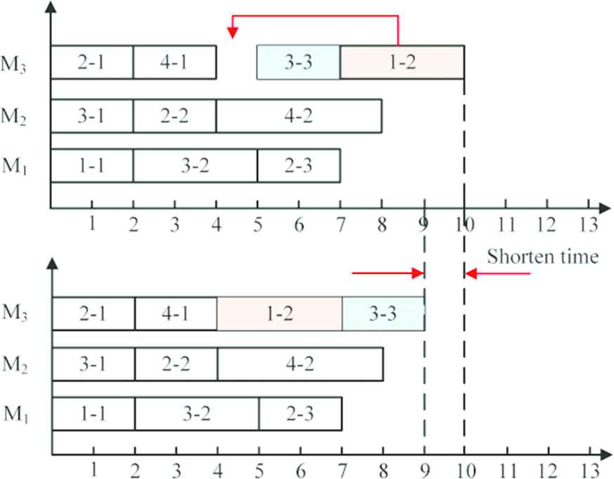
Local search before evolution operation.
3.4. Crossover Operators
The goal of crossover is to obtain two offsprings which inherit the gene information from their parent's chromosomes and generate new superior gene sequences. In this algorithm, crossover includes two parts: crossover for operation sequence and crossover for machine assignment. These two parts are implemented separately, and the terminal condition is that the amount of offspring equals
Crossover for operation sequence
Many effective approaches are developed for operation sequence's crossover in the past decades, such as order crossover employed by [16], HCO proposed by [12], IPOX designed by [11]. In this paper, considering the chromosome structure, IPOX is adopted. In addition, a new crossover approach, called RPOX, is proposed on the basis of IPOX, so the proposed algorithm can adaptively select one from the two crossover approaches according to the quality of the parent's chromosomes to generate good offspring. The details of IPOX and RPOX are shown as follows:
Step 1: Fast nondominated sorting [24] is performed for initial population which is divided into different ranks
Step 2: Randomly select two individuals
Step 3: Copy the elements of
Step 4: If the elements of
Step 5: If the parent's chromosomes are in the inferior population, RPOX is adopted. Otherwise, IPOX is adopted. Because the chromosomes selected from the inferior population always possess few good gene information, only with the large change, the offspring can possibly generate useful gene sequence. On the contrary, the chromosomes selected from the excellent population possess good gene sequence, so small change should be made to keep the good gene information to the next generation.
Crossover machine assignment
After operation sequence's crossover is completed, crossover for machine assignment should be performed to determine the machine for each operation in children's chromosomes
Step 1: Two integers
Step 2: The genes of
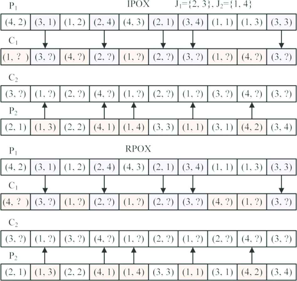
IPOX and RPOX crossover operation for the operation sequence.
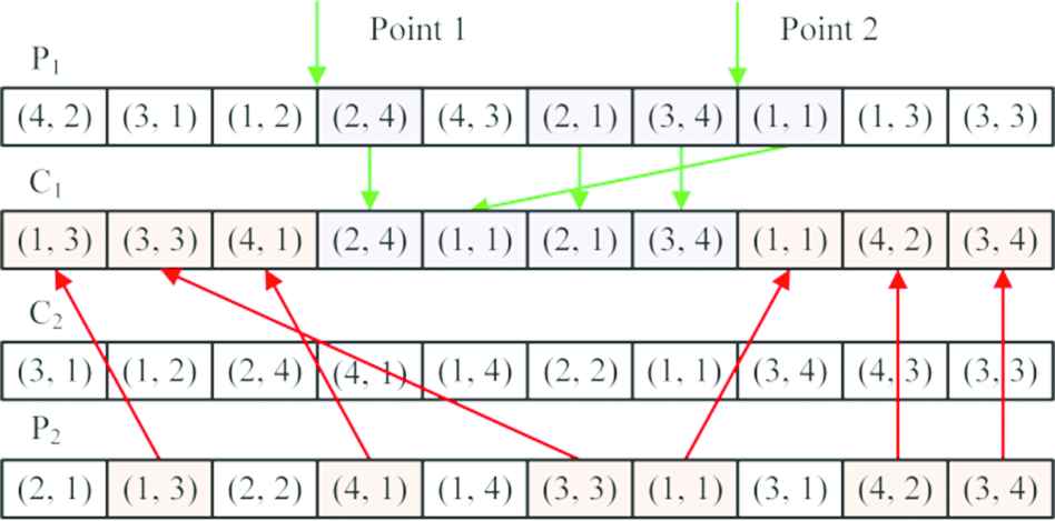
ITP crossover operation for the machine assignment.
3.5. Mutation Operators
Mutation is one of the key technologies for avoiding premature and increasing the diversity of population. A substitution method is adopted in this paper. For operation sequence's mutation, two genes that do not belong to the same job are selected randomly, then their position will be swapped and the corresponding machine information will be updated.
For machine assignment's mutation, the machine
3.6. Environment Selection
Environment selection is to select certain amounts of individuals, called new initial population or survived individuals, from the population of parent and children. The survived individuals will be participated in the next time's genetic operation. For environment selection, fitness-based [7] and dominance-based [25] selection methods have been developed and widely used in scheduling problem. Due to the advantage of dominance-based method in term of considering the tradeoff among multi-objectives, it is adopted in this paper.
In dominance-based method, crowding distance [25] is commonly used to select certain individuals from the subpopulation with the same rank. It is effective to the optimization problem with two objectives, but with three objectives it is insufficient to some extent. In order to keep the diversity of the new initial population, a partition selection method is designed to replace crowding distance. The details of environment selection are described as follows:
Step 1: Fast nondominated sorting is performed for all individuals and divided them into different levels
Step 2: If
Step 3: All individuals in
Step 4: An external AS is imbedded in the proposed algorithm. The individuals in
3.7. Local Search II (LS-II)
The purpose of LS-I mentioned in Section 3.3 is to make the chromosome carry more superior genes in a short time. However, a new local search method, called LS-II, based on the critical path is purposed to find more promising solutions. The emphasis of the two methods are different, LS-I pursues speed, LS-II pursues quality.
In this paper, a concept, called full sequence, is proposed. If no time interval exists between every two adjacent operations on the same machine, this state is called a full sequence, e.g.,
In order to optimize three objectives simultaneous, the local search method based on critical path is extended. It includes two parts: reassignment and shifting critical operations. Compared with some methods that only shifting critical operations, LS-II not only reduce the makespan (
Step 1: According to the result of fast nondominated sorting in Section 3.6, the individuals in
Step 2: Take out a chromosome
Step 3: Shifting critical operation. First, identify the critical paths and the critical blocks on the chromosome. Let
Step 4: Reassignment. In all full sequences, if an operation has at least one candidate machine and the candidate machine's processing time is not larger than the current one, this operation is called reassignment operation and these candidate machines compose the replacement machine subset. Select one reassignment operation randomly, select the machine that has the minimum workload from the replacement machine subset, and move the selected operation to the selected machine. If some machines have the same minimum total workload, select one randomly. Repeat performing reassignment until the number of performing equals to the total sum of reassignment operations. If the new chromosome is better than the old one, the chromosome will be recorded. The best one in all new chromosomes will replace the old chromosome. This step can realize reducing the makespan (
Step 5: Repeat step 1 to step 4, until all the individuals in
3.8. Main Algorithm
The framework of the proposed algorithm for MOFJSP can be shown in Figure 6.
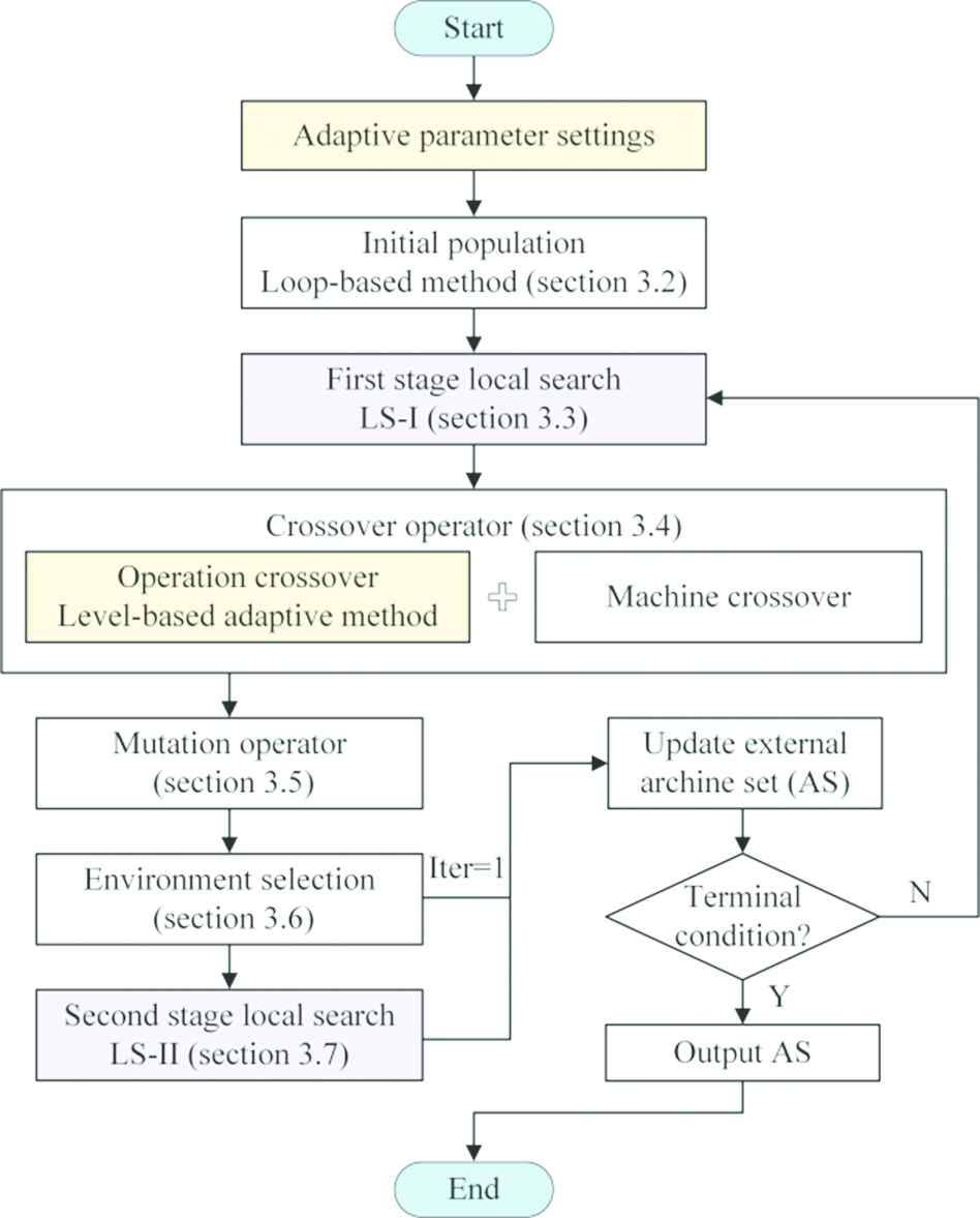
The flowchart of the proposed algorithm.
Step 1: Initialization. Loop-based method (Section 3.2) is used to generate initial population
Step 2: Apply LS-I (Section 3.3) to optimize all individuals in
Step 3: Perform crossover operators (Section 3.4) and mutation operators (Section 3.5) to generate offspring populations
Step 4: Merge
Step 5: Apply LS-II (Section 3.7) to search more promising solutions, update
Step 6: If the terminating condition is satisfied, the algorithm ends. else, go to step 2.
4. EXPERIMENTAL RESULTS
4.1. Parameter Setup
The process of determining the feasible parameter is complex in some researches. To simplify the process, in our algorithm, very few parameters are needed, and an adaptive parameter setup method is designed. The amount of initial population
4.2. Result and Comparison
To test the performance of the proposed algorithm, the algorithm procedure was implemented in python and run through the PyCharm software on a PC with AMD A-8 6410 2.0 GHz CPU 4.0 G RAM and Windows 10 operating system. Four representative instance sets based on the practical data have been selected. The first one is taken from [26], which includes 10 small size problem instances (SFJS01:10) and 10 medium and large size problem instances (MFJS01:10). The second one is taken from [27] without release time, which includes five problem instances (problem
The algorithm's advantage is that very few parameters setup is needed. Table 1 gives a comparison of several state-of-the-art algorithm's number of parameters, including Li et al. [17,29], Wang et al. [11] and Xing et al. [30]. From this table, the number of parameters needed in the proposed algoithom is the least, which is three.
| Author | Framework | Fitness Assignment | Number of Parameters |
|---|---|---|---|
| Li and Pan | ABC | Dominance | 4 |
| Li | TS | Weighted sum | 6 |
| Wang | GA | Dominance | 4 |
| LS | Weighted sum | 13 | |
| Proposed | GA + LS | Dominance | 3 |
Compare in the number of parameters.
In order to test the effect of improved coding, crossover, mutation, population generation and environment selection methods on the performance of the proposed algorithm, the two-stage local search was removed from the proposed algorithm, and the remaining part (IEEA) was tested together with the traditional EA through the same case. The proposed algorithm is called IEA. The test case set uses SFJS01-10 and MFJS01-10. The EA is selected from the literature [15], which uses a variety of combination strategies, and has proved to be more superior than other classic EAs. In this section, metric
| Item | EA and IEEA |
IEEA and IEA |
||
|---|---|---|---|---|
| C (EA, IEEA) | C (IEEA, EA) | C (IEEA, IEA) | C (IEA, IEEA) | |
| SFJS01 | 0.00 | 1.00 | 0.00 | 0.00 |
| SFJS02 | 0.00 | 1.00 | 0.00 | 0.00 |
| SFJS03 | 0.00 | 1.00 | 0.00 | 0.00 |
| SFJS04 | 0.00 | 1.00 | 0.00 | 0.00 |
| SFJS05 | 0.00 | 1.00 | 0.00 | 0.00 |
| SFJS06 | 0.00 | 1.00 | 0.00 | 0.00 |
| SFJS07 | 0.00 | 1.00 | 0.00 | 0.00 |
| SFJS08 | 0.00 | 1.00 | 0.00 | 0.00 |
| SFJS09 | 0.00 | 0.78 | 0.00 | 0.22 |
| SFJS10 | 0.00 | 1.00 | 0.00 | 0.40 |
| MFJS01 | 0.00 | 0.88 | 0.00 | 0.14 |
| MFJS02 | 0.07 | 0.44 | 0.00 | 0.79 |
| MFJS03 | 0.50 | 0.10 | 0.00 | 0.86 |
| MFJS04 | 0.00 | 0.24 | 0.00 | 0.22 |
| MFJS05 | 0.00 | 0.73 | 0.00 | 0.63 |
| MFJS06 | 0.00 | 0.94 | 0.00 | 0.33 |
| MFJS07 | 0.68 | 0.08 | 0.14 | 0.53 |
| MFJS08 | 0.00 | 1.00 | 0.00 | 0.00 |
| MFJS09 | 0.00 | 1.00 | 0.00 | 0.30 |
| MFJS10 | 0.00 | 1.00 | 0.00 | 0.81 |
The test result of SFJS01-10 and MFJS01-10.
It can be seen from Table 2 that in the 20 problem instances, IEEA is superior to EA except MFJS03 and MFJS07. Compared with IEEA, IEA does not show obvious advantage in 10 small size problem instances, indicating that for small size problem instances IEA can find the optimal solution without local search, while for 10 medium and large size problem instances, IEA has shown obvious advantage. In addition, the frontier of EA, IEEA and IEA on MFJS02, MFJS03, MFJS05 and MFJS10 are given, as shown in Figure 7. It can also be seen from the figure that IEEA is better than EA, and IEA is better than IEEA.
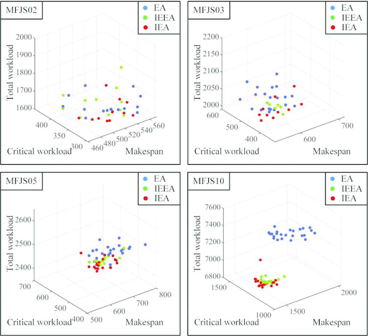
The frontier of EA, IEEA and IEA on problem instances MFJS02, MFJS03, MFJS05 and MFJS10.
In order to test the overall performance of the proposed algorithm, it was tested on other three instance sets with several state-of-the-art algorithms.
For five problem instances, four state-of-the-art algorithms in Table 1 are also used to compare with the proposed algorithm. The reason of doing this is that the four algorithms are powerful, and it has been proved that it is better than other well-known algorithms (e.g., PSO+SA proposed by [7], AL+CGA proposed by [31], etc.). Hence, if the proposed algorithm is better than the four powerful algorithms, it is also better than PSO+SA and AL+CGA, etc.
Before comparison, some terms should be clarified. Optimal solutions in this paper refer to the nondominated solutions obtained by each algorithm. Pareto front is constructed by the optimal solutions of all compared algorithms and Pareto solutions refer to the solutions in Pareto front. All solutions in the Pareto front are called overall Pareto solutions. If some optimal solutions in a compared algorithm's optimal solutions are the Pareto solutions simultaneously, they are called partial Pareto solutions.
First, compare the amount of optimal solutions. Table 3 is the result of optimal solutions' amount. From this table, the proposed algorithm can obtain the best results for all problem instances. In problem
| Size | Method | Li and Pan |
Li |
Wang |
Xing |
Proposed |
|||||||||||||
|---|---|---|---|---|---|---|---|---|---|---|---|---|---|---|---|---|---|---|---|
| Objects | 1 | 2 | 3 | 1 | 2 | 3 | 1 | 2 | 3 | 4 | 1 | 2 | 3 | 4 | 1 | 2 | 3 | 4 | |
| f1 | 11 | 12 | 13 | 11 | 12 | – | 11 | 11 | 12 | – | 11 | 11 | 12 | – | 11 | 11 | 12 | 13 | |
| f2 | 10 | 8 | 7 | 10 | 8 | – | 10 | 9 | 8 | – | 10 | 9 | 8 | – | 10 | 9 | 8 | 7 | |
| f3 | 32 | 32 | 33 | 32 | 32 | – | 32 | 34 | 32 | – | 32 | 34 | 32 | – | 32 | 34 | 32 | 33 | |
| f1 | 14 | 15 | 16 | 14 | 15 | – | 15 | 15 | 16 | – | 14 | 15 | 16 | 17 | 14 | 15 | 16 | 16 | |
| f2 | 12 | 12 | 13 | 12 | 12 | – | 11 | 12 | 13 | – | 12 | 12 | 11 | 13 | 12 | 12 | 11 | 13 | |
| f3 | 77 | 75 | 73 | 77 | 75 | – | 81 | 75 | 73 | – | 77 | 75 | 77 | 73 | 77 | 75 | 77 | 73 | |
| f1 | 12 | 11 | 12 | 11 | 11 | – | – | – | – | – | 11 | 11 | 12 | – | 11 | 11 | 12 | – | |
| f2 | 11 | 11 | 12 | 11 | 10 | – | – | – | – | – | 11 | 10 | 12 | – | 10 | 11 | 12 | – | |
| f3 | 61 | 63 | 60 | 61 | 62 | – | – | – | – | – | 61 | 62 | 60 | – | 62 | 61 | 60 | – | |
| f1 | 8 | 7 | 8 | 7 | 7 | 8 | 8 | 7 | 8 | 7 | 7 | 8 | 8 | – | 7 | 7 | 8 | 8 | |
| f2 | 7 | 5 | 5 | 5 | 6 | 5 | 5 | 6 | 7 | 5 | 6 | 7 | 5 | – | 6 | 5 | 7 | 5 | |
| f3 | 41 | 43 | 42 | 43 | 42 | 42 | 42 | 42 | 41 | 45 | 42 | 41 | 42 | – | 42 | 43 | 41 | 42 | |
| f1 | 12 | 11 | – | 11 | 11 | – | 11 | 12 | 11 | – | 11 | – | – | – | 11 | 11 | – | – | |
| f2 | 11 | 11 | – | 11 | 10 | – | 11 | 10 | 10 | – | 11 | – | – | – | 11 | 10 | – | – | |
| f3 | 91 | 93 | – | 91 | 93 | – | 91 | 95 | 98 | – | 91 | – | – | – | 91 | 93 | – | – | |
The optimal solutions of each algorithm for five problem instances.
Second, compare the quality of optimal solutions. Table 4 gives an overall perspective of optimal solutions' quality. In this table,
| Size | H | Li and Pan |
Li |
Wang |
Xing |
Proposed |
||||||||||
|---|---|---|---|---|---|---|---|---|---|---|---|---|---|---|---|---|
| N/M | Q | R | N/M | Q | R | N/M | Q | R | N/M | Q | R | N/M | Q | R | ||
| 4 | 3/3 | 100 | 75 | 2/2 | 100 | 50 | 3/3 | 100 | 75 | 3/3 | 100 | 75 | 4/4 | 100 | 100 | |
| 5 | 3/3 | 100 | 75 | 2/2 | 100 | 40 | 3/3 | 100 | 60 | 4/3 | 75 | 60 | 4/4 | 100 | 80 | |
| 3 | 3/1 | 33.3 | 33.3 | 2/2 | 100 | 66.7 | – | – | – | 3/3 | 100 | 100 | 3/3 | 100 | 100 | |
| 4 | 3/3 | 100 | 75 | 3/3 | 100 | 75 | 4/3 | 75 | 75 | 3/3 | 100 | 75 | 4/4 | 100 | 100 | |
| 2 | 2/0 | 0 | 0 | 2/2 | 100 | 100 | 3/1 | 33.3 | 50 | 1/1 | 100 | 50 | 2/2 | 100 | 100 | |
| Sum | 18 | 14/10 | 71.4 | 55.6 | 11/11 | 100 | 61.1 | 13/10 | 76.9 | 55.6 | 14/13 | 92.9 | 72.2 | 17/17 | 100 | 94.4 |
The quality of optimal solutions I.
From Table 4, all the optimal solutions obtained by the proposed algorithm in the five problem instances are Pareto solutions, and, in each problem instance except problem
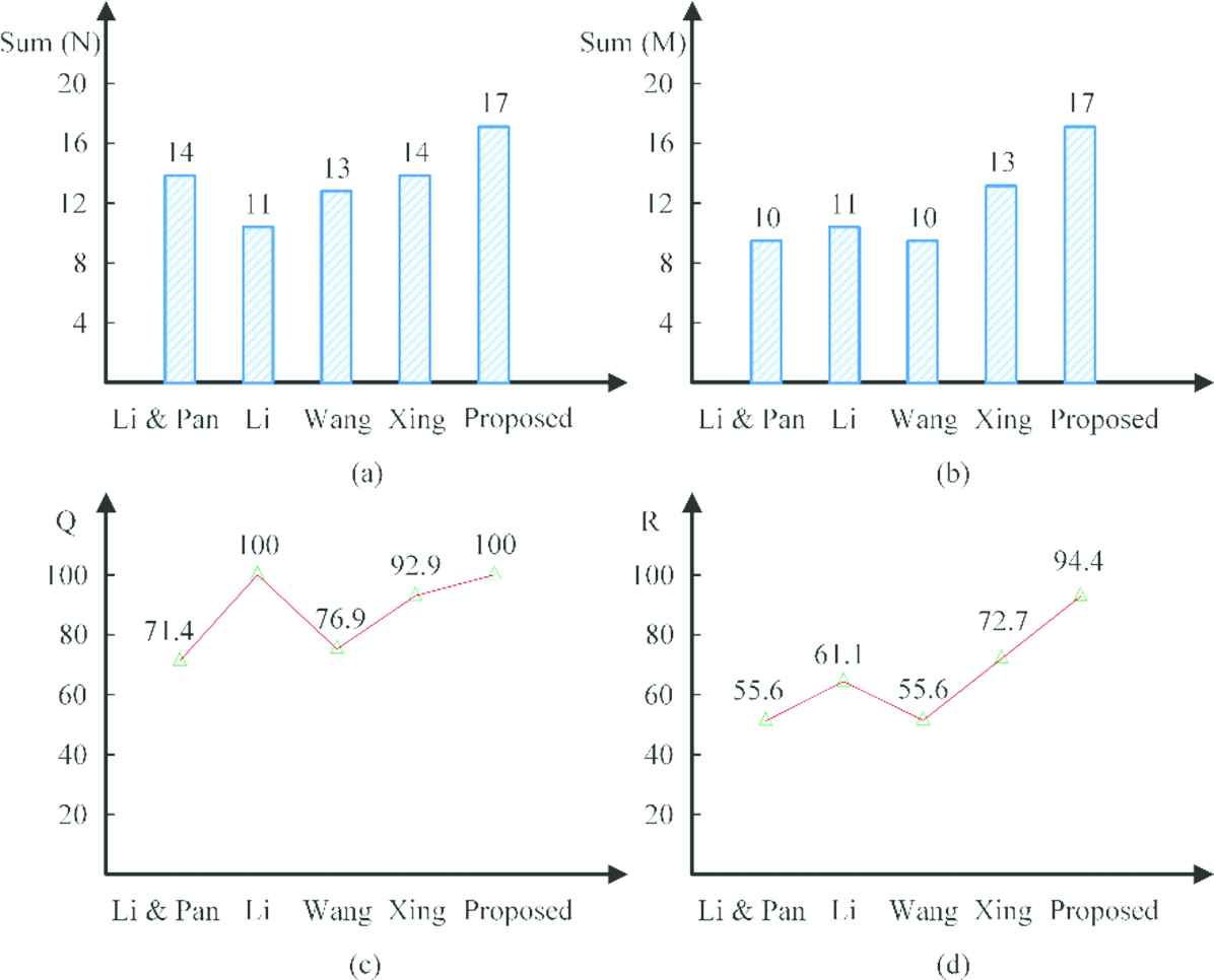
Statistic result on N, M, Q and R.
Table 5 gives a result from a local perspective, i.e., taking every one in the four state-of-the-art algorithms to compare with our algorithm. In this table, metric
| Size | Li and Pan (A1) |
Li (A2) |
Wang (A3) |
Xing (A4) |
||||
|---|---|---|---|---|---|---|---|---|
| C (A1, B) | C (B, A1) | C (A2, B) | C (B, A2) | C (A3, B) | C (B, A3) | C (A4, B) | C (B, A4) | |
| 0.000000 | 0.000000 | 0.000000 | 0.000000 | 0.000000 | 0.000000 | 0.000000 | 0.000000 | |
| 0.000000 | 0.000000 | 0.000000 | 0.000000 | 0.000000 | 0.000000 | 0.000000 | 0.250000 | |
| 0.000000 | 0.666667 | 0.000000 | 0.000000 | – | – | 0.000000 | 0.000000 | |
| 0.000000 | 0.000000 | 0.000000 | 0.000000 | 0.000000 | 0.250000 | 0.000000 | 0.000000 | |
| 0.000000 | 1.000000 | 0.000000 | 0.000000 | 0.000000 | 0.666667 | 0.000000 | 0.000000 | |
The quality of optimal solutions II.
From this table, all optimal solutions obtained by the proposed algorithm are not dominated by any optimal solution obtained by other compared algorithms in the five problem instances. However, at least one optimal solution obtained by the proposed algorithm can dominate some optimal solutions of Li and Pan (A1), Wang (A3) and Xing (A4) in at least one problem instance. Though, the proposed algorithm's optimal solutions are nondominated with Li's, but from Tables 3 and 4, the proposed algorithm can achieve more optimal solutions. So, it can be also concluded that the proposed algorithm is more superior than others compared algorithm.
In addition, the distribution and convergence of optimal solutions is analyzed. One metric called inverted generational distance (IGD) is used. It is calculated by Eq. (20), where
| Size | IGD |
||||
|---|---|---|---|---|---|
| Li and Pan | Li | Wang | Proposed | ||
| 0.263523 | 0.458957 | 0.195434 | 0.195434 | 0.000000 | |
| 0.286518 | 0.416689 | 0.203518 | 0.186852 | 0.120185 | |
| 0.422531 | 0.388889 | – | 0.000000 | 0.000000 | |
| 0.139754 | 0.257694 | 0.125000 | 0.139754 | 0.000000 | |
| 0.642857 | 0.000000 | 0.357143 | 0.520008 | 0.000000 | |
The calculating results of IGD.
For MK01-10, two state-of-the-art algorithms, Bagheri et al. [18] and Xing et al. [30] are selected to compare with the proposed algorithm. The reason of selecting these two algorithms is that they have strong searching capability and give three objective values rather than other popular algorithms' only giving one value. Because the number of nondominated solutions obtained by each algorithm is usually large, it is difficult to judge the algorithms' superiority by the number of solutions. In order to verify the superiority of the proposed algorithm, like the methods used in other papers, this article only compares optimal solution with minimum makespan.
Table 7 lists the optimal solutions with the minimum makespan of each algorithm. In this table,
| Instance | n × m | LB | Bagheri et al. |
Xing et al. |
Proposed |
||||||||
|---|---|---|---|---|---|---|---|---|---|---|---|---|---|
| F1 | Dev | F2 | F3 | F1 | Dev | F2 | F3 | F1 | F2 | F3 | |||
| MK01 | 36 | 40 | 0 | 36 | 171 | 42 | +4.8 | 42 | 162 | 40 | 36 | 167 | |
| MK02 | 24 | 26 | 0 | 26 | 154 | 28 | +7.1 | 28 | 155 | 26 | 26 | 154 | |
| MK03 | 204 | 204 | 0 | 204 | 1207 | 204 | 0 | 204 | 852 | 204 | 204 | 1092 | |
| MK04 | 48 | 60 | 0 | 60 | 403 | 68 | +11.8 | 67 | 352 | 60 | 60 | 390 | |
| MK05 | 168 | 173 | +0.6 | 173 | 686 | 177 | +2.8 | 177 | 702 | 172 | 172 | 687 | |
| MK06 | 33 | 63 | +9.5 | 56 | 470 | 75 | +24 | 67 | 431 | 57 | 56 | 446 | |
| MK07 | 133 | 140 | +0.7 | 140 | 695 | 150 | +7.3 | 150 | 717 | 139 | 139 | 693 | |
| MK08 | 523 | 523 | 0 | 523 | 2723 | 523 | 0 | 523 | 2524 | 523 | 523 | 2629 | |
| MK09 | 299 | 312 | +1.6 | 306 | 2591 | 311 | +1.3 | 299 | 2374 | 307 | 301 | 2560 | |
| MK10 | 165 | 214 | +0.9 | 206 | 2121 | 227 | +6.6 | 221 | 1989 | 212 | 199 | 1992 | |
The solving result for MK01-10.
According to
| Item | Bagheri et al. (Ba) |
Xing et al. (X) |
||
|---|---|---|---|---|
| C (P, Ba) | C (Ba, P) | C (P, X) | C (X, P) | |
| Value | 0.8 | 0.0 | 0.3 | 0.2 |
The number of being dominated solutions.
From Table 8, eight optimal solutions obtained by Bagheri et al. are dominated by some optimal solutions obtained by the proposed algorithm, and no optimal solution of the proposed algorithm is dominated by Bagheri et al.'s. Three optimal solutions obtained by Xing et al. are dominated by the proposed algorithm's, but only two of the proposed algortihm's are dominated by Xing et al.'s.
In order to further test the performance of the proposed algorithm, the 01a–18a problem instances were used. Two state-of-the-art algorithms, MG designed in [11] and BEG proposed in [33], are selected to compare with the proposed algorithm, because these two algorithms list all solutions in their literature. Metric
| Item | C |
|||
|---|---|---|---|---|
| (MG, P) | (P, MG) | (BEG, P) | (P, BEG) | |
| 01a | 0.000000 | 0.666667 | 0.000000 | 0.666667 |
| 02a | 0.000000 | 0.000000 | 0.000000 | 0.333333 |
| 03a | 0.000000 | 0.000000 | 0.428571 | 0.500000 |
| 04a | 0.000000 | 0.250000 | 0.000000 | 0.888889 |
| 05a | 0.000000 | 0.200000 | 0.000000 | 1.000000 |
| 06a | 0.000000 | 0.428571 | 0.013699 | 0.600000 |
| 07a | 0.000000 | 0.000000 | 0.000000 | 0.600000 |
| 08a | 0.333333 | 0.000000 | 0.000000 | 0.666667 |
| 09a | 0.750000 | 0.000000 | 0.000000 | 0.333333 |
| 10a | 0.000000 | 0.125000 | 0.000000 | 0.833333 |
| 11a | 0.000000 | 0.428571 | 0.000000 | 0.000000 |
| 12a | 0.000000 | 0.100000 | 0.000000 | 0.000000 |
| 13a | 0.000000 | 0.000000 | 0.000001 | 1.000000 |
| 14a | 0.000000 | 0.000000 | 0.000000 | 0.500000 |
| 15a | 0.600000 | 0.000000 | 0.100000 | 0.833333 |
| 16a | 0.000000 | 0.222222 | 0.000000 | 1.000000 |
| 17a | 0.000000 | 0.666667 | 0.000000 | 0.615385 |
| 18a | 0.000000 | 0.666667 | 0.000000 | 1.000000 |
The calculating results of metric C for 01a–18a.
Compared with MG, IEA has 10 instances better than MG, and MG has 3 better ones in all 18 instances. Compared with BEG, IEA has 16 better ones, while BEG has none. Therefore, it is also concluded that the proposed algorithm has superior solution performance.
5. CONCLUSIONS
MOFJSP is a kind of NP-hard problem. There are many excellent intelligent algorithms can solve the problem. For example, monarch butterfly optimization (MBO) [34,35], earthworm optimization algorithm (EWA) [36], elephant herding optimization (EHO) [37,38] and moth search (MS) [39,40]. In this paper, we put forward an adaptive multi-objective EA with two-stage local search for solving MOFJSP. We use a new encoding scheme, improve the initial population generating method, design effective crossover and mutation operators to adapt the special chromosome structure, propose a new environment selection approach. In the selection of crossover operators, individual differences are considered, and different crossover operators are selected according to individual differences, which improve the adaptive ability of the algorithm. Meanwhile, the parameter setting adopts an adaptive mechanism, which reduces the complexity of parameter setting and further improve the algorithm adaptive capabilities. In order to improve the solution performance of the algorithm, a two-stage local search is designed. The numerical experiments and comparison indicate that the proposed algorithm is effective and a few parameters need to be set.
For future work, we will focus on adaptive scheduling based on machine learning and big data mining to increase the intelligent of algorithm.
CONFLICTS OF INTEREST
The authors declare that they have no competing interests.
AUTHORS' CONTRIBUTIONS
The study was conceived and designed by Yingli Li and Jiahai Wang and experiments performed by Zhengwei Liu. All authors read and approved the manuscript.
ACKNOWLEDGMENTS
This research is supported by the National Key R&D Program of China—Construction, Reference Implementation and Verification Platform of Reconfigurable Intelligent Production System (Grant No.2017YFE0101400).
REFERENCES
Cite this article
TY  - JOUR
AU  - Yingli Li
AU  - Jiahai Wang
AU  - Zhengwei Liu
PY  - 2020
DA  - 2020/11/09
TI  - An Adaptive Multi-Objective Evolutionary Algorithm with Two-Stage Local Search for Flexible Job-Shop Scheduling
JO  - International Journal of Computational Intelligence Systems
SP  - 54
EP  - 66
VL  - 14
IS  - 1
SN  - 1875-6883
UR  - https://doi.org/10.2991/ijcis.d.201104.001
DO  - 10.2991/ijcis.d.201104.001
ID  - Li2020
ER  -