Interval-valued q-rung orthopair dual hesitant fuzzy graphs; Hamacher operator; Zagreb energy; Harmonic energy; Search and rescue robots
Abstract
Interval-valued dual hesitant fuzzy set (IVDHFS) as an extended structure of hesitant fuzzy set (HFS), interval-valued HFS and dual hesitant fuzzy set (DHFS) has been developed and applied in multi-attribute decision-making (MADM) problem. While deciding the membership degree (MD) and nonmembership degree (NMD) in q-rung orthopair fuzzy condition, decision makers perhaps hesitant among a lot of values, and the q-rung orthopair dual hesitant fuzzy sets (q-RODHFSs) were proposed. Decision makers prefer to utilize interval values, instated of crisp numbers, to represent MD and NMD in MADM problems. In this paper, we propose the novel idea of interval-valued q-rung orthopair dual hesitant fuzzy graphs, in the light of Hamacher operator, called interval-valued q-rung orthopair dual hesitant fuzzy Hamacher graphs (IV q-RODHFHGs) and determine its energy. Further, we develop the new concepts of Zagreb energy and Harmonic energy of IV q-RODHFHGs. Moreover, we apply the proposed concept of IV q-RODHFHGs to solve the MADM problems with IV q-RODHF information. Finally, a numerical model relating to the evaluation of the performance of search and rescue robots is presented to show the utilization of the developed technique. To interpret the effectiveness and the validity of the proposed method, a comparison analysis with the established approaches is conducted.
Yager [1,2] developed Pythagorean fuzzy set (PFS) described by a MD and a NMD, which fulfills the condition that the square sum of its MD and NMD is confined to 1. It is somewhat bigger than that of intuitionistic fuzzy set (IFS) [3]. Both IFS and PFS are failed to depict the assessment data such as (0.8, 0.7) or (0.6, 0.9). In such manner, Yager [4] further characterized the q-rung orthopair fuzzy set (q-ROFS) Q=〈ð,(φQ(r),ϑQ(r))|r∈ð〉, where 0≤φQq(r)+ϑQq(r)≤1. If q=1 and q=2, the q-ROFS is compacted to the IFS and PFS, respectively. Expanding estimation of q represents the more substantial orthopairs, which has larger opportunity for experts in portraying their preferences on alternatives. Due to the immense uncertainty of practical decision-making problems, decision making approaches with q-ROFSs causes DM’s to be highly reluctant while determining the value of attributes in q-ROFSs. Torra [5] introduced the definition of the hesitant fuzzy set (HFS), in which the MD is denoted by multiple discrete values rather than of a single value. The HFS is more notable for the MD functions while defining IFS and any other extended FS, which makes it easy to describe the opinion of a group of experts, especially when the experts are relatively independent. Zhu et al. [6] mentioned the lack of NMD in HFSs and originated the concept of dual hesitant fuzzy sets (DHFSs) that contain both of the MD and NMD. DHFS supports a more flexible and versatile access to assign values for each element in the domain, and can handle two kinds of hesitancy in this situation. Later, Wei and Lu [7] generalized DHFS to PFS and presented the concept of dual hesitant Pythagorean fuzzy set (DHPFS). However, DM’s may feel that it is difficult to evaluate MD and NMD by single value, because they prefer to use several values in q-ROFSs to represent them. Wang et al. [8] incorporate the DHFSs into q-ROFSs, and designed another tool to manage ambiguity, called DH q-ROFSs and developed the weighted average operator and weighted geometric operator in DH q-ROF conditions, using Hamacher operator. In contrast to DHPFS, the proposed DH q-ROFS allows the sum and qth sum of MD and NMD to be not greater than one, providing DM’s more flexibility to express their opinions. A group of DH q-ROFS based on Heronian mean operators was defined by Xu et al. [9] and a MADM approach was developed using the recently proposed aggregation operators. Wang et al. [10] built up some q-RODHF Muirhead mean (MM) operators to combine the q-RODHFSs information more successfully. Xu et al. [11] extended q-RODHFSs to IV q-RODHFSs and proposed a lot of new aggregation operators such as the MM, weighted MM, the dual MM, and the dual weighted MM operators in IV q-RODHF circumstances. Most recently, Xu et al. [12] put forward the concept of IV q-RODH uncertain linguistic sets by extending the IV q-RODHFS to linguistic environment. Further, they developed a series of new aggregation operators of IV q-RODH linguistic sets on the basis of the powerful MM and dual MM operator. Recently, many researchers developed several decision making approaches under hesitant and its generalized scenario [13–21].
Complicated relationships between entities are frequently represented by a graph. Graphs are mathematical structures used to study pairwise connections among objects or entities. The Data Science and Analytic field additionally utilized graphs to model different structures and problems. The study of the graph characteristics in relation to the characteristic polynomial and graph related matrices eigenvalues, such as its adjacency matrix, Randić matrix, Laplacian matrix or signless Laplacian matrix is known as Spectral graph theory. Gutman [22] proposed the idea of the graph energy in chemistry, because of its pertinence to the total π-electron energy of certain molecules and discovered lower and upper limits for the graphs energy. The Zagreb matrix Z(G)=[zij] of a graph G whose vertex fi has degree di is defined by zij=didj if the vertices fi and fj are adjacent and zij=0 otherwise. The Zagreb energy [23] is the sum of absolute values of the eigenvalues of Z(G). The Harmonic matrix H(G)=[rij] of a graph G whose vertex fi has degree di is defined by rij=2di+dj if the vertices fi and fj are adjacent and rij=0 otherwise. The Harmonic energy [24] is the sum of absolute values of the eigenvalues of H(G).
To deal uncertainties in objects and connections, in graphs, Rosenfeld [25] proposed the idea of fuzzy graphs (FG) and set out its structure. Naz et al. set forward the concepts of Pythagorean fuzzy graphs (PFGs) [26] and complex Pythagorean fuzzy graphs [27] along its pertinent applications in decision making. The PFGs are more flexible and more reasonable than FGs and IFGs. Akram et al. [28] set forward the new concept of q-rung orthopair fuzzy graphs (q-ROFGs) and provide its application in the soil ecosystem. Akram et al. [29,30] presented numerous new concepts of graphs in generalized fuzzy circumstances. Akram et al. [31,32] defined trapezoidal picture fuzzy numbers along with its graphical representation and proposed a new approach of formation of granular structures based on fuzzy soft graphs. Karaaslan [33] proposed hesitant fuzzy graph (HFG) and introduced some of its concepts. Naz and Akram [34] designed another decision-making approach for dealing with the MADM problems on the basis of graph theory, in which decision information is presented by hesitant fuzzy elements. Recently, Akram and Shahzadi [35] developed some novel concepts of graph theory under Pythagorean Dombi fuzzy soft environment. Akram and Zafar [36] presented their work to deal with different sets of data and complex problems through hybrid models. Apart from this, more recently, some novel concepts of energy based on well-known molecular descriptors geometric-arithmatic and the atom bond connectivity of DH q-ROFGs have been presented by Akram et al. [37].
Due to the deficiency in accessible data from some practical decision making problems with the interrelated criteria, it might be tough for the specialist to precisely quantify their judgment with a classical number, but can represent them by an interval number in [0, 1]. In this manner, it is very significant to present the idea of IV q-RODHFGs, which allows the MD and the NMD of an element in the given set of vertices and edges to have an interval value in hesitant state. To achieve this goal, utilizing IVDHFSs into q-ROFGs, we generalize the innovative concept of IV q-RODHFGs and discuss its spectra. As in most MADM problems [38–40], there is a strong interrelation between attributes. Subsequently, in the process of decision making, it is not just essential to aggregate the attribute values themselves but also to collect the interrelation between them. The main contributions of this research are:
to incorporate the theory of IVDHFSs into q-ROFGs and propose a novel, effective tool for describing interrelated uncertain phenomena, called IV q-RODHFGs;
to determine the Zagreb energy of IV q-RODHFHG;
to present Harmonic energy of IV q-RODHFHG and
to apply the novel definition of IV q-RODHFHG to MADM.
The newly developed IV q-RODHFHGs show extraordinary flexibility and effectiveness relative to many existing generalized fuzzy graph theories and can efficiently exhibit the decision making opinions of decision experts in a very hesitant state.
The rest of the work is listed as follows. Some basic concepts are briefly recalled in section 2. Section 3 introduces the concept of IV q-RODHFHGs and determines its energy. In Section 4, Zagreb energy of IV q-RODHFHGs and its upper and lower bounds are determined. Section 5 determines the Harmonic energy of IV q-RODHFHGs and its properties. Section 6 develops a novel decision making approach to solve the MADM problems based on the developed concepts of IV q-RODHFHGs and a numerical example is provided to demonstrate the superiority and validity of the proposed concepts of IV q-RODHFHGs in decision making. Finally, in Section 7, we summarize the paper.
2. PRELIMINARIES
In order to facilitate the further sections, the basic concepts of IV q-RODHFSs and t-norms are given below.
Definition 2.1.
[11] Let ð be a fixed set. An interval-valued q-rung orthopair dual hesitant fuzzy set (IV q-RODHFS) Ω̃ defined on ð is
for all p∈ð. For convenience, we call d̃(p)=(h̃Ω̃(p),g̃Ω̃(p)) an interval-valued q-rung orthopair dual hesitant fuzzy element (IV q-RODHFE) represented by d̃=(h̃,g̃). Especially, if φ̃L=φ̃U and ϑ̃L=ϑ̃U, then Ω̃ shorten to q-RODHFFS [9]. Evidently, when q=1, then Ω̃ shorten to IVDHFS [41] and when q=2, then Ω̃ shorten to interval-valued Pythagorean dual hesitant fuzzy set (IVPDHFS) [42].
Definition 2.2.
[43] Let h̃={φ̃1,φ̃2,…,φ̃t} be an IVHFE, where φ̃j=[φ2j−1,φ2j](j=1,2,…,t), then its expected value is
where ς∈[0,1], φ̃σ(t) is the t-th largest number of φ̃j and φ̃j=φ2j−1+φ2j2(j=1,2,…,t). φσ(1) and φσ(t) represent the expert’s most optimistic and pessimistic attitude. The value of ς is based upon the risk attitude of the expert. If ς>0.5, ς=0.5 and ς<0.5, the expert prefers to risk, risk-neutral and risk-averse, respectively.
Hamacher [44] set forward the Hamacher product and Hamacher sum as generalizations of t-norms and t-conorms, in order to expand the existing operations of t-norm and t-conorm [45], respectively. The description of Hamacher product t-norm and the Hamacher sum t-conorm are as follows:
In this section, an innovative concept of interval-valued q-rung orthopair dual hesitant fuzzy graph based on Hamacher operator is put forward called IV q-RODHFHG. The energy of IV q-RODHFHG is determined and its pertinent properties are provided.
Definition 3.1.
Let ð be the universe of discourse. An IV q-RODHFS Ω̃ in ð×ð is called an interval-valued q-rung orthopair dual hesitant fuzzy relation (IV q-RODHFR) in ð, represented by
ℜ̃={〈ps,h̃ℜ̃(ps),g̃ℜ̃(ps)〉|ps∈ð×ð},
where h̃ℜ̃:ð×ð→[0,1] and g̃ℜ̃:ð×ð→[0,1] indicate the membership and non-membership function of ℜ̃, respectively, such that 0≤h̃ℜ̃q(ps)+g̃ℜ̃q(ps)≤1 for all ps∈ð×ð.
Definition 3.2.
An interval-valued q-rung orthopair dual hesitant fuzzy Hamacher graph (IV q-RODHFHG) on a non-empty set ð is a pair Ξ̃=(ℑ̃,ℜ̃), where ℑ̃ is an IV q-RODHFS on ð and ℜ̃ is an IV q-RODHFR on ð such that:
where ξ(h̃ℑ̃(p)), ξ(g̃ℑ̃(p)), and ξ(h̃ℜ̃(ps)), ξ(g̃ℜ̃(ps)) represent the expected values of vertices and edges, respectively, and 0≤ξ(h̃ℜ̃q(ps))+ξ(g̃ℜ̃q(ps))≤1 for all p,s∈ð. We call ℑ̃ and ℜ̃ the IV q-RODHFS of vertices and the IV q-RODHFS of edges in Ξ̃, respectively. Here, ℜ̃ is a symmetric IV q-RODHFR on ℑ̃. If ℜ̃ is not symmetric on ℑ̃, then D̃(ℑ̃,ℜ̃⃗) is called an IV q-RODHF Hamacher digraph (IV q-RODHFHDG).
Example 3.1.
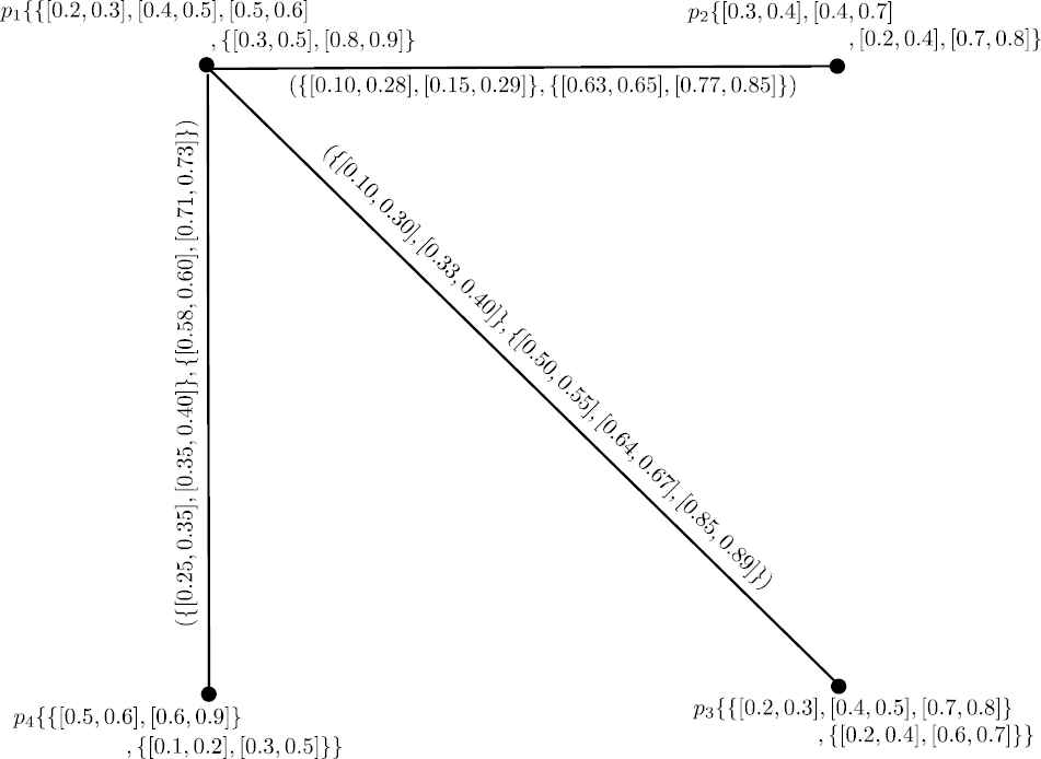
A transport company uses graph to represent their routes. The stations are represented by vertices V={f1,f2,f3,f4} and the routes that connect between a pair of stations are represented by edges E={f1f2,f1f3,f1f4} in the graph. Transport company usually give some choices of route when their customer looks for a ride to a certain destination. There will be several choices which include a connecting (transit-included) ride and direct ride (non-transit ride), as in Figure 1.
Clearly, Ξ̃=(ℑ̃,ℜ̃) is an IV3-RODHFHG. Tabular representation of IV3-RODHFHG is in Table 1:
f1
f2
f3
f4
h̃ℑ̃
{[0.2,0.3],[0.4,0.5],[0.5,0.6]}
{[0.3,0.4],[0.4,0.7]}
{[0.2,0.3],[0.4,0.5],[0.7,0.8]}
{[0.5,0.6],[0.6,0.9]}
ξ(h̃ℑ̃)
0.4250
0.4500
0.4750
0.6500
g̃ℑ̃
{[0.3,0.5],[0.8,0.9]}
[0.2,0.4],[0.7,0.8]}
{[0.2,0.4],[0.6,0.7]}
{[0.1,0.2],[0.3,0.5]}
ξ(g̃ℑ̃)
0.6250
0.5250
0.4750
0.2750
f1f2
f1f3
f1f4
h̃ℜ̃
{[0.10,0.28],[0.15,0.29]}
{[0.10,0.30],[0.33,0.40]}
{[0.25,0.35],[0.35,0.40]}
ξ(h̃ℜ̃)
0.2050
0.2825
0.3375
g̃ℜ̃
{[0.63,0.65],[0.77,0.85]}
{[0.50,0.55],[0.64,0.67],[0.85,0.89]}
{[0.58,0.60],[0.71,0.73]}
ξ(g̃ℜ̃)
0.7250
0.6438
0.6550
Table 1
Tabular representation of an IV3-RODHF vertices and edges.
Now we represent the graph energy under IV q-RODHFH circumstances and investigate its characteristics.
Definition 3.3.
The adjacency matrix A(Ξ̃)=(A(h̃ℜ̃(pipj)),A(g̃ℜ̃(pipj))) of an IV q-RODHFHG Ξ̃=(ℑ̃,ℜ̃) is a square matrix A(Ξ̃)=[aij],aij=(h̃ℜ̃(pipj),g̃ℜ̃(pipj)), where h̃ℜ̃(pipj) and g̃ℜ̃(pipj) indicate the relationship strength and non-relationship strength between pi and pj, respectively.
Definition 3.4.
The adjacency matrix spectrum of an IV q-RODHFHG A(Ξ̃) is described as (Y,Z), where Y and Z are the sets of eigenvalues of ξ(A(h̃ℜ̃(pipj))) and ξ(A(g̃ℜ̃(pipj))), respectively.
Definition 3.5.
The energy of an IV q-RODHFHG Ξ̃=(ℑ̃,ℜ̃) is defined as:
LetΞ̃=(ℑ̃,ℜ̃)be an IVq-RODHFHG andA(Ξ̃)be its adjacency matrix. Ifℶ1≥ℶ2≥…≥ℶnandℸ1≥ℸ2≥…≥ℸnare the eigenvalues ofξ(A(h̃ℜ̃(pipj)))andξ(A(g̃ℜ̃(pipj))), respectively, then:
Therefore Spec(Ξ̃)={(−0.4036,−1.4209),(−0.0045,−0.0029),(0.0045,0.0029),(0.4036,1.4209)}. Now, E(ξ(h̃ℜ̃(pipj))=0.8162 and E(ξ(g̃ℜ̃(pipj)))=2.8476. Therefore, E(Ξ̃)=(0.8162,2.8476).
4. ZAGREB ENERGY OF AN IV q-RODHFHG
This section defines and investigates the first and second Zagreb energy of an IV q-RODHFHG and provides its properties in detail.
4.1. First Zagreb Index and First Zagreb Energy of an IV q-RODHFHG
The first Zagreb index is defined as M1(Ξ̃)=∑pi∈ℑ̃(Ξ̃)dΞ̃2(pi) and satisfies the identity M1(Ξ̃)=∑pipj∈ℜ̃(Ξ̃)(dΞ̃(pi)+dΞ̃(pj)). Further, the closely related quantity known as hyper-Zagreb index is defined as HM(Ξ̃)=∑pipj∈ℜ̃(Ξ̃)(dΞ̃(pi)+dΞ̃(pj))2.
Definition 4.1.
Let Ξ̃=(ℑ̃,ℜ̃) be an IV q-RODHFHG on n vertices. The first Zagreb matrix, Z(1)(Ξ̃)=(Z(1)(h̃ℜ̃(pipj)),Z(1)(g̃ℜ̃(pipj)))=[zij(1)] of Ξ̃ is a n×n matrix defined as:
zij(1)=0ifi=j,dΞ̃(pi)+dΞ̃(pj)if the verticespiandpjof the IVq-RODHFHGΞ̃are adjacent,0if the verticespiandpjof the IVq-RODHFHGΞ̃are non-adjacent.
Definition 4.2.
The first Zagreb energy of an IV q-RODHFHG Ξ̃=(ℑ̃,ℜ̃) is defined as:
Now, ZE(h̃ℜ̃(fifj))=14.6171 and ZE(g̃ℜ̃(fifj))=39.6498. Therefore, ZE(Ξ̃)=(14.6171,39.6498).
For the sake of simplicity, the indicator first will be omitted and we denote the (first) Zagreb matrix by Z(Ξ̃), its (i, j)-element by zij , its eigenvalues by (Φ1,Ψ1),(Φ2,Ψ2)…(Φn,Ψn) and its energy by ZE. Thus, firstly, we put forward the trace of the Zagreb matrices Z(Ξ̃), Z2(Ξ̃), Z3(Ξ̃), and Z4(Ξ̃), i.e., tr(Z(Ξ̃)), tr(Z2(Ξ̃)), tr(Z3(Ξ̃)), and tr(Z4(Ξ̃)). Moreover, the lower and upper bounds for Zagreb energy are obtained by using these equalities.
Lemma 4.1.
Let Ξ̃=(ℑ̃,ℜ̃) be an IV q-RODHFHG on n vertices and Z(Ξ̃)=Z(h̃ℜ̃(pipj)),Z(g̃ℜ̃(pipj)) be the Zagreb matrix of Ξ̃. Then
Therefore, tr(Z2(h̃ℜ̃(pipj)))=∑i=1n∑j∈{1,2,…,n}i∼j(dh̃(pi)+dh̃(pj))2=2∑i,j∈{1,2,…,n}i∼j(dh̃(pi)+dh̃(pj))2=2HM(h̃ℜ̃(pipj)). Similarly, tr(Z2(g̃ℜ̃(pipj)))=2∑i,j∈{1,2,…,n}i∼j(dg̃(pi)+dg̃(pj))2=2HM(g̃ℜ̃(pipj)). Hence tr(Z2(Ξ̃))=2HM(Ξ̃). In addition, if i≠j
Now we determine tr(Z4(h̃ℜ̃(pipj))). Because tr(Z4(h̃ℜ̃(pipj))) = ∥Z2(h̃ℜ̃(pipj))∥F2, where ∥Z2(h̃ℜ̃(pipj))∥F indicates the Frobenius norm of Z(h̃ℜ̃(pipi))2, we obtain
When k=2, we get result ZE(h̃ℜ̃(pipj))≥12HM(h̃ℜ̃(pipj)). Analogously, ZE(g̃ℜ̃(pipj))≥12HM(g̃ℜ̃(pipj)). Hence ZE(Ξ̃)≥12HM(Ξ̃).
4.2. Second Zagreb Index and Second Zagreb Energy of an IV q-RODHFHG
The second Zagreb index, generally denoted by M2(Ξ̃), is defined as:
M2(Ξ̃)=∑pipj∈ℜ̃(Ξ̃)dΞ̃(pi).dΞ̃(pj)
Definition 4.3.
Let Ξ̃=(ℑ̃,ℜ̃) be an IV q-RODHFHG on n vertices. The second Zagreb matrix, Z(2)(Ξ̃)=Z(2)(h̃ℜ̃(pipj)),Z(2)(g̃ℜ̃(pipj))=[zij(2)], of Ξ̃ is represented by a n×n matrix as:
zij(2)=0ifi=j,dΞ̃(pi).dΞ̃(pj)if the verticespiandpjof the IVq-RODHFHGΞ̃are adjacent,0if the verticespiandpjof the IVq-RODHFHGΞ̃are non-adjacent.
Definition 4.4.
The second Zagreb energy of an IV q-RODHFHG Ξ̃=(ℑ̃,ℜ̃) is characterized as:
Now, ZE(2)(h̃ℜ̃(fifj))=6.0455 and ZE(2)(g̃ℜ̃(fifj))=44.3152. Therefore, ZE(2)(Ξ̃)=(6.0455,44.3152).
5. HARMONIC ENERGY OF AN IV q-RODHFHG
This section investigates and defines the Harmonic energy of an IV q-RODHFHG and related properties are provided in detail.
Definition 5.1.
Let Ξ̃=(ℑ̃,ℜ̃) be an IV q-RODHFHG on n vertices. The Harmonic matrix, H(Ξ̃)=(H(h̃ℜ̃(pipj)),H(g̃ℜ̃(pipj)))=[hij], of Ξ̃ is a square matrix defined as:
hij=0wheneveri=j,2dΞ̃(pi)+dΞ̃(pj)whenever the verticespiandpjof the IVq-RODHFHGΞ̃are adjacent,0whenever the verticespiandpjof the IVq-RODHFHGΞ̃are non-adjacent.
Definition 5.2.
The Harmonic energy of an IV q-RODHFHG Ξ̃=(ℑ̃,ℜ̃) is defined as:
Now, HE(h̃ℜ̃(pipj))=11.3221 and HE(g̃ℜ̃(pipj))=4.0877. Therefore, HE(Ξ̃)=(11.3221,4.0877).
First of all, we establish the trace of the Harmonic matrices H(Ξ̃), H2(Ξ̃), H3(Ξ̃), and H4(Ξ̃), i.e., tr(H(Ξ̃)), tr(H2(Ξ̃)), tr(H3(Ξ̃)), and tr(H4(Ξ̃)). Furthermore, the lower and upper bounds for Harmonic energy are determined using these equalities.
Lemma 5.1.
Let Ξ̃=(ℑ̃,ℜ̃) be an IV q-RODHFHG on n vertices and H(Ξ)̃=(H(h̃ℜ̃(pipj)),H(g̃ℜ̃(pipj))) be the Harmonic matrix of Ξ̃. Then
If Ξ̃ is a graph with only isolated vertices, i.e., without edges, then ϒi = 0 for all i=1,2,…,n, and therefore HE(h̃ℜ̃(pipj)) = 0. Since no vertices are adjacent, ∑i∼j2dh̃(pi)+dh̃(pj)=0. If Ξ̃ is a graph with only end vertices, i.e. having degree one, then ϒi = ±dh̃(pi), so the variance of |ϒi|=0,i=1,2,…,n. Thus HE(h̃ℜ̃(pipj))=22n∑i∼j1(dh̃(pi)+dh̃(pj))2.
Analogously, we can show that HE(g̃ℜ̃(pipj))≤22n∑i∼j1(dg̃(pi)+dg̃(pj))2.
Hence
HE(Ξ̃)≤22n∑i∼j1(dΞ̃(pi)+dΞ̃(pj))2.
Theorem 5.2.
LetG̃=(ℑ̃,ℜ̃)be an IVq-RODHFHG onnvertices. IfΞ̃is regular of degree(p,q),p,q>0, then
HE(Ξ̃)=1(p,q)E(Ξ̃).
Proof.
Suppose that Ξ̃ is a regular IV q-RODHFHG of degree (p,q)(p,q>0), i.e., dh̃(p1)=dh̃(p2)=…=dh̃(pn)=p. Then all non zero entries of H(h̃ℜ̃(pipi)) are equal to 1p, implying that H(h̃ℜ̃(pipi))=1pA(h̃ℜ̃(pipi)). Therefore, for all 1≤i≤n
Let Ξ̃=(ℑ̃,ℜ̃) be an IV q-RODHFHG on n vertices. The Randić matrix, R(Ξ̃)=(R(h̃ℜ̃(pipj)),R(g̃ℜ̃(pipj)))=[pij], of Ξ̃ is a square matrix represented as:
pij=0ifi=j,1dΞ̃(pi)dΞ̃(pj)if the verticespiandpjof the IVq-RODHFHGΞ̃are adjacent,0if the verticespiandpjof the IVq-RODHFHGΞ̃are non-adjacent.
Definition 5.4.
The Randić energy of an IV q-RODHFHG Ξ̃=(ℑ̃,ℜ̃) is represented as:
where YR and ZR are the Randić eigenvalues sets of R(h̃ℜ̃(pipj)) and R(g̃ℜ̃(pipj)), respectively.
Definition 5.5.
Let Ξ̃=(ℑ̃,ℜ̃) be an IV q-RODHFHG on n vertices. The general Randić matrix, Rα(Ξ̃)=(Rα(h̃ℜ̃(pipj)),(Rα(g̃ℜ̃(pipj))))=[pij], of Ξ̃ is a square matrix characterized as:
pij=0ifi=j,(dΞ̃(pi)dΞ̃(pj))αif the verticespiandpjof the IVq-RODHFHGΞ̃are adjacent,0if the verticespiandpjof the IVq-RODHFHGΞ̃are non-adjacent.
Definition 5.6.
The general Randić energy of an IV q-RODHFHG Ξ̃=(ℑ̃,ℜ̃) is characterized as:
Now, RE(1∕4)(h̃ℜ̃(pipj))=7.8469 and RE(1∕4)(g̃ℜ̃(pipj))=13.0657. Therefore, RE(1∕4)(Ξ̃)=(7.8469,13.0657).
Theorem 5.3.
LetΞ̃=(ℑ̃,ℜ̃)be an IVq-RODHFHG onnvertices. IfΞ̃is regular of degree(s,t),s,t>0, then
RE(Ξ)̃=HE(Ξ)̃.
Proof.
Suppose that Ξ̃ is a regular IV q-RODHFHG of degree (s,t)(s,t>0), i.e., dh̃(p1)=dh̃(p2)=…=dh̃(pn)=s. Then all non zero entries of R(h̃ℜ̃(pipi)) are equal to 1s, implying that R(h̃ℜ̃(pipi))=1sA(h̃ℜ̃(pipi)). Therefore, for all 1≤i≤n
On the based of the theory of graphs, in this section, we develop a MADM approach with IV q-RODHFNs. Let ℷ={ℷ1,ℷ2,…,ℷn} be a discrete set of alternatives, and Q̌={Q̌1,Q̌2,…,Q̌n} be the set of attributes. Suppose that ℌ̃=(d̃ij)m×n=(h̃ij,g̃ij)m×n is the IV q-RODHF decision matrix, where h̃ij represents a set of degrees that the alternative ℷi meets the attribute Q̌j, and g̃ij represents a set of degrees that the alternative ℷi does not meet the expert’s Q̌j attribute.
The score and accuracy functions based on expected value of IV q-RODHFEs are defined as:
Definition 6.1.
Suppose d̃=(h̃,g̃) is an IV q-RODHFN. Š(d̃)=121+h̃(ς)q−g̃(ς)q is the score function of d̃=(h̃,g̃) and Ȟ(d̃)=h̃(ς)q+g̃(ς)q is the accuracy function of d̃=(h̃,g̃), where
Let d̃i=(h̃i,g̃i)(i=1,2) be any two IV q-RODHFNs, then
if Š(d̃1)>Š(d̃2), then d̃1≻d̃2;
if Š(d̃1)=Š(d̃2), then: (a) if Ȟ(d̃1)=Ȟ(d̃1), then d̃1=d̃2; (b) if Ȟ(d̃1)>Ȟ(d̃2), then d̃1≻d̃2.
In the following, based on the introduced IV q-RODHFGs, a novel MADM approach is proposed to solve this problem.
Step 1.
Determine the scores (based on expected values) utilizing Def. (6.1) of IV q-RODHFEs in an IV q-RODHF decision matrix.
Step 2.
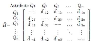
Suppose H̃=(d̃ij)n×n is an IV q-RODHFPR via pairwise comparisons over the attributes Q̌j,j=1,2,…,n, given by the experts. Construct a matrix of an IV q-RODHFPR H̃=(d̃ij)n×n as:
where d̃ij represents the preference of the attribute Q̌i to the attribute Q̌j for all i,j=1,2,…,n.
Step 3.
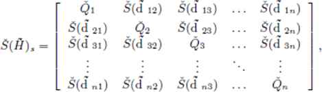
Construct an IV q-RODHFPR Š(H̃) with scores, as follows:
Step 4.
Draw the most favourable digraph for alternative selection attributes whose vertices and directed edges (arcs) portray the considered attributes and the attribute preference, respectively.
Step 5.
Define an appropriate matrix of alternative selection attributes with all of the attributes Q̌i as diagonal elements and their preference Š(d̃ij) as off-diagonal elements.
where Q̌i is the i-th attribute defined by vertex and Š(d̃)ij is the preference of the i-th attribute over the j-th attribute denoted by the edge Q̌iQ̌j of the above matrix’s digraph.
Step 6.
To find an alternative selection index, substitute the values Š(d̃)ij and Q̌j in the alternative selection attributes function.
Step 7.
Rank ℷi(i=1,2,…,m) alternatives as per the alternative index of the selection and pick the best one(s).
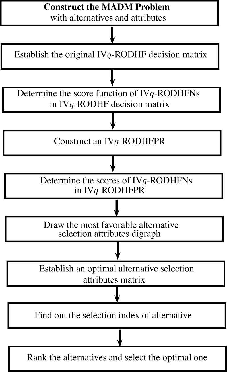
The specific steps of this proposed approach to MADM is depicted in Fig. 4.
Figure 4
The specific steps of the proposed approach to MADM.
6.1. Numerical Example and Comparative Analysis
6.1.1. Assessment of the Performance of search and rescue robots (PSRR)
We use the proposed MADM methodology in this section to determine the PSRR. The PSRR is excellent in emergency cases. In emergency situations, rescue robots took place of the respondents as they were able to take pictures of the scenes and capture certain online streams that can help a lot to understand the seriousness of the situation. Search and rescue robots may be useful to locate casualties or a possible threat in caves, tunnels and the wilderness. The incentive to use these robots of search and rescue is their apediency and completeness of the mission without risks to victims or rescuer.
6.1.2. Numerical example
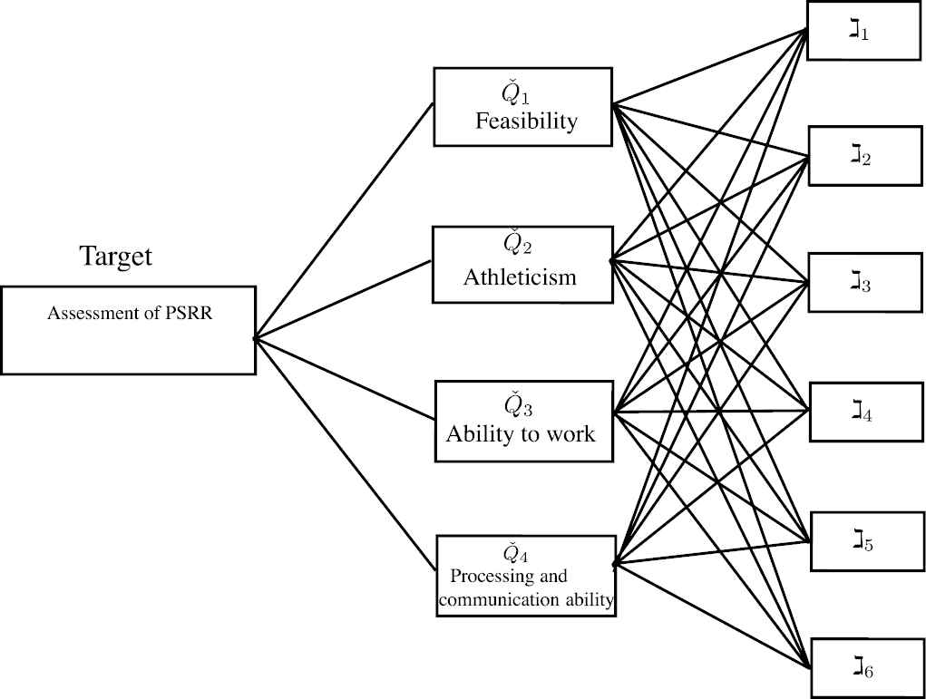
In this example, we address the problem of assessing the PSRR. This example is extracted from [47] where search and rescue robots’ output was tested under IF information. However, only two facts of human opinion have been studied in this environment which leads to lack of information as the degree of abstinence and denial of human opinion is ignored. On the basis of the existing literature [47], the attributes that play an important role in the evaluation of search and rescue robots include Q̌1; feasibility, Q̌2; athleticism, Q̌3; ability to work and Q̌4; processing and communication ability. Let ℷi(i=1,2,…,6) denote the number of search and rescue robots that need to be evaluated. Here the evaluation involves the personal views of the experts that they provide in the manner of a decision matrix that reflects the four attributes.
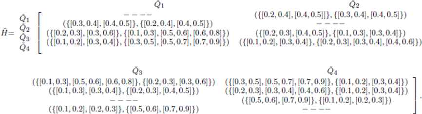
Suppose the experts evaluate the performance of six search and rescue robots ℷi(i=1,2,…,6) according to the four attributes, based on IV q-RODHFNs and the corresponding decision matrix is constructed in Table 2. Figure 5 represents the hierarchical structure of the discussed MADM problem.
Determine the score functions Š(d̃ij)(i=1,2,…,6,j=1,2,3,4) , as shown in Table 3, of the IV4-RODHFEs d̃ij(i=1,2,…,6,j=1,2,3,4) in IV4-RODHF decision matrix.
Step 2.
Preference of attributes is also assigned [48]. Assume the specialists choose the following assignments:
Step 3.
Determine the score functions Š(d̃ij)(i,j=1,2,3,4) of the IV4-RODHFEs d̃ij(i,j=1,2,3,4) in IV4-RODHFPR H̃.
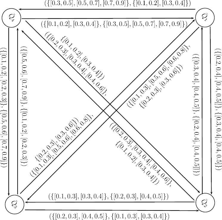
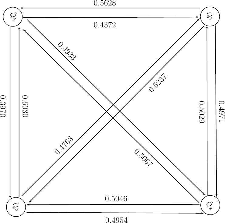
The directed network of the assessment of the PSRR given in Fig. 6, and the directed network of assessment of the PSRR with scores in Fig. 7, indicate the preference of four attributes (digraph’s vertices) Q̌1,Q̌2,Q̌3 and Q̌4. The assessment of the PSRR attributes matrix is attained based on Q̌j(j=1,2,3,4) and d̃ij for each alternative PSRR, where Q̌j is the value of j-th attribute indicated by the PSRR ℷi and d̃ij is the preference of the i-th attribute over j-th attribute.
Step 5.
Substitute the values of Q̌1,Q̌2,Q̌3 and Q̌4 in above matrix H̃, for six search and rescue robots ℷi(i=1,2,…,6) and get
Determine the permanent function values of H̃(i)(i=1,2,…,6), that is, per(H̃(1))=1.4209, per(H̃(2))=1.3864, per(H̃(3))=1.3356, per(H̃(4))=1.5555, per(H̃(5))=1.4051per(H̃(6))=1.5107. The search and rescue robots index values of different search and rescue robots are: ℷ1=1.4209,ℷ2=1.3864,ℷ3=1.3356,ℷ4=1.5555,ℷ5=1.4055,ℷ6=1.5107.
Step 7.
Rank the search and rescue robots ℷ4≻ℷ6≻ℷ1≻ℷ5≻ℷ2≻ℷ3. The search and rescue robot number ℷ4 is therefore the best choice for dealing with emergencies.
Scores
Q̌1
Q̌2
Q̌3
Q̌4
ℷ1
0.3875
0.4942
0.5165
0.5164
ℷ2
0.5000
0.4824
0.3875
0.4954
ℷ3
0.3426
0.4581
0.4845
0.5072
ℷ4
0.5019
0.4968
0.5293
0.5640
ℷ5
0.5135
0.3828
0.4766
0.5192
ℷ6
0.5108
0.5058
0.5032
0.5135
Table 3
IV4-RODHF score function decision matrix.
Figure 6
The directed network of the assessment of the PSRR attributes.
Figure 7
The directed network of assessment of the PSRR attributes with score functions.
6.2. Comparative Analysis
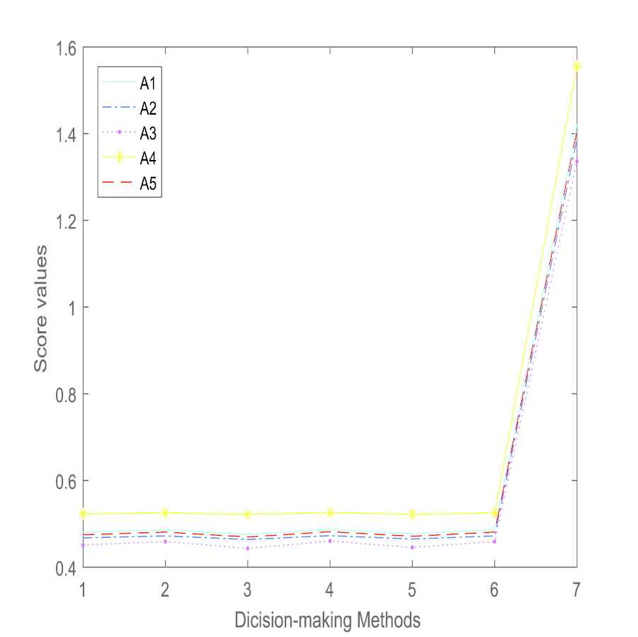
To illustrate the superiority and advantage of our proposed approach, we compare the proposed approach with some existing methods in literature with IV q-RODHFSs. Xu et al. [11] proposed the decision making approach based on MM and dual MM operators with IV q-RODHF information. Wei et al. [49] set forward the decision making method based on Maclaurin symmetric mean (MSM) and dual MSM operators based on q-ROFS. Wei et al. [50] developed the MADM model utilizing Hamy mean (HM) and dual HM operators under DHPF circumstances. We have utilized these approaches to the above illustrative instance and compared the decision results with the developed method of this paper for IV q-RODHFGs. The results of these approaches are summarised in Table 4 and the effects of different methods on the score function and ranking results is shown in Figure 8.
Comparison of score values of alternatives ǐ(i=1,2,3,4,5) of different decision-making methods.
Xu et al.’s [11], and Wei et al.’s [49] methods are based on IV q-RODHFSs and q-ROFSs, respectively. Wei et al.’s [50] method is based on DHPFSs. As DHPFS is a special case of q-RODHFS. That is, when q = 2, then q-RODHFS is converted to DHPFS. Obviously, IV q-RODHFS is progressively more general, and contains more information in the MADM process. Therefore, our developed method provides more general, and powerful information in MADM.
From this comparative study, the outcomes acquired by the proposed approach match with the existing ones which approve the created approach. Subsequently, to tackle the MADM problems, the proposed approach can be reasonably used. The curiosity of this DM approach is that we have built up a MADM model with the interrelated attributes and depicted various connections among the attributes by using the graphical structures with IV q-RODHF data. Our established approach’s merits are summarised as follows:
Evidently, the approach proposed is straightforward and has less data loss and therefore can be easily used in the IVF environment for other MAM problems.
Using graph theory is one of the advantages of the established approach.
More general decision-making scenarios can be accessibly represented by the IV q-RODHFSs of the established technique.
The permanent function has been used to describe the degree to which each alternative is preferred or even more awful than other alternatives.
7. CONCLUSIONS
The IV q-RODHFS can not just manage decision maker’s hesitancy while deciding the MD and NMDs yet in addition gives decision makers more opportunity to express their assessments. The innovative concept of an interval-valued q-rung orthopair dual hesitant fuzzy graphs based on Hamacher operator called IV q-RODHFHGs is put forward in this paper. Certain novel concepts of energy such as Zagreb energy (Zagreb I energy and Zagreb II energy) and Harmonic energy of IV q-RODHFHGs are proposed. We originally modified the existing score function to score function for IV q-RODHFNs, to include the risk preference of the decision maker. Moreover, the proposed concepts of IV q-RODHFHGs were applied to solve the MADM problems with IV q-RODHF information. Finally, we applied the newly proposed concept of IV q-RODHFHGs to the PSRR to demonstrate its effectiveness and validity. Analysis of the comparison has been performed and the superiorities have been shown. The IV q-RODHFHG is a strong method for communicating the hesitation of decision-makers in the MADM process and can explain the fuzziness of networks well. In future, our research work will be extended to: (1) Complex hesitant fuzzy graphs; (2) Complex q-rung orthopair dual hesitant fuzzy graphs; and (3) Complex interval-valued q-rung orthopair dual hesitant fuzzy graphs.
CONFLICTS OF INTEREST
The authors declare no conflict of interest.
AUTHORS' CONTRIBUTIONS
Investigation, Sumera Naz, Muhammad Akram, Samirah Alsulami and Faiza Ziaa; Writing original draft, Sumera Naz , Muhammad Akram and Faiza Ziaa; Writing review and editing, Samirah Alsulami.
23.N.J. Rad, A. Jahanbani, and I. Gutman, Zagreb energy and Zagreb estrada index of graphs, Commun. Math. Comput. Chem., Vol. 79, 2018, pp. 371-386.
24.A. Jahanbani and H.H. Raz, On the harmonic energy and Estrada index of graphs, MATI, Vol. 1, 2019, pp. 1-20.
25.A. Rosenfeld, Fuzzy graphs, L.A. Zadeh, K.S. Fu, and M. Shimura (editors), Fuzzy Sets and their Applications, Academic Press, New York, NY, USA, 1975, pp. 77-95.
TY  - JOUR
AU  - Sumera Naz
AU  - Muhammad Akram
AU  - Samirah Alsulami
AU  - Faiza Ziaa
PY  - 2020
DA  - 2020/12/14
TI  - Decision-Making Analysis Under Interval-Valued q-Rung Orthopair Dual Hesitant Fuzzy Environment
JO  - International Journal of Computational Intelligence Systems
SP  - 332
EP  - 357
VL  - 14
IS  - 1
SN  - 1875-6883
UR  - https://doi.org/10.2991/ijcis.d.201204.001
DO  - 10.2991/ijcis.d.201204.001
ID  - Naz2020
ER  -

 , Samirah Alsulami3, Faiza Ziaa4