

Differential Calculus of Fermatean Fuzzy Functions: Continuities, Derivatives, and Differentials
 , Xin Li1,
 - DOI
- 10.2991/ijcis.d.201215.001How to use a DOI?
- Keywords
- Fermatean fuzzy sets; Continuities; Derivatives; Differentials; Calculus
- Abstract
Fermatean fuzzy sets are an effective way to handle uncertainty and vagueness by expanding the spatial scope of membership and nonmembership of the intuitionistic fuzzy set and the Pythagorean fuzzy set. However, existing studies only analyzed the discrete information and neglected the continuous state of Fermatean fuzzy sets. In this paper, we investigated the properties of continuous Fermatean fuzzy information by firstly proposing Fermatean fuzzy functions, then defining the subtraction and division operations of Fermatean fuzzy functions and discussing their properties. Further, we examined the continuity, derivatives, and differentials of Fermatean fuzzy functions. Effective approximate calculations regarding nonlinear problems in the Fermatean fuzzy environment were provided, and some examples were presented to verify the feasibility and effectiveness of approximate calculations using the Fermatean fuzzy functions.
- Copyright
- © 2021 The Authors. Published by Atlantis Press B.V.
- Open Access
- This is an open access article distributed under the CC BY-NC 4.0 license (http://creativecommons.org/licenses/by-nc/4.0/).
1. INTRODUCTION
Since Zadeh proposed the concept of fuzzy sets [1], many scholars have researched fuzzy set theory. For example, Atanassov [2] proposed the intuitionistic fuzzy sets (IFSs) to characterize uncertainty information according to the degree of membership and nonmembership, providing a basis for other scholars to develop some new fuzzy states of interval IFSs [3,4], intuitionistic 2-tuple linguistic sets [5], intuitionistic trapezoidal fuzzy sets [6,7], intuitionistic normal fuzzy sets [8], intuitionistic uncertain linguistic [9], triangular intuitionistic fuzzy numbers [10–12], linguistic interval-valued intuitionistic neutrosopic fuzzy sets [13], generalized intuitionistic fuzzy Einstein hybrid geometric fuzzy sets [14], interval type-2 fuzzy sets [15], among others. However, IFS and its extensions must meet the criterion that the sum of the degree of membership and nonmembership is less than 1, thereby restricting its application in some decision and information environments [16–18]. For instance, when decision-makers independently evaluate the degree of membership and nonmembership, the sum may be greater than 1 but their quadratic sum would not be greater than 1. To handle this problem, Yager proposed the Pythagorean fuzzy set (PFS) [19,20] to satisfy the quadratic sum of membership and nonmembership degree, i.e., not greater than 1, allowing us to easily infer that the PFS is more useful than IFS in depicting fuzzy information.
After this presentation, PFS-based multi-attribute decision-making (MADM) methods were conducted by many scholars. Peng and Yang [21] investigated the division and subtraction operations of PFS and developed some aggregation operators. Liang et al. [22] combined the TOPSIS and three-way decisions model to present a novel Pythagorean fuzzy decision-making method. Verma and Merigo [23] examined the similarity measures between PFSs. Liu et al. [24] proposed an interval-valued Pythagorean hesitant fuzzy best-worst MADM method to support the product selecting. Rahman and Abdullah [25] developed the family of induced generalized Einstein geometric aggregation operators under interval-valued Pythagorean fuzzy environment. Moreover, Hussian and Yang [26] developed a method for measuring the distance between PFSs using the Hausdorff metric theory. Muhammad et al. [27] developed the ELECTRE I-based MADM method under the Pythagorean fuzzy information. Similarly, Ren et al. [28] presented the TODIM-based MADM method based on the PFSs. Apart from above, Garg [29] established the generalized Einstein operations in PFSs. Yang et al. [30] developed some interval-valued Pythagorean fuzzy Frank power aggregation operators and analyzed its several limiting cases. Meanwhile, Garg [31] defined the neutrality operations in PFSs to aggregate the Pythagorean fuzzy information.
Although IFS and PFS facilitate the resolution of fuzzy decision problems, they still have obvious shortcomings, especially in extremely contradictory decision environments. PFS and IFS are unable to handle a situation where the sum of membership and nonmembership is greater than 1 and the sum of squares is still greater than 1, but the sum of three is less than 1 [32]. For these cases, Senapati and Yager [32] developed the novel concept of Fermatean fuzzy set (FFS), which satisfies the criterion that the sum of the third power of membership and nonmembership must be less than 1. Compared to IFS and PFS, FFS gains a stronger ability to describe uncertain information by expanding the spatial scope of membership and nonmembership. Based on FFS, Wang et al. [33] developed a hesitant Fermatean fuzzy multicriteria decision-making method using Archimedean Bonferroni mean operators, Senapati and Yager [34] proposed Fermatean fuzzy information weighted aggregation operators, and Liu et al. [35] developed a distance measure method for Fermatean fuzzy linguistic term sets. Furthermore, Liu et al. [36] defined a new concept of a Fermatean fuzzy linguistic set and Senapati and Yager [37] developed some new operations between Fermatean fuzzy numbers (FFNs).
However, previous research only focused on how to address the FFS-based decision-making problems with discrete information and did not consider the continuous states of FFS. In many decision-making situations, people need to make decisions in a continuous information environment, such as the diagnosis of the patient's condition, predict the weather and traffic condition, etc. For these issues, some authors have carried out some studies on the continuous fuzzy information. For instance, Lei and Xu [38], Lei et al. [39] defined the intuitionistic fuzzy function (IFFs) to depict the continuous intuitionistic fuzzy information. Based on that, some other scholars analyzed the properties of continuities, derivatives, and differential approximate calculations of IFFs [40,41]. Further, Gou et al. [42] proposed the concept of Pythagorean fuzzy function (PFF) and investigated the continuity and derivability of PFFs. On account of that the deficiencies of IFS and PFS also exist in the differential calculus of IFFs and PFFs, the Fermatean fuzzy function (FFF) and its properties need to be investigated. Therefore, inspired the idea by [38–42], in this work, we treat FFNs as variables to study their continuous states, instead of just treating them as constants. Based on that, we define the novel concept of FFF and examine the properties of continuous Fermatean fuzzy information, such as continuities, derivatives, and differentials. The main aim of this paper is to discuss continuity and calculus theories in the Fermatean fuzzy environment, which provide a method for dealing with nonlinear problems. The main continuations of this paper are summarized as follows:
Defined the novel concept of FFF.
Investigated the properties of continuities, derivatives, and differentials of FFF.
Established a concise decision application framework under continuous Fermatean fuzzy information.
The remaining content of this paper is organized as follows. Section 2 recalls some basic concepts of IFS, PFS, and FFS. The subtraction and division operations on FFNs are defined in Section 3. The definition of FFF and its continuous properties are described in Section 4. The derivative operations between FFFs are defined in Section 5. The differentials of FFFs are introduced in Section 6. And some numerical examples are given to illustrate the properties of FFS in Section 7. Finally, the conclusions are summarized in Section 8.
2. PRELIMINARIES
In this section, we briefly recall some basic concepts about IFS, PFS, and FFS.
Definition 2.1.
[2] With a nonempty set, the form of IFS was defined by Atanassov as
Definition 2.2.
[19] Let
Definition 2.3.
[32] Assuming that
For convenience, we considered
The membership grades related to FFSs are herein referred to as Fermatean membership grades (FMGs).
Definition 2.4.
[32] Let
Definition 2.5.
[32] Let
Theorem 2.1.
[32] Let
Definition 2.6.
[32] Let
Theorem 2.2.
For any FFN
Theorem 2.3.
For any FFN
According to Definition 2.3 and 2.6,
Definition 2.7.
[32] Let
If
If
If
If
If
If
Definition 2.8.
Let
3. SUBTRACTION AND DIVISION OPERATIONS ON FFNs
To further derive the derivative and differential of FFFs, we define the subtraction and division operations based on Definition 2.5 and Gao et al.'s study [43] as follows.
Definition 3.1.
Let
Definition 3.2.
Let
Theorem 3.1.
Let
The following two conditions required proof.
Since
Further,
therefore,
Similarly,
Since
Further,
Moreover,
Therefore, condition (ii) was met, meaning that the result of the subtraction operation of
Theorem 3.2.
If
According to [43] and [44], a novel order relationship based on the addition and subtraction of FFNs is presented as follows.
Definition 3.3.
Let
Definition 3.4.
Let
According to Definition 2.5 and 3.1, the partition relationships between the addition and subtraction regions and between the multiplication and division regions were analyzed, as shown in Figures 1–3.

The addition and subtraction regions.
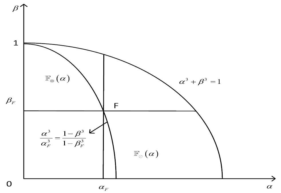
The multiplication and division regions.
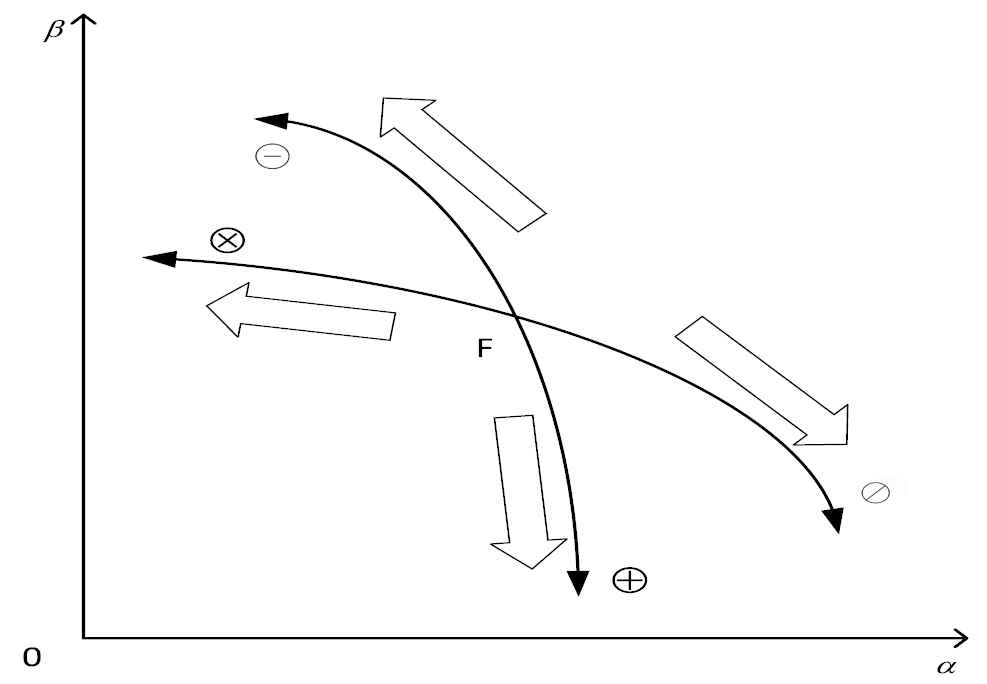
The different change directions with respect to F.
Theorem 3.3.
Let
According Theorem 3.3 and Definition 2.5, we obtained
Theorem 3.4.
Let
If
Proof for (ii).
If
For
Proof for (i).
Proof for (iii).
The others could be proven in a similar way, therefore, the procedures were omitted from explanation.
4. FFF AND ITS CONTINUITY
In this section, we first propose a definition of FFF based on the basic information regarding the FFNs. Besides, we introduce the continuous information of FFF, which plays a fundamental role in calculus. Then, we discuss the calculus properties of FFFs.
Definition 4.1.
The continuous functions of the multivariable were defined as
In addition, we assumed that
Let
The function
According to Definition 2.5, Definitions 3.1, and 3.2, we obtained the following:
Theorem 4.1.
Let
For a fixed
whereFor a fixed
where
Based on the basic properties introduced in Definition 4.1 and Theorem 4.1, the calculus properties of FFFs can be discussed, starting with the continuity of FFFs and considering whether the following limit was suitable for FFFs regarding their operations.
Equation (18) was described as follows:
Definition 4.2.
Therefore,
Definition 4.3.
If Equation (18) is unsuitable for FFFs in their operations, then
Theorem 4.2.
Assuming that
5. THE DERIVATIVE OPERATOR OF FFFs
The derivative operation is an essential concept in calculus, and the essence of the derivative is the local linear approximation of the function through limit operation, which can indicate the rate of change of a function value relative to its variable. Therefore, it can be used as an effective method to calculate the instantaneous rate of change in many fields, such as economics, physics, and medicine.
For this section, we modified classical calculus theories and introduced a definition for the derivative operations of FFFs. A derivate formula of FFF is proposed in this section, allowing us to further discuss some properties of the derivative, such as Chain's law and other operations.
Definition 5.1.
Let
Theorem 5.1.
The uniqueness of the limit showed that if
Theorem 5.2.
Let FFF
In particular, if
For proof, according to Equations (6) and (7), we obtained
We first considered
According to Theorem 4.1, we obtained
Based on Equations (26) and (29), we derived
Thus, the last equal sign in (25) was reasonable.
Hence,
Next, we considered
Thus, according to Equation (21), the above deduction led to
Theorem 5.3.
Equation (20) was necessary to guarantee that
Theorem 5.4.
We found that functions
Theorem 5.5.
In terms of Theorem 3.2,
Definition 5.2.
The FFF
For proof, according to Equation (17), we obtained
For all
Therefore, Equations (20) and (21) were guaranteed.
Furthermore, from Equation (22), we obtained
The basic operations of the derivatives of FFFs are discussed in the following theorems.
Theorem 5.6.
Assuming the existence of FFF derivatives, then,
Then,
For proof, regarding Equation (31),
Since
According to Equation (22), we derived
This is Equation (31).
For Equation (22),
Since
According to Equation (22), we obtained
This is Equation (32).
The proof for Equations (33) and (34) was similar to the proof for Equations (31) and (32), so was omitted from the explanation.
As a direct consequence, we obtained
In terms of Chain's law of derivatives, we obtained the following derivative operations for compound FFFs
Theorem 5.7.
Let
As the first instance of proof,
As the second instance of proof, let
Since,
6. FFF DIFFERENTIALS
In mathematics, a differential operator is an operator defined as a function of the differentiation operation. Differential operators encompass an effective method to estimate function changes based on the proportion of variable variation, which can be regarded as an effective way to linearly approximate nonlinearity problems on the condition that the changes are appropriate. Besides, the FFF differential can be used to estimate the approximate value. For example, decision-makers want to change the value or add some new values after calculation, but the workload of recalculation is too large in some decision-making environments to obtain the accurate results. For this situation, we can use differentiation to estimate the approximate value.
In this section, the intrinsic properties of differential operators in Fermatean fuzzy environment are studied, and the theories of FFFs are discussed. The definition of an FFF differential operator is first discussed, followed by the necessary assumptions needed to ensure an FFF is differentiable. We further propose a differential formula usually used in a variety of applications and numerical calculations.
Definition 6.1.
Let
Theorem 6.1.
Let
As proof, according to Equation (6), we obtained
If the hypotheses in Theorem 5.6 hold true, namely,
Based on Definition 3.2, we deduced that
Next, we compared Equations (40) with (41) to identify whether Definition 6.1 holds true. We explore Taylor's expansion theorem to handle the membership degree, as follows:
In a similar way, we derived
Based on Equations (39–43), we obtained
Therefore, Equation (41) was regarded as Equation (40), i.e.,
By combining all of the above, including Equations (36) and (37)
Theorem 6.2.
If
Based on [44], we proposed an approach approximating a nonlinear FFF in the following corollary:
Corollary 6.1.
Let
As proof, based on Definition 3.2, Equations (35), (38), and (40), we obtained
Corollary 6.2.
If the FFF
The proof of Corollary 6.2 was similar to the proof of Theorem 6.1, so was omitted from explanation.
When comparing Equation (35) with Equation (47), the sign “
7. NUMERICAL EXAMPLES AND APPLICATIONS
In order to illustrate the validity and accuracy of the differential approximate calculation formula in this paper, some numerical examples of the approximation of nonlinear FFF with Fermatean fuzzy continuous information is provided as follows:
Example 7.1.
Let
Based on Definition 2.5 and Theorem 3.4, we derived
Based on Theorem 5.6 and Theorem 6.1, we obtained
According to the result of Equation (49), we can find the validity of the differential approximate calculation formula, then we can further conduct its application as follows:
Example 7.2.
Five FFN decision values were derived using the Fermatean method from five experts, i.e.,
In case some experts wanted to change their preference, we assumed that first expert wanted to change the value of
For simplicity, based on Theorem 5.6, and Theorem 6.1, we assumed
In conclusion, there were tiny differences observed between the results of Equations (51) and (52). Hence, the differential approximate calculation formulae regarding FFFs were effective and feasible.
If the first expert changes the value of
For simplicity, based on Theorem 5.6, and Theorem 6.1, we assumed
We find that there is a big difference between Equations (53) and (54). The reason is the FFWA operator cannot handle extreme cases. So, we further discuss the extreme value situation through the q-ROF interaction Maclaurin symmetry mean (q-ROFIWMSM) operator in [47].
According to the q-ROFIWMSM operator, we obtain the following aggregation value:
If the first expert changes the value of
For simplicity, based on Theorem 5.6, and Theorem 6.1, we assumed
Obviously, there are little differences between Equations (55) and (56). Therefore, the differential approximate calculation formulae regarding FFFs are effective and feasible.
8. CONCLUSION
Considering the continuous Fermatean fuzzy information, we discussed the continuities, derivatives, and differentials of FFF. In it, we firstly proposed the subtraction and division operations between FFNs and discussed their properties, which laid the foundation for further discuss the derivatives and differentials. Then, we defined the concept of FFF and investigated its continuity that plays an important role in calculus. Moreover, we defined the derivatives and differentials of FFFs and examined the algebraic and compound operations of the derivatives of FFFs. Finally, we conducted some examples to verify the feasibility and effectiveness of the approximate calculation on FFFs. Compared to the existing studies, our method is nonlinear with its application in a more expansive range. Besides, the proposed method can address both continuous and discrete information.
In further studies, the elastic coefficients of FFFs and their relationships with the derivatives can be investigated. The inverse operations of the derivatives of the FFFs, such as indefinite integral and definite integral derivatives, can be further examined. Apart from those, the FFF-based decision-making method can be applied to complex uncertainty information decision-making environments, such as the selection of business partners in the supply chain, the prediction of traffic conditions, etc [48–50].
CONFLICTS OF INTEREST
We declare that there are no conflicts of interest regarding the publication of this paper.
AUTHORS' CONTRIBUTIONS
Zaoli Yang: Conceptualization, Funding acquisition, Supervision, Software, Resources, Data curation, Supervision, Writing - review & editing; Harish Garg: Conceptualization, Data curation, Supervision, Software, Resources, Writing - review & editing; Xin Li: Formal analysis, Investigation, Writing - review & editing.
ACKNOWLEDGMENTS
This work was supported in part by the Natural Science Foundation of China (No. 71704007), the Beijing Social Science Foundation of China (No. 18GLC082).
REFERENCES
Cite this article
TY  - JOUR
AU  - Zaoli Yang
AU  - Harish Garg
AU  - Xin Li
PY  - 2020
DA  - 2020/12/22
TI  - Differential Calculus of Fermatean Fuzzy Functions: Continuities, Derivatives, and Differentials
JO  - International Journal of Computational Intelligence Systems
SP  - 282
EP  - 294
VL  - 14
IS  - 1
SN  - 1875-6883
UR  - https://doi.org/10.2991/ijcis.d.201215.001
DO  - 10.2991/ijcis.d.201215.001
ID  - Yang2020
ER  -