
Parameter Identification of Fractional Order Chaotic System via Opposition Based Learning Bare-Bones Imperialist Competition Algorithm
 , Dongge Lei1, Lulu Cai1, Peijiang Li2
- DOI
- 10.2991/ijcis.d.201223.001How to use a DOI?
- Keywords
- Parameter identification; Fractional order chaotic system; Imperialist competition algorithm; Opposition based learning
- Abstract
In this paper, a new method is proposed to identify the parameters of fractional order chaotic system. The parameter identification is achieved by minimizing the mean square error between the states of original fractional chaotic system and those of the estimated one, in which the parameters to be identified are regarded as the optimization variables. To effectively solve the optimization problem, an improved meta-heuristic algorithm, i.e., opposition based learning (OBL) Bare-bones imperialist competition algorithm (OBL-BBICA), is proposed. The proposed OBL-BBICA introduces the OBL and Gaussian sampling into imperialist competition algorithm (ICA) to enhance the exploration ability of ICA, and thus, overcomes the drawbacks of premature phenomena of ICA. OBL-BBICA is adopted to search the optimal parameters of fractional order chaotic system. Experimental results show that the proposed method can accurately identify the parameters of fractional order chaotic system.
- Copyright
- © 2021 The Authors. Published by Atlantis Press B.V.
- Open Access
- This is an open access article distributed under the CC BY-NC 4.0 license (http://creativecommons.org/licenses/by-nc/4.0/).
1. INTRODUCTION
Chaos is an interesting dynamics generated by determined nonlinear differential equations. Chaos is sensitive to initial values of differential equation and exhibits random-like property. Chaos shows great potential in scientific and engineering fields such as information encryption [1], optimization method [2], modeling of economic phenomena [3], chatter prediction [4] etc.
Fractional order calculus (FOC) is a generation of ordinary integer order calculus (IOC). In FOC, the order of differential and integral can be any real numbers. Different from IOC, FOC is global and history dependent. Fractional order differential equations (FODEs) or fractional order models (FOMs) are generalizations of its’ integer counterparts using FOC. FOMs exhibit great superiority in modeling the dynamic behavior of many real systems. Most of important, researchers observed chaos in fractional order systems (FOS) with appropriate orders and parameters [5,6]. The studies of fractional order chaotic system (FOCS) had attracted many researchers’ attention. Parameter identification of FOCS is an important research topic because the precise parameters or orders information is the basics of various applications of FOSC. In the past, several methods had been proposed to identify the parameters and orders of FOCS. In Ref. [7], a synchronization method was proposed to identify the parameters of FOCS. In the proposed method, the parameters of the response system are unknown. The parameter identification is achieved by driving the response system to synchronize the driving system. In Ref. [8], features based artificial neural network (ANN) was proposed to identify the parameters of FOCS. The ANN is used to model the map relationship between the features and parameters of FOCS. Due to the global search ability and flexibility in solving different optimization problems, population based evolution algorithm were also adopted to identify the parameters and orders of FOCS. In Ref. [9], Tang et al. proposed to use differential evolution (DE) algorithm to identify the parameters and orders of commensurate order FOCS. Furthermore, FOCS with unknown initial values and structure are identified in Ref. [10] using DE algorithm. In Ref. [11], the cuckoo search algorithm (CSA) was adopted to identify the parameters of fractional order financial system. In Ref. [12], artificial bee colony (ABC), Grey wolf optimizer (GWO), Whale optimization algorithm (WOA) and ant colony optimizer (ACO) were applied to identify the parameters of fractional order financial chaotic system.
Imperialist competition algorithm (ICA) is also a class of population based evolutionary algorithm. It was proposed by Atashpaz-Gargari and his co-workers in 2007 [13] motivated by socio-politically phenomenon in the world. Compared to other meta-heuristic algorithms, ICA exhibits its competitiveness in terms of convergence rate and global search ability. Since its proposition, ICA had been widely applied to solve different scientific and engineering problems such as ANN training [14], job scheduling [15], controller design [16] etc. Though ICA is successful in solving many problems, however, it also possesses premature phenomena and it is most likely to trap into local optimal when solving complex or high dimensional optimization problem. To overcome this drawbacks, different variants of ICA had been proposed. The chaotic ICA [17,18], Mutation operator based ICA [19], hybrid based ICA [20,21] are representive examples.
In this paper, an new improved ICA is proposed. The proposed method introduces the concept of opposition based learning (OBL) into ICA to enhance the exploration ability of ICA. Meanwhile, the movement of colony toward to imperialist are modified using Gaussian sampling procedure, which borrows from bare-bones particle swarm optimization (PSO). The proposed improved ICA is called as bare-bones imperialist competition algorithm (OBL-BBICA). Then, the proposed OBL-BBICA is adopted to simultaneously identify the parameters and orders of FOCS.
The reminder of this paper is organized as follows. Some basic knowledge that will be used in this paper is introduced in Section 2. In Section 3, the proposed OBL-BBICA is illustrated in details. In Section 4, the identification of FOCS using OBL-BBICA is given. The experimental results are given in Section 5. Finally, the conclusive remarks are presented in Section 6.
2. SOME BASIC KNOWLEDGE
2.1. Fraction Calculus
Fractional calculus means that the order of differential or integral operation can be any real number. It is regraded as a generalization of ordinary integro-differential operator, which is defined as [22]
While the R-L definition is given as [23]:
In this paper, the G-L definition is used to obtain the numerical solution of FOCS. According to Eq. (1), one can obtain the following approximation,
2.2. Opposition Learning
The idea of opposition learning was first proposed by Tizhoosh in 2005 [24]. He thinks that the opposition of current solution may be beneficial for a learning or optimization problem. The advantage of this idea had been proven via several examples such extended genetic algorithm (GA), neural network training. Here, the definition of opposition number is first given.
Definition 1.
(Opposite number) [24] Let
Definition 2.
(Opposite point in the
Definition 3.
(Opposition-based optimization) [24] Let
3. THE PROPOSED OBL-BBICA
3.1. Imperialist Competition Algorithm
Like other evolutionary algorithm, ICA is also a population based meta-heuristic algorithm. Each individual in the population is called “country,” which stands for a candidate solution of a specific optimization problem. These countries are classified into several empires according to their power. In each empire, the powerful country is selected as the imperialist and others are colonies. In the evolutional process, each colony in an empire undergoes assimilation and revolution step to enhance the power of themselves and the whole empire. Then, all the empires in the population compete each other. The empire that succeeds in the competition will become more powerful and takes possession of the colonies of the failures, and the failures will lose their power and ultimately collapse. Finally, only one empire exists and all the countries are colonies of the empire. In this state, each colony has the same position and power as the imperialist and the algorithm converges. The main steps of ICA are stated in the following.
3.1.1. Generating initial empires
In ICA, each country is represented by a
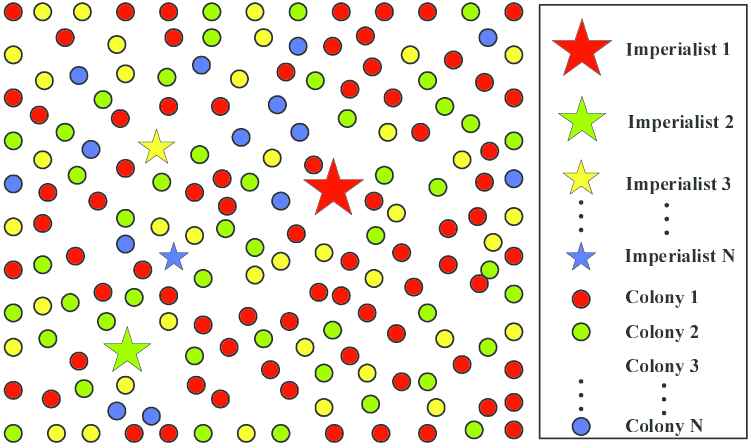
Generating the initial empire.
After initial empires are built, the whole population starts its evolution. The evolution process includes assimilation, revolution and imperialistic competition.
3.1.2. The assimilation process
In this phase, each colony in an empire moves toward the imperialist from its current position. The movement of colony is illustrated in Figure 2, in which the colony moves toward the imperialist by
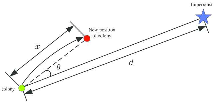
Moving colonies toward their relevant imperialist.
After movement, the cost of a colony maybe better than that of its relevant imperialist. If this case occurs, the imperialist and the colony exchange their positions, see Figure 3. That is to say, the colony become imperialist and the old imperialist become a colony. Then, the algorithm will continue by the new imperialist and then colonies start moving toward this position.
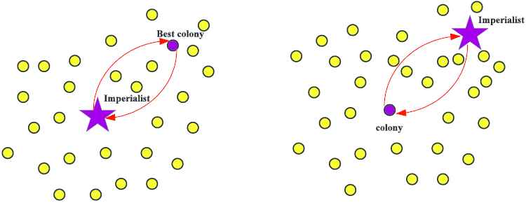
Position exchange between imperialist and colony.
If all the colonies of an empire finish the movement, the empire becomes more powerful. The total power of an empire consists of the power of the imperialist and the colonies. The total power of an empire is calculated as
3.1.3. Imperialistic competition
Once the assimilation process finished, the imperialistic competition takes place between empires, as shown in Figure 4. The purpose of competition is to increase the power of more powerful empires and decrease the power of weaker ones. To do this, one or more the weakest colonies of the weakest empires is picked up and all empires compete to possess these (this) colonies. Each empire has chance to possess the colonies according to its total power. The probability of each empire possessing the colonies is defined as
To assign the above colonies to empires according to the possession probability, a vector
A vector
The empire whose relevant index is maximum in
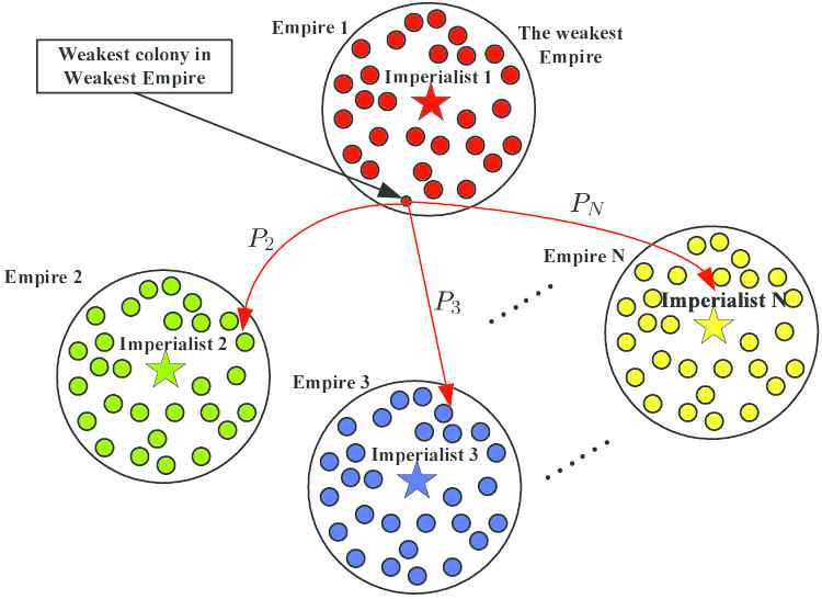
Imperialist competition. The more powerful an empire is, the more likely it will possess the weakest colony of the weakest empire.
In the imperialistic competition, the weaker empire will gradually lose its colonies. If an empire losses all its colonies, it collapses and will be eliminated.
3.1.4. Convergence
After empire competition, beside the most powerful empire, all the other empires will collapse and all the colonies will belongs to this empire. As a consequence, all the colonies alone with the unique imperialist will locate at the same position and have the same costs. In such a condition, the competition is stopped and the algorithm is terminated.
3.2. OBL-BBICA
Although ICA shows great potential in solving different optimization problem, however, it still suffers from a disadvantage, i.e., it converges fast and is easy to trap into a local optimal. To overcome this drawback, opposition learning based BBICA is proposed.
3.2.1. BBICA
BBICA was proposed in [25,26], which borrows the idea of bare-bones PSO. The main steps of BBICA are the same as basic ICA except for the assimilation procedure. In BBICA, the movement of colonies in the assimilation procedure is modified to a Gaussian sampling procedure. Different from Gaussian sampling scheme in [25,26], in this paper, the new position of a colony in an empire is determined as
3.2.2. Enhance BBICA using opposition learning
As stated before, the opposition learning can enhance the performance of most evolutionary algorithms. In this section, the opposition learning is adopted to enhance the performance of BBICA. The improvements are two-folds, i.e., opposition based initialization and opposition based assimilation, which is stated as follows.
Opposition based initialization
The initialization includes the following steps:
Initialize a population
Generates the opposition population
Sort the countries in the union
Select the best
Opposition based assimilation
Assimilation is a key step in ICA. To enhance the exploration ability of ICA, opposition learning is introduced into ICA. Opposition based assimilation is implemented as the following. Suppose there are
For each country in an empire, moving the country to a new position according to Eq. (20).
After all the counties moving to a new position, generate
Calculate the fitness of each country and its opposite counterpart.
Sort the countries and it’s opposition counterpart according to their fitness.
Select the first
4. PARAMETER IDENTIFICATION OF FOCS USING OBL-BBICA
4.1. Problem Statement
Considering a
In the following, the optimization problem (27) is solved via the proposed OBL-BBICA.
4.2. The Procedure of FOCS Parameter Identification Using OBL-BBICA
In this subsection, the parameter vector of FOCS (1) is identified via the proposed OBL-BBICA. The main steps are as follows.
- Step 1:
Determine the parameters of OBL-BBICA, i.e., the number of countries
- Step 2:
Initialization: randomly generate
- Step 3:
According to the generated initial
- Step 4:
Apply the G-L definition to solve the original FOCS and obtain the state vector sequence
- Step 5:
Substitute the value of each country and its opposition country to FOCS and solve the FOCS using G-L definition to obtain the estimated state vector sequence
- Step 6:
Sort the fitness of the
- Step 7:
Select the first
- Step 8:
- Step 9:
For each empire, after each colony update its position, generate the corresponding opposition colony according to Eq. (8).
- Step 10:
For each empire, calculate the fitness of each colony and its opposition counterpart, then sort their fitness in ascending order, and select the first
- Step 11:
For all the empire, perform imperialistic competition.
- Step 12:
Check the converge condition is satisfied? If not, go to Step 8; otherwise, output the position of the imperialist of the final empire as the optimal estimation of parameters.
5. EXPERIMENTAL RESULTS
To demonstrate the effectiveness of the proposed OBL-BBICA in the identification of FOCS, two identification examples are presented in this section. The proposed OBL-BBICA is compared with the original ICA, BBICA and OBL-ICA, genetic algorithm and PSO. The parameters of all the ICAs, GA and PSO referenced in this paper are set as: the size of population is 50 and the maximum number of iteration is 500, other parameters are set to the standard values suggested in [13]. For GA, the other parameter settings are the same as Ref. [9]. For PSO,
5.1. Identification of Fractional Lü System
The first identification example is the fractional Lü system described by the following FODE,
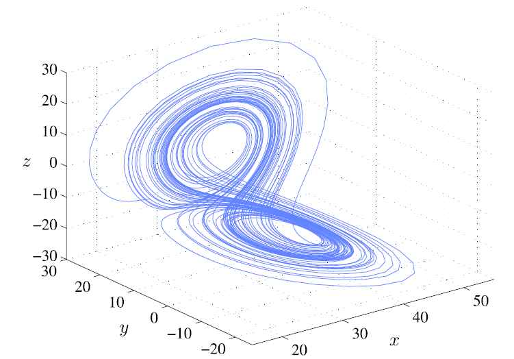
Chaotic behavior of fractional Lü system.
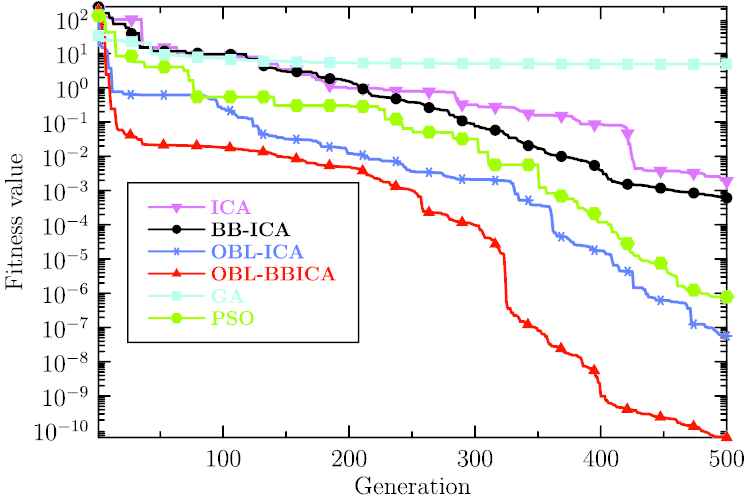
To identify the parameters of the fractional Lü system, the ICA, BBICA, OBL-ICA, OBL-BBICA, GA and PSO all independently run 30 times, and the low and upper limits of each parameter is set to
It can be seen from Table 1 that the identification result of the proposed OBL-BBICA is more accurate than those of ICA, BBICA, OBL-ICA, GA and PSO, which verifies the superior of the proposed algorithm. To see the convergence of ICAs, the evolutionary curve of each algorithm is plotted in Figure 6. Obviously, the convergence of the proposed OBL-BBICA is faster than other three algorithms, and the final mean square error of state vector is the smallest. This further verifies the superior of the proposed method.
| Algorithm | Parameters | Best | Worst | Mean |
|---|---|---|---|---|
| ICA | 24.9725 | 20.0000 | 24.3843 | |
| 3.0025 | 1.0000 | 2.8447 | ||
| 27.9748 | 26.3635 | 27.9290 | ||
| 0.7999 | 0.7120 | 0.7876 | ||
| BBICA | 24.9825 | 22.3161 | 24.8594 | |
| 3.0008 | 1.4402 | 2.9479 | ||
| 27.9853 | 28.4400 | 27.9721 | ||
| 0.7999 | 0.7410 | 0.7977 | ||
| OBL-ICA | 25.0001 | 24.3658 | 24.8130 | |
| 3.0000 | 1.0000 | 2.8316 | ||
| 28.0001 | 27.2807 | 27.9694 | ||
| 0.8000 | 0.7895 | 0.7960 | ||
| OBL-BBICA | 25.0000 | 24.0000 | 24.9687 | |
| 3.0000 | 3.1161 | 2.9881 | ||
| 28.0000 | 27.0070 | 27.9904 | ||
| 0.8000 | 0.7583 | 0.7990 | ||
| GA | 25.4505 | 25.3762 | 24.9828 | |
| 2.4823 | 2.9341 | 2.9894 | ||
| 28.6225 | 28.3208 | 28.4562 | ||
| 0.7322 | 0.5952 | 0.6345 | ||
| PSO | 24.9820 | 27.1558 | 25.2282 | |
| 2.9988 | 4.0323 | 3.2259 | ||
| 27.9992 | 25.9544 | 27.4148 | ||
| 0.7999 | 0.9991 | 0.8386 |
Identification result of fractional Lü system.
Evolution curve of each algorithm for identifying fractional Lü system.
5.2. Identification of Fractional Volta System
A fractional order Volta’s system [27] described by
| Algorithm | Parameters | Best | Worst | Mean |
|---|---|---|---|---|
| ICA | 19 | 20.0415 | 18.9844 | |
| 11 | 11.7143 | 10.9779 | ||
| 0.73 | 0.5 | 0.7353 | ||
| 0.99 | 0.9958 | 0.9898 | ||
| BBICA | 19 | 19.7541 | 19.0147 | |
| 11 | 11.6523 | 10.9567 | ||
| 0.73 | 0.5124 | 0.7397 | ||
| 0.99 | 0.9957 | 0.9988 | ||
| OBL-ICA | 19 | 20.0415 | 18.9629 | |
| 11 | 11.7143 | 10.9677 | ||
| 0.73 | 0.5 | 0.7393 | ||
| 0.99 | 0.9958 | 0.9897 | ||
| OBL-BBICA | 19 | 19 | 19 | |
| 11 | 11 | 11 | ||
| 0.73 | 0.73 | 0.73 | ||
| 0.99 | 0.99 | 0.99 | ||
| GA | 19.0077 | 23.4061 | 19.7648 | |
| 11.0206 | 9.4645 | 11.5674 | ||
| 0.7245 | 0.8407 | 0.7584 | ||
| 0.9800 | 0.9160 | 0.9643 | ||
| PSO | 19.0520 | 18.2618 | 18.9261 | |
| 11.0084 | 10.1743 | 10.9174 | ||
| 0.7300 | 0.9000 | 0.7470 | ||
| 0.9920 | 0.9863 | 0.9896 |
Identification results of fractional Volta system.
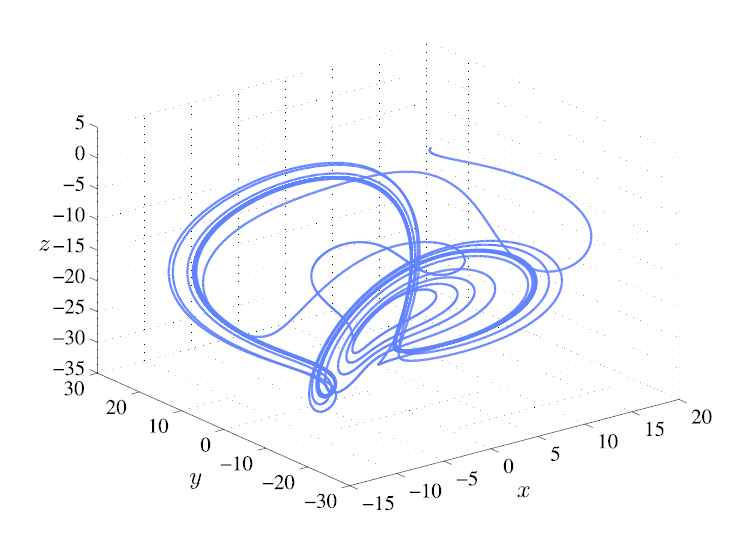
Chaotic behavior of fractional Volta system.
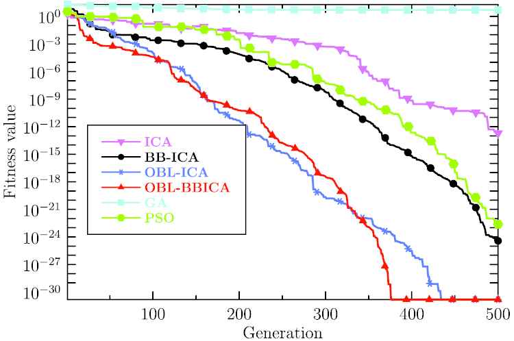
Evolution curve of each algorithm for identifying fractional Volta system.
6. CONCLUSION
In this paper, an improved ICA algorithm, i.e., OBL-BBICA is proposed to solve the parameter identification problem of FOCS. The proposed OBL-BBICA integrates the OBL and Gaussian sampling into ICA to enhance the exploration ability of ICA. The proposed algorithm is used to simultaneously identify the parameters and orders of FOCS via minimizing the mean square error between original system state vector and that of the estimated system. Identification results show that the proposed OBL-BBICA can achieve more accurate identification results than ICA, BBICA, OBL-ICA, GA and PSO verifies the effectiveness of the proposed algorithm.
CONFLICT OF INTEREST
The authors declare no conflict of interest.
AUTHORS' CONTRIBUTIONS
Ting You conceives the idea of the paper and writes the draft of the manuscript. Dongge Lei implements the OBL-BB ICA algorithm. Lulu Cai solves the fractional order chaotic system. Peijiang Li revises the manuscript.
ACKNOWLEDGMENT
This work was sponsored in part by Basic Public Welfare Project of Zhejiang Province of China (LGG18E050003, LGG21F030002).
REFERENCES
Cite this article
TY  - JOUR
AU  - Ting You
AU  - Dongge Lei
AU  - Lulu Cai
AU  - Peijiang Li
PY  - 2020
DA  - 2020/12/29
TI  - Parameter Identification of Fractional Order Chaotic System via Opposition Based Learning Bare-Bones Imperialist Competition Algorithm
JO  - International Journal of Computational Intelligence Systems
SP  - 453
EP  - 460
VL  - 14
IS  - 1
SN  - 1875-6883
UR  - https://doi.org/10.2991/ijcis.d.201223.001
DO  - 10.2991/ijcis.d.201223.001
ID  - You2020
ER  -