
Feature Subset Selection Based on Variable Precision Neighborhood Rough Sets

- DOI
- 10.2991/ijcis.d.210106.003How to use a DOI?
- Keywords
- Rough sets; Variable precision neighborhood rough sets; Attribute reduction; Feature selection; Neighborhood systems
- Abstract
Rough sets have been widely used in the fields of machine learning and feature selection. However, the classical rough sets have the problems of difficultly dealing with real-value data and weakly fault tolerance. In this paper, by introducing a neighborhood rough set model, the values of decision systems are granulated into some condition and decision neighborhood granules. A concept of neighborhood granular swarm is defined in a decision system. Then the sizes of a neighborhood granule and a neighborhood granular swarm are also given. In order to enhance the fault-tolerant ability of classification systems, we define some concepts of granule inclusion, variable precision neighborhood approximation sets and positive region. We propose a variable precision neighborhood rough set model, and analyze its property. Furthermore, based on the positive region of a variable precision neighborhood, we give the significance of an attribute and use it to select feature subsets. A feature subset selection algorithm to the variable precision neighborhood rough sets is designed. Finally, the feature selection algorithm is carried out on the UCI datasets, and the selected features are tested by the support vector machine (SVM) classification algorithm. Theoretical analysis and experiments show that the proposed method can find the effective and compact feature subsets, which have abilities of fault tolerance.
- Copyright
- © 2021 The Authors. Published by Atlantis Press B.V.
- Open Access
- This is an open access article distributed under the CC BY-NC 4.0 license (http://creativecommons.org/licenses/by-nc/4.0/).
1. INTRODUCTION
The classical Rough Set Theory (RST) proposed by Pawlak [1] refers to the whole study objects as a domain. An equivalence relation is used to granulate the domain into several exclusive equivalence classes, called information granules, which are employed in describing the arbitrary concepts in the domain. At present, the RST has been widely used in the fields of attribute reduction [2–5], feature selection [6–9], gene selection [10,11] and classification [12–15], etc. However, as an effective granular computing model, the RST is only suitable for dealing with discrete data. It cannot directly process continuous data, which seriously affects the areas of practical applications. For the disposing of continuous data, we can discretize the continuous data. But this transformation may result to an information loss, and the classification accuracy largely depends on a particular discretization method. In order to solve the problem, the neighborhood RST [16–18] is introduced to granulate these continuous data and some neighborhood granules are constructed for the convenient analyzing and processing real-value data. The neighborhood RST is intuitive, which can directly handle continuous or real-value data without discretization. Compared with classical RST, it eliminates the discretization process and extends an application scope of the Pawlak RST.
Yao [19] initially proposed the neighborhood RST and Hu et al. [20] developed its applications in a classification field. It has been widely used in attribute reduction [21–24], feature selection and extraction [25–27], classification and clustering [28–30], gene selection [31–33], image processing [34,35] and other fields. The neighborhood RST uses the concept of neighborhood positive region. The objects, that their condition granules are completely contained in their decision granules, form the neighborhood positive region. Different neighborhood parameters make the neighborhood positive regions different. The smaller of the neighborhood parameter and the finer neighborhood granule is. Then the neighborhood positive region becomes larger. The neighborhood positive region also relates to the number of attributes. While attributes are gradually increased, the neighborhood granules become smaller. Then the neighborhood positive region becomes larger. If the neighborhood parameter of a neighborhood classification system is fixed, then the neighborhood positive region is also unchanged. The attribute reduction in a neighborhood system refers to the deletion of redundant attributes in the case of preserving the same neighborhood positive region. However, when some noise are added to a neighborhood system, the neighborhood positive region is changed, which affects the accuracy of a classification. For example, a condition granule is completely contained in a decision granule, and when a noise is added, the condition granule may be partially included in the decision granule. Therefore, it is necessary to consider the circumstance of granule partial-inclusion under a noisy condition. The variable precision RST proposed by Ziarko [36], is a rough set model with fault-tolerant ability. It can overcome the limitation of classical RST with the hard-to-process noisy data. It is an informational filtering, which persists in some correct information with a great extent and ignores the noisy information. The classification precision can be controlled by a variable factor of the positive region. The variable precision RST has been widely used in many fields such as decision analysis [37], process control [38], data clustering [39] and attribute selection [40].
Feature selection [41–45] also called feature subset selection or attribute selection, refers to selecting
The main innovative work of this paper is as follows: (1) In order to enhance the fault-tolerant ability of classification systems, we define some concepts of granule inclusion, variable precision neighborhood dependence and approximation sets. (2) Based on these terminologies, a variable precision neighborhood rough set model is proposed, which is suitable to deal with real-value and noisy data. (3) Furthermore, we prove the monotonicity of variable precision neighborhood dependence with increasing features and a feature subset selection algorithm to the variable precision neighborhood rough sets is designed.
The remainder sections are structured as follows: An introduction to neighborhood granulation of classification systems is presented in Section 2. In Section 3, the granule inclusion degree is introduced. Then we propose a variable precision neighborhood rough set model. In Section 4, we propose a feature selection method based on variable precision neighborhood rough sets and design an algorithm for feature subset selecting. In Section 5, for contributing to understand our proposed method, we carry out some experiments in decision systems. Finally, this paper is concluded with some discussions and remarks in Section 6.
2. NEIGHBORHOOD GRANULATION OF CLASSIFICATION SYSTEMS
The RST proposed by Pawlak, a mathematician of Poland, is one of the most widely used models in classification systems. In a machine learning field, huge amounts of real-value data need to be discretized, but the discretization process easily leads to a loss of classification information. Aiming at the limitation of Pawlak RST, a neighborhood RST is introduced to granulate these real-value data. In RST, an equivalence class is regarded as a granule. As for neighborhood RST, neighborhood granules are constructed.
Definition 1.
[20] Let
Definition 2.
[20] Let
where
Definition 3.
Let
If
The values on decision features in classification systems are symbolic data. Therefore, the samples are divided into equivalent classes on the decision features. The neighborhood parameter sets zero, so these samples are granulated into equivalent granules, which are called decision equivalent granules, and they are expressed as
From the above definitions, we can see that a neighborhood granule is degenerated into an equivalent granule when the neighborhood parameter is 0. So the equivalent granule is a special neighborhood granule. The neighborhood granular swarm is a collection of neighborhood granules.
Property 1.
The neighborhood granule
Definition 4.
Let
The
Definition 5.
Let a classification system be
where
Definition 6.
Let a classification system be
It is easy to know that the size of neighborhood granular swarm holds the property:
Definition 7.
[20] Let a classification system be
The order couple
Proposition 1.
Let a classification system be
If
If
Proof.
Since
For
3. VARIABLE PRECISION NEIGHBORHOOD ROUGH SETS
In 1993, Ziarko proposed the variable precision RST [36], which is a generalization of the classical RST and it endures certain classification error rates. However, the variable precision RST can only deal with symbolic or discrete data, which cannot directly handle a large number of symbolic or continuous data in real world. To overcome the deficiency, we introduce neighborhood rough sets, while relaxing the classification accuracy, and propose a variable precision neighborhood rough set model.
Definition 8.
Let
The granule inclusion degree reflects an inclusion relation between two granules. A granule is essentially a set. Figure 1 illustrates a variation for the granule inclusion degree. Suppose
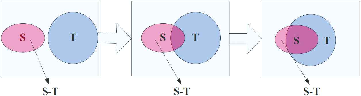
Illustration for the granule inclusion degree.
Example 1.
Suppose a domain
Let a classification system be
Proposition 2.
Let a classification system be
If
If
Proof.
It is known from the Proposition 1, if
Similarly, it is easily proved by the Proposition 1. If
Definition 9.
Let a classification system be
The variable precision neighborhood lower approximation set of
The variable precision neighborhood boundary region of
The variable precision neighborhood negative region is defined as
Apparently for any
Definition 10.
Let a classification system be
The variable precision neighborhood dependence is similar to the variable precision positive region, which reflects the variation of classification accuracy.
Proposition 3.
Let a classification system be
If
If
Proof.
From
From
According to the Proposition 3, we can draw the following conclusions:
Proposition 4.
If
Proposition 5.
If
Proposition 6.
If
The Proposition 4 shows that the classification accuracy is increasing with the growing of features. It is not strictly monotonously increasing, so it may grow to a certain extent, the accuracy of classification no longer changing. Therefore, some features can be gradually selected so that the classification accuracy of these features has been increased to the same classification accuracy of all features. The Proposition 5 shows that the classification accuracy is decreasing with the increasing value of a granulation parameter. Because the process of granulation will increase noise, the larger the value of granulation parameter is, the more noise will be added and the accuracy of classification will decrease. The Proposition 6 shows that the accuracy of classification increases while the threshold of variable precision reduces. Therefore, it is necessary to consider reducing the threshold of the variable accuracy so as to improve the classification accuracy when the noise induced by the granulation parameter increases. The above analysis shows that the variable precision neighborhood rough set model is more robust to the classification systems and can handle the data containing noise.
4. FEATURE SUBSET SELECTION BASED ON VARIABLE PRECISION NEIGHBORHOOD ROUGH SETS
The information entropy, mutual information, rough entropy and knowledge granularity induced by equivalence relations measure the roughness of knowledge and reflect the classification ability of a decision system. However, these measures are suitable to deal with symbolic data. As for real-value data, we should find new methods. From the definition of variable precision neighborhood dependence, we put forward the concept of variable precision neighborhood reduction for real-value and noisy data in classification systems. Furthermore, a feature subset selection algorithm based on variable precision neighborhood rough sets is designed.
4.1. Feature Reduction Based on Variable Precision Neighborhood Rough Sets
Definition 11.
Let a classification system be
A redundant feature provides useless or even spurious classification information. We delete the feature from a classification system, so a more compact and concise feature representation is appeared. It will reduce the dimension and complexity of a big data system.
Definition 12.
Let a classification system be
The first condition means that the selected features and the whole features have the same classification accuracy; the second condition ensures that the selected feature subset does not have redundant features.
From the above analysis, it is known that the variable precision neighborhood dependence reflects the classification ability of a feature subset. And according to the Proposition 4, the variable precision neighborhood dependence monotonically increases with the growing of the features. Therefore, the significance of a feature can be defined based on the variable precision neighborhood dependence.
Definition 13.
Let a classification system be
The significance of a feature represents a change of the variable precision neighborhood dependence, before and after the feature is deleted. The threshold of variable precision shows the tolerance to the noise data.
4.2. Feature Subset Selection Algorithm Based on Variable Precision Neighborhood Rough Sets
From the Propositions 3 and 4, we know that the positive region and dependence of variable precision neighborhood are monotonic. Therefore, we can use the deleting or adding method to select the features. According to the definition of the variable precision neighborhood reduction, we propose a feature subset selection algorithm based on the variable precision neighborhood rough sets. Following the significance of feature as a heuristic information, a bottom-up feature subset selection algorithm is designed.
Algorithm 1: Algorithm VPNRS. A heuristic algorithm to feature selection based on variable precision neighborhood rough setsInput: A classification system C S = ( U , A , D ) δ ∈ [ 0 , 1 ] 0 . 5 ≤ α ≤ 1
Output: A feature reduction RED.
(1): Initialization:
(2): while (
(3):
(4): for each
(5):
(6): for each
(7): Computing the condition neighborhood granule
(8): Computing the decision granule
(9): Computing the granule inclusion degree by
(10): If
(11): End for
(12):
(13): Computing the variable precision neighborhood dependence
(14): If
(15):
(16): End if
(17): End for
(18):
(19): Computing
(20): If
(21):
(22):
(23): If
(24):
(25): End if
(26): End if
(27): End while
(28): Return
In steps 6 and 7, achieving neighborhood granules costs O(
5. EXPERIMENTAL RESULTS
In this paper, some experiments are tested on four UCI datasets, which are shown in Table 1.
Experimental datasets.
Due to the different value ranges of the datasets in the table, the datasets need to be normalized and preprocessed. We use the maximum-minimum method to ensure that all data are transformed into data between 0 and 1. The maximum–minimum normalization is defined as
Experimental results are compared from two aspects. One is the redundancy of selected feature subsets, and the other is the classification accuracy of reduced feature subsets. In the experiments, the values of neighborhood parameter start from 0.05 to 0.5, while their intervals are 0.05 and a total of 10 times are tested. In this paper, the algorithm needs to set the variable precision threshold, which is tested from 0.5 to 1 with an interval of 0.05, and there are 10 kinds of accuracy are changed. First, the feature subset selection (feature reduction) is performed using a variable precision neighborhood rough set model. And then the classification experiments are performed on the selected feature subsets. The experimental dataset is randomly divided into ten parts, of which nine parts are used for training and the remaining one part for testing. The dataset is tested with the LIBSVM classifier developed by Professor Lin Chih-Jen.
5.1. Redundancy Comparison of Feature Reduction
The simplification of a feature reduction is measured by redundancy, and the redundancy is expressed as follows:
Among them,
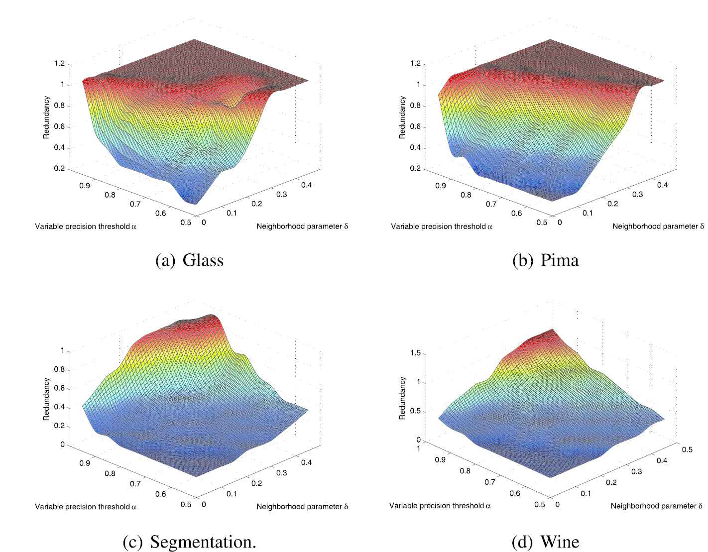
Redundancy comparisons of different datasets.
From the Figure 2(a), for the Glass dataset, when the neighborhood parameter
From the Figure 2(b), for the Pima dataset, when the neighborhood parameter
From the Figure 2(c), for the Segmentation dataset, the neighborhood parameter
From the Figure 2(d), for the Wine dataset, when the neighborhood parameter
From the above analysis, we can see that the smaller the neighborhood parameter is, then the smaller the reduction subset redundancy is and the better the reduction effect is. The smaller the variable precision threshold is, then the smaller the reduction subset redundancy is and the better the reduction effect is. Conversely, the larger the neighborhood parameter is, then the larger the reduction subset redundancy is and the worse the reduction effect is. The bigger the variable precision threshold is, then the larger the redundancy of the reduction subset is and the worse the reduction effect is. At the same time, this is consistent with the principle of Propositions 5 and 6. When the neighborhood parameter becomes bigger, the noise increases. According to the Proposition 5, the classification accuracy is reduced, and more features are needed to describe the dataset. When the variable precision threshold is smaller, according to Proposition 6, the classification accuracy increases, and fewer features can describe the dataset.
5.2. Comparison of Classification Accuracy
The smaller the redundancy, the less the number of features used for a classifier, which is beneficial to speed up the training of the classifier. However, the classification accuracy may be reduced and the effect of classification is not ideal when the selected features are less. Only when the selected feature subset satisfies the two conditions with small redundancy and high accuracy of classification, it is an ideal feature subset. Firstly, we get multiple feature subsets under different neighborhood parameter values and different thresholds, and then test the classification results of these feature subsets. The classifier is LIBSVM, and the experimental results are shown in Figure 3.
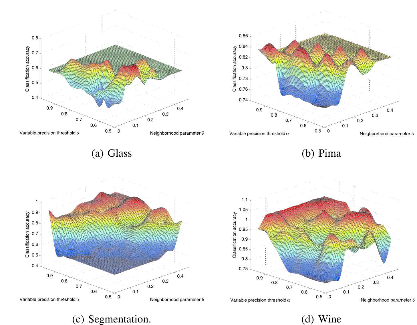
Classification accuracies of different datasets.
From the Figure 3(a), for the Glass dataset, when the neighborhood parameter sets 0.15 and the variable precision threshold sets 0.55, 0.6, and 0.7, the classification accuracy reaches the maximum value with 0.7143. When the neighborhood parameter sets 0.2 and the variable precision threshold sets 0.55, the maximum classification accuracy reaches 0.7143. When the neighborhood parameter sets 0.1 and the variable precision threshold sets 0.7, the classification accuracy reaches the minimum value with 0.4286.
From the Figure 3(b), for Pima datasets, the classification accuracy has 9 maximum values, mainly concentrated on a diagonal line of the plane formed by neighborhood parameters and variable precision thresholds. They are scattered in points with large neighborhood parameter values and small variable precision values, or with small neighborhood parameter values and large variable precision values. The minimum classification accuracy is distributed on the plane with small neighborhood parameter values and small variable precision values at the same time.
From the Figure 3(c), for Segmentation dataset, the classification accuracy has 3 maximum values, scattered in
From the Figure 3(d), for Wine datasets, the points of maximum classification accuracy are numerous, mainly concentrated on a striped line with the variable precision value setting 1 and the neighborhood parameter ranging in 0.1–0.5. The points of minimum classification accuracy are distributed in a striped line with the small neighborhood parameter values and the variable precision threshold ranging in 0.55–0.8.
From the previous experiments, it is known that the simplification effects of feature subsets are better when the neighborhood parameter values and the variable precision thresholds are small. However, as shown in the Figure 3, the classification accuracies are smaller when the neighborhood parameter values and the variable precision thresholds are small. Therefore, the simplification of a feature subset is relevant to the performance of a classification. Meanwhile, from the Figure 3, we can see that when neighborhood parameter values and variable precision thresholds are large, there are many features for classification, but the accuracy of classification is not the best. Because that the neighborhood granulation will bring much noise to the datasets. When the neighborhood parameter value becomes larger, the noise is increased. Although the features are more, the noise is added due to the increasing of neighborhood parameter values, so the classification accuracy is affected. From the Proposition 6, we can see that the decreasing of the variable precision threshold can improve the classification accuracy. Since the noise introduced by a granulation process affects the classification accuracy, we can improve this situation by decreasing the threshold of variable precision, which counteracts the influence of the added noise. Therefore, it is necessary to adjust two values of neighborhood parameter and variable precision threshold at the same time, and select the appropriate features. It will be a good classification performance.
5.3. Comprehensive Comparisons of Redundancy and Classification Accuracy
The experiments in this subsection are compared from two aspects: redundancy of the selected features and their classification accuracies. In general, the classification accuracy is more important than redundancy. So we use the golden split point to set their weights. Suppose the redundancy of a feature subset is
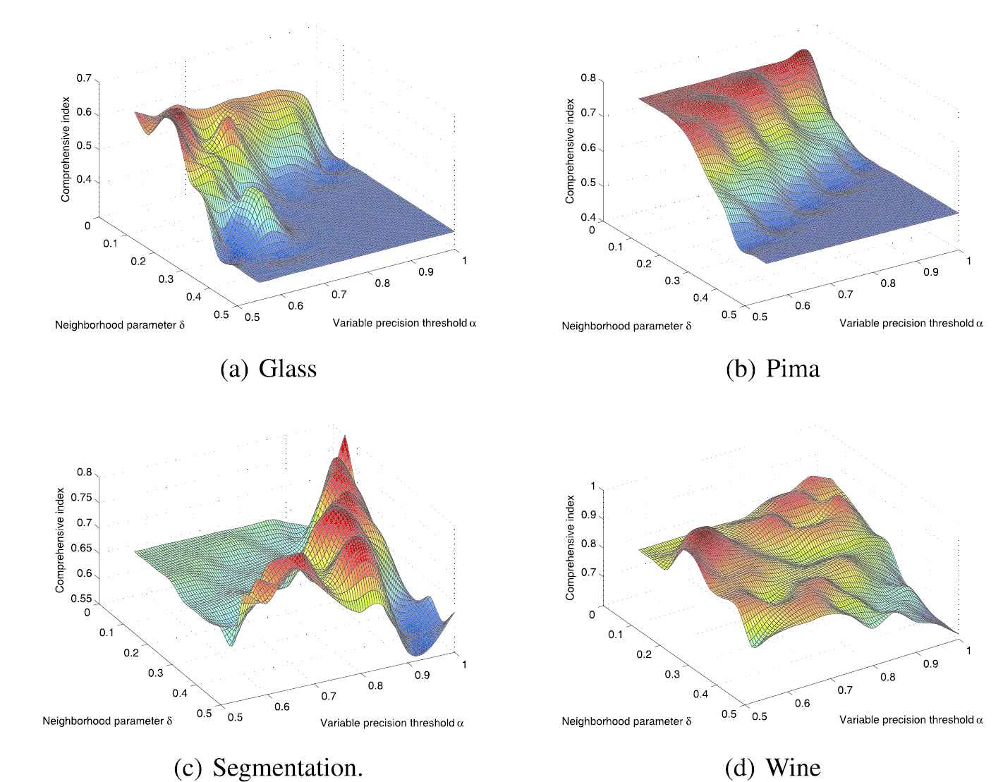
Comprehensive comparisons of different datasets.
From the Figure 4(a), for the Glass dataset, there are 3 maximum values of the comprehensive index, which are distributed on the points
From the Figure 4(b), for the Pima dataset, there are 4 maximum values of the comprehensive index, which are distributed on the points
From the Figure 4(c), for the Segmentation dataset, there is 1 maximum value of the comprehensive index, which is distributed on the point
From the Figure 4(d), for the Wine dataset, there are 5 maximum values of the comprehensive index, which are distributed on the points
In summary, the maximum values of comprehensive index are mainly distributed on the points of smaller neighborhood parameter values. As for the variable precision threshold, it is not very sensitive. The smaller the neighborhood parameter is, the smaller the noise introduced. Therefore, the comprehensive performance of classification accuracy and simplification is not very sensitive to the variable precision threshold under the condition of low noise. The minimum values of the comprehensive index are mainly distributed on the points where the neighborhood parameter values and the variable precision thresholds are both large. If the neighborhood parameter value is large, the noise introduced is much, which indicates that under the condition of much noise, the comprehensive performance of classification accuracy and simplification is more sensitive to the variable precision threshold. At this time, we need to decrease the threshold of variable precision, so that the performance of classification accuracy and simplification is improved.
In order to verify the advantage of variable precision neighborhood rough sets (VPNRS) in processing noisy data, we add Gaussian noise with (0,0,0.004), where the mean is 0, the variance is 0 and the noise amount is 0.004. We compare VPNRS with Hu's neighborhood rough sets (NRS) [17] on these noisy data using K-nearest neighbor (KNN) and SVM classifiers. First, the NRS and VPNRS are utilized for feature selection, and then the KNN and SVM are used for classification experiments to compare their classification accuracies. The results are shown in Table 2.
| Datasets | NRS + KNN | NRS + SVM | VPNRS + KNN | VPNRS + SVM |
|---|---|---|---|---|
| Glass | 65.12 |
66.72 |
66.35 |
65.35 |
| Pima | 79.26 |
78.39 |
80.02 |
79.37 |
| Segmentation | 85.12 |
86.04 |
86.07 |
87.39 |
| Wine | 91.16 |
92.13 |
91.23 |
93.67 |
Classification accuracies of UCI datasets with Gaussian noise.
As it can be seen from the Table 2, for the noisy data, the classification accuracies of VPNRS on both classifiers are higher than those of NRS, indicating that our proposed algorithm has obvious anti-noise ability.
6. CONCLUSIONS
Aiming at the problem of traditional rough sets hardly dealing with real data, the neighborhood rough set granulation is introduced to construct some condition neighborhood granules and decision equivalent granules in decision systems. The size of a granule is defined, the inclusion relation between a condition granule and a decision granule is analyzed, and a variable precision neighborhood rough set model based on the inclusive relation is proposed. Furthermore, the model is used to select feature subsets and a feature subset selection algorithm based on this model is designed. The experimental results show that the new proposed feature subset selection method can remove redundant features in decision systems. The method provides a simplified feature subset for the classifier and simultaneously maintains a good classification performance. It has certain robustness, and can handle the dataset containing noise. In the future work, we can apply the feature subset selection method proposed in this paper to the dimensionality reduction of big data systems.
CONFLICT OF INTEREST
We declare that we have no conflict of interest.
AUTHORS' CONTRIBUTIONS
Yingyue Chen: Conceptualization, methodology, software, validation, formal analysis, data curation, writing - original draft, project administration, funding acquisition, supervision, writing - review and editing, investigation, visualization, resources. Yumin Chen: Visualization, writing - review and editing.
FUNDING
This work is funded by the National Natural Science Foundation of China (grant number 61976183), the Natural Science Foundation of Fujian Province (grant number 2019J01850).
ETHICAL APPROVAL
This article does not contain any studies with human participants or animals performed by any of the authors.
REFERENCES
Cite this article
TY  - JOUR
AU  - Yingyue Chen
AU  - Yumin Chen
PY  - 2021
DA  - 2021/01/12
TI  - Feature Subset Selection Based on Variable Precision Neighborhood Rough Sets
JO  - International Journal of Computational Intelligence Systems
SP  - 572
EP  - 581
VL  - 14
IS  - 1
SN  - 1875-6883
UR  - https://doi.org/10.2991/ijcis.d.210106.003
DO  - 10.2991/ijcis.d.210106.003
ID  - Chen2021
ER  -