
An Efficient CNN with Tunable Input-Size for Bearing Fault Diagnosis
 , Jean Jiang2, Xinnian Guo3, Lizhe Tan4
- DOI
- 10.2991/ijcis.d.210113.001How to use a DOI?
- Keywords
- Bearing fault diagnosis; Deep learning; CNN; STFT
- Abstract
Deep learning can automatically learn the complex features of input data and is recognized as an effective method for bearing fault diagnosis. Convolution neuron network (CNN) has been successfully used in image classification, and images of vibration signal or time-frequency information from short-time Fourier transform (STFT), wavelet transform (WT), and empirical mode decomposition (EMD) can be fed into CNN to achieve promising results. However, the CNN structure is complex and not efficient enough for different datasets. Furthermore, it is less efficient to process the input data by WT and EMD than by STFT. In this work, the low bound for input size of 2D data is analyzed by considering the relationship between the characteristic vibration frequencies and the window size of STFT to guide the determination of the minimum input size. Then a general adaptive CNN structure for different datasets is designed. According to the experimental results for four datasets, the proposed method is universal and the parameter settings can be guided by the low bound of input size. Surprisingly, all classification accuracies for the four datasets can achieve 100% in ten times of independent run without redesigning the CNN structure.
- Copyright
- © 2021 The Authors. Published by Atlantis Press B.V.
- Open Access
- This is an open access article distributed under the CC BY-NC 4.0 license (http://creativecommons.org/licenses/by-nc/4.0/).
1. INTRODUCTION
Condition-based maintenance (CBM), which is also referred to as Prognostics and Health Management (PHM), is a maintenance strategy that can monitor the health condition of machinery in real time and make an optimal maintenance decision based on the condition monitoring information. Henriquez et al. [1] pointed out that CBM usually involved four stages: data acquisition, signal processing, decision support system, and fault diagnosis/prediction. Rai and Upadhyay [2] considered that CBM had three main components, i.e., condition monitoring, health prognosis, and fault diagnosis, of which condition monitoring was the basic component. The condition monitoring component can collect relevant information about the machine condition, including vibration signals, motor current signals, acoustic emission signals, and more recently, stray flux [3]. Health prognosis aims to predict the remaining useful life (RUL) of machinery based on the historical and ongoing degradation trends obtained from condition monitoring information [4]. Fault diagnosis is a process of typifying the damage status through detection, isolation, and identification by using the data collected from continuous health monitoring on the rotating machinery. Here, diagnosis can be regarded as a posterior event analysis [2].
In industrial factories, rolling element bearings (REBs) are the most commonly used machine elements in almost all kinds of rotating machinery, and the health conditions of REBs have considerable impacts on machines. According to a literature review, 45%–55% of broken machines are caused by bearing faults. Hence, condition monitoring and fault diagnosis of bearings are significant tasks in industrial production [2,5].
In general, fault diagnosis methods can be classified into model-based, signal-based, knowledge-based, and hybrid/active ones [6]. Among them, the knowledge-based methods, which are also named as data-driven methods, require a large volume of historical data to establish the fault models for the systems without priori known models or signal patterns [7]. A conventional data-driven method usually consists of three stages, including handcrafted feature design, feature extraction/selection, and model training. Normally, handcrafted feature design is based on the signal processing methods such as Fourier transform (FT), short-time Fourier transform (STFT), wavelet transform (WT), wavelet package transform (WPT), Hilbert–Huang transform (HHT), and empirical mode decomposition (EMD) [8–10]. After a set of features are appropriately designed, they can be fed into some shallow machine learning algorithms such as EMD + SVM [10], HHT + SVM [11], DWT + KNN [12], WPT + KNN [13], and WT + Naive Bayes (NB) [14].
Except for signal processing-based methods, image processing methods are also widely used in many existing studies. Chong converted 1D vibration signals into 2D gray-level images, and the significant features were successfully extracted from vibration signals through the scale invariant feature transform (SIFT) algorithm to generate faulty symptoms [15]. Kang and Kim proposed a 2D gray-level image representation method based on Shannon wavelets, and the image textures could be extracted by generating global neighborhood structure map. Then multiclass SVMs were successfully used for identifying faults in the induction machine [16]. Lu et al. proposed a conversion from signals to images using bi-spectrum technology and t-SNE was used to reduce the dimension of the features extracted by SURF. Then a probabilistic neural network was used for image classification [17].
However, it requires a great deal of human labor and domain knowledge to design features artificially [18]. It is noticed that deep learning can automatically learn complex features of input data. On account of this, deep learning has been considered as an effective method to overcome the above drawbacks.
LeCun et al. first designed a convolution neuron network (CNN) and optimized the model using an error-gradient algorithm. Due to its unique ability of maintaining initial information regardless of shift, scale, and distortion invariance, CNNs have been widely used in image classification [19,20]. There are two type of CNNs in fault detection. One is 1D CNN, and the other is 2D CNN. Ince et al. [21] and Eren [22] applied 1D CNN to real-time motor fault diagnosis. Abdeljaber et al. used 1D CNN for real-time structural damage detection [23]. As for 2D CNN, Guo et al. [24] proposed a hierarchical learning rate adaptive deep CNN (ADCNN) to accomplish fault diagnosis and severity, in which the first layer was based on classical LeNet5 models. Jia et al. [25] used stacked auto encoder (SAE) to learn the useful information from the obtained frequency spectra of rotating machinery. Liu et al. [26] employed stacked sparse auto encoder (SSAE) to automatically extract the fault features of sound spectrograms using STFT, where softmax regression was adopted as the method for classifying fault modes. Wang et al. [27] used wavelet scalogram images as input data into CNN to detect faults within a set of vibration data. Similarly, three time-frequency analysis methods, i.e., STFT, WT, and HHT, were used to generate image representation of raw signals as input into CNN [9]. These methods designed three repetitive CCP layers, and each CCP layer contained two consecutive convolution layers without a pooling layer between them. By this way, vibration signals could be normalized and transformed to vibration images. Further, Wen et al. [7] fed these vibration images into CNN that consisted of four successive convolution and pooling layers for image classification. Similarly, Hoang and Kang [5] designed a CNN structure consisting of two successive convolution and pooling layers to process vibration images and realize image classification.
From the above literature review, conventional and deep learning methods both use images as input data. Hence, it is a general idea to feed 2D or image data into CNN for fault diagnosis. Although many related studies have achieved successful results, there are still many issues that need to be handled. First, most studies directly use vibration signals as image data and cannot capture the frequency information that is important to nonstationary signals [5,7]. Second, although STFT, WT, and HHT can be used to generate spectrum or scalogram images, these color images scaled by bilinear interpolation as the input of CNN may cause efficiency problems [9,27]. Lastly, the design of network structure is still an intractable issue. The CNN structure is too complex because of too many convolution layers [7,9], and different CNN structures or parameters are required to be redesigned according to different datasets.
As we know, STFT is a simple and easy transformation method that can transform time domain signals into time-frequency domain. Thus, it is more efficient than WT, HHT, and EMD. In this study, we use STFT with nonoverlap rectangle window to obtain the power spectrum. The window size is tunable and can be guided through theoretic analysis according to different application situations. Then an efficient and general CNN with tunable input size is proposed for bearing fault diagnosis (CNN-T), which is suitable for many different datasets without any change of CNN structure.
The main contributions of this work can be summarized as follows:
A novel method is proposed to guide the determination of the minimum input size. Because a minimum window size in STFT needs to be determined to keep the information of modulated signals by fault defection and short pulse in time domain, a tunable parameter W with low bound is proposed under the guidance of theoretic analysis, which considers the relationship between the characteristic vibration frequencies and the window size of STFT. After STFT, the normalized power spectrum is used as the input into CNN.
A universal CNN is proposed and successfully applied to four datasets with the same CNN structure, and the proposed CNN can achieve 100% classification accuracy over ten times of independent run.
Through experiments on four datasets, the parameter settings of W can be guided by its low bound, which can improve the application efficiency of the proposed method.
The rest of this paper is organized as follows: Section 2 describes the details of our method including the framework of CNN-T, the design principles of STFT with the low bound W through the theoretical analysis, and the model of CNN. In Section 3, comparison experiments with four datasets are conducted, and the results are presented and analyzed. Finally, Section 4 gives some conclusions and suggests topics for future research.
2. OUR PROPOSED METHOD
In this study, a general CNN with tunable input size W based on STFT (CNN-T) is proposed for bearing fault diagnosis in Figure 1. The raw signals are randomly segmented to many signal frames with W*W points, which can be taken as a function of data augmentation to increase the number and diversity of samples. Of course, W*W can be replaced with W*H. Here, for simplicity, we just use one parameter, i.e., W = H.
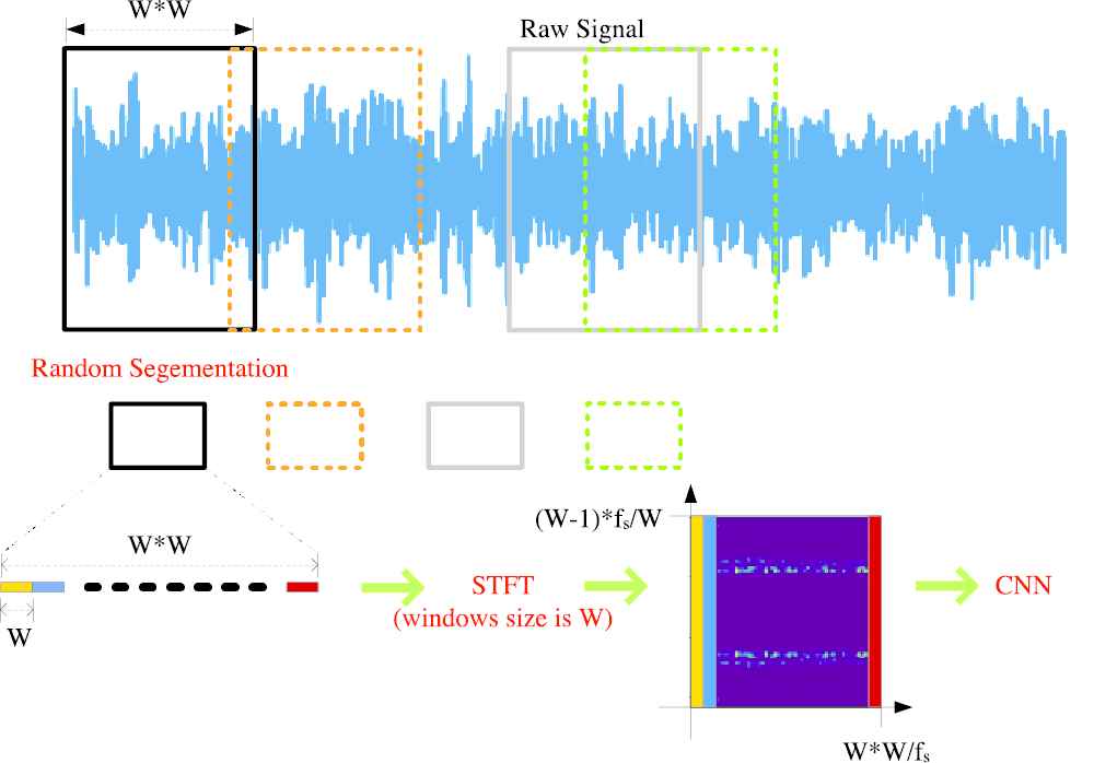
Framework of convolution neuron network (CNN)-T.
After segmentation, each signal frame is processed by STFT. The signal frame is split into W pieces of short data frame, and each data frame is processed by FFT. When it is finished, the power spectrum with time-frequency information can be obtained.
Finally, the power spectrum matrix is normalized and fed into a general CNN for training or identifying. The CNN structure is applied to four datasets without any change of the CNN structure. It should be noted that the coefficient matrix, instead of the spectrum image, is the real data fed into CNN in our proposed method.
2.1. Random Segmentation and STFT with Guided W
When a raw signal arrives, the conventional STFT splits the signal into many frames with fixed window size and overlap size as shown in Figure 2a. By contrast, our proposed method can randomly extract a segmentation of the signal before STFT as shown in Figure 2b. By comparing Figures 2a and 2b, it can be seen that the interval between two segments is different. The conventional STFT has a fixed signal frame overlapping, while our method does not. Hence, our method can be used for data augmentation in deep learning, thus increasing data quantity and obtaining more diversity of spectrum information.
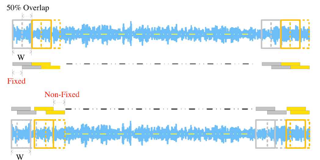
Different segmentation methods.
For clarity, the notations used in the following context are listed in Table 1. According to Fourier series analysis, the coefficients of Fourier series expansion of the periodic signal
| Notation | Description |
|---|---|
| Sampling frequency | |
| Sampling interval | |
| Fundamental period of a periodic digital signal |
|
| Fundamental frequency of |
|
| Fundamental angular frequency of |
|
| The number of samples within the fundamental period of |
|
| The number of harmonics corresponding to the harmonic frequency of |
|
| The number of short data frames or the number of points in one short data frame | |
| Index of short data frame | |
| The number of balls in one bearing | |
| Contact angle of bearing | |
| Shaft speed | |
| Ball diameter | |
| Pitch diameter | |
| Outer race fault frequency | |
| Inner race fault frequency | |
| Ball fault frequency | |
| Cage fault frequency |
Information about notations used.
This transformation is then applied to stationary signals, the properties of which do not evolve over time. When the signal is non-stationary, the signal is multiplied by the window size and truncated into short data frames. By analyzing these short data frames, the output of successive STFTs can provide a time-frequency representation of the signal [28].
In this study, to improve the performance, the rectangular window with a size of W and no overlap size is used in Equation (3). The STFT divides an input signal, which has L data points in Equation (4), into W data frames according to the rectangular window, and then performs FFT on each data frame with W data points as shown in Equation (5).
After STFT, Equation (7) computes the normalized power spectrum for the input of CNN, where p is the collection of
Since STFT uses a fixed window size, if a small window size is adopted, some information such as short pulse or low frequencies may be lost. Hence, a minimum W needs to be determined to keep the information of short pulse in time domain. In addition, when the rolling element hits one fault on the bearing, the vibration signal can be modulated by corresponding frequencies, and the modulated signal caused by the fault conveys some diagnostic information. Based on this, the number of sample points in one segmentation W*W should be large enough to keep this information in one segmentation. For example, in Figure 3, W*W should be greater than the number of data

Modulated vibration signal caused by the fault.
The time interval between these two peaks can be estimated according to the characteristic vibration frequencies, which are calculated by the following Equations (8–13) [8,22]. The outer race fault frequency, the inner race fault frequency, the ball fault frequency, and the cage fault frequency are given by Equations (8–11) respectively. Considering W*W should be greater than the number of data in
2.2. A General CNN Model
The proposed CNN structure is given in Figure 4, and further details are given in Table 2. Three successive convolution and pooling layers are used to extract high-level features. The ReLU is taken as the activation function. The max pooling layer is used for preserving the maximum coefficients because these coefficients contain the main information of fault features.
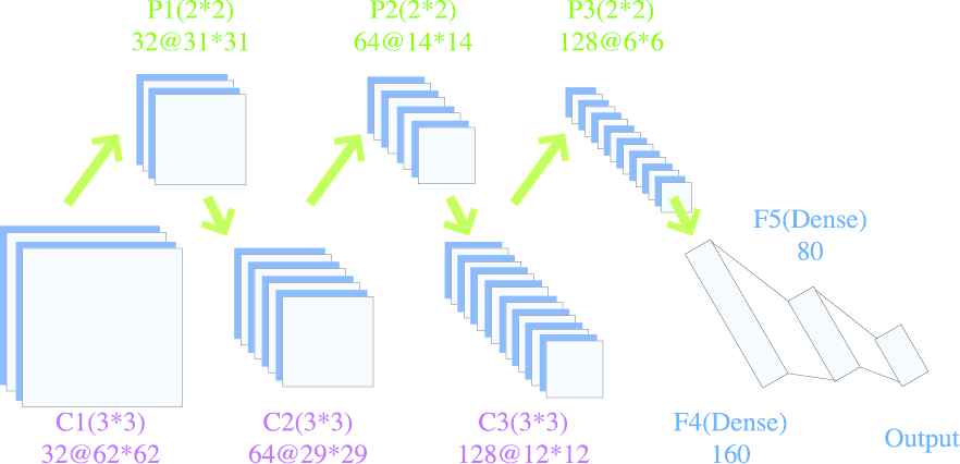
The proposed convolution neuron network (CNN) structure (suppose W = 64).
| Layer Name | CNN Models (Kernel Filter, Activation Function, Strides, Padding) |
|---|---|
| C1 | Conv (32*3*3, ReLU, 1, None) |
| P2 | Maxpool (2, 2, 1) |
| C2 | Conv (64*3*3, ReLU, 1, None) |
| P2 | Maxpool (2, 2, 1) |
| C3 | Conv (128*3*3, ReLU, 1, None) |
| P3 | Maxpool (2, 2, 1) |
| F4 | Dense (160, ReLU) |
| F5 | Dense (80, ReLU) |
| Output | Dense (Clsass_Num, Softmax) |
Detailed information of convolution neuron network (CNN).
Let the kernel size, the padding size, and the stride step be F, P, and S, respectively. Then, the output size can be given by
Suppose that the input data matrix has a size of W*W with W = 64, and then the output size of the first convolution layer is
The loss function uses the categorical cross entropy in Equation (15), in which N is the number of data samples, M is the number of classes,
The optimizer is the Adam method because its hyper-parameters have intuitive interpretations and basically require little tuning [30].
3. EXPERIMENT
In this section, our proposed fault diagnosis method is conducted on four fault diagnosis datasets, i.e., the famous Case Western Reserve University's (CWRU) bearing dataset [31], the famous Machinery Failure Prevention Technology (MFPT) society bearing fault dataset [32], the self-priming centrifugal pump (SPCP) dataset, and the axial piston hydraulic pump (APHP) dataset [17]. In each experiment, let the default batch size be 100, and the number of epochs be 50. All these results are obtained by ten times of independent run with one GPU, Keras, and tensorflow. Let Pt be the proportion of the training data in the whole dataset, and the default value of Pt is 0.8. The classification accuracy is the result obtained by using the corresponding test dataset.
3.1. CWRU Bearing Dataset
As a standard public dataset, vibration data are recorded under various engine loads (0–3 hp) at 1730, 1750, 1772, and 1797 revolutions per minute (rpm). The motor shaft bearings have faults in different depths (none, 0.007, 0.014, 0.021, 0.028 inches), and the fault location includes the inner race, the rolling element, and the outer race.
Table 3 gives the data of the samples of CWRU bearing dataset. As can be seen, all these data, without considering the different revolving speeds, have one normal class and 11 fault classes or 15 fault classes. In this experiment, about 10000 data samples are randomly extracted from the raw data file. Here, the data with 12 classes are used.
| 12 Classes |
16 Classes |
||
|---|---|---|---|
| Type | Number | Type | Number |
| Normal | 624 | Normal | 624 |
| 07-OR | 1872 | 07-OR12 | 624 |
| 07-OR3 | 624 | ||
| 07-OR6 | 624 | ||
| 07-Ball | 624 | 07-Ball | 624 |
| 07-IR | 624 | 07-IR | 624 |
| 14-OR | 624 | 14-OR6 | 624 |
| 14-IR | 624 | 14-IR | 624 |
| 14-Ball | 624 | 14-Ball | 624 |
| 21-OR | 1872 | 21-OR12 | 624 |
| 21-OR3 | 624 | ||
| 21-OR6 | 624 | ||
| 21-IR | 624 | 21-IR | 624 |
| 21-Ball | 624 | 21-Ball | 624 |
| 28-IR | 624 | 28-IR | 624 |
| 28-Ball | 624 | 28-Ball | 624 |
Samples of Case Western Reserve University (CWRU) bearing dataset.
3.1.1. Signal vibration image and STFT image
Figure 5 gives the vibration signal images used by Refs. [5,7] and spectrum images used by our method. Most of them are easier to be classified by human eyes than the vibration images transformed from raw signal data, whereas the two groups of images (14-IR/21-OR and 07-OR/21-Ball/21-IR) require to be carefully observed.
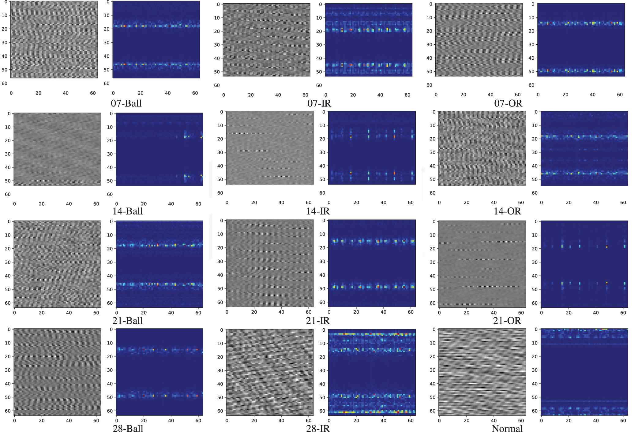
Different images of Case Western Reserve University (CWRU) dataset.
3.1.2. Comparison results
There are many different CNN-based methods, such as CNN-VibrationImage [7], ADCNN [24], CNN-STFT [9], CNN-Wavelet [9], and 1D-2 LAYER CNN [33]. Besides, deep recurrent neural network (DRNN) [34], sparse filter [35], optimized deep belief network with PSO (DBN-PSO) [36], DBN-based HDN [37], and SVM [10] are also used as deep learning methods. In this experiment, CNN-T is compared with shallow machine learning and other deep learning methods, and the results are given in Table 4.
| Method | Average Accuracy | Number of Classes |
|---|---|---|
| CNN-T (W = 96) | 100 | 12 |
| CNN-T (W = 64) | 99.89 | 12 |
| DRNN [34] | 96.53 | 12 |
| CNN-VibrationImage [7] | 99.79 | 10 |
| ADCNN [24] | 98.1 | 10 |
| Sparse filter [35] | 99.66 | 10 |
| CNN- Wavelet 96×96 [9] with CNN [27] | 99.8 | 4 |
| CNN-STFT 96×96 [9] | 99.5 | 4 |
| 1D-2 LAYER CNN [33] | 99.75 | 4 |
| DBN-PSO [36] | 87.45 | - |
| DBN Based HDN [37] | 99.03 | 4 |
| SVM [10] | 87.45 | - |
Comparison results of different methods with Case Western Reserve University (CWRU) dataset (Pt = 0.8, %).
It can be seen that our method CNN-T (W = 96) can achieve an accuracy of 100% in ten times of independent run. Furthermore, the number of classes to be classified is 12, which is more than other methods except DRNN (which has an accuracy of 96.53% for 12 classes). Hence, our method is more efficient than many state-of-art methods, e.g., CNN-VibrationImage (99.79% for 10 classes), Sparse filter (99.66% for 10 classes), CNN-Wavelet (99.8% for 4 classes). The main reason is that the vibration images in Figure 5 are more difficult to be identified than the spectrum images used by our method. Moreover, for other similar CNN-based methods, their complex CNN structure is one factor that leads to their low efficiency.
3.1.3. Sensitivity with samples and W
W signal frames (with different values of W = 32, 64, 96) are extracted from the raw data file, and each frame is processed by FFT separately. The results are shown in Figure 6.
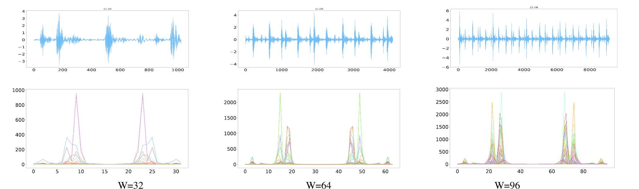
Frequency information with FFT for Case Western Reserve University (CWRU) data set (21-OR).
According to Equation (13) and characteristic vibration frequencies given in Ref. [38],
It is noted that when W = 32 < 46.12 in Figure 6, the obtained STFT amplitude spectrum has low-frequency resolution due to the small size of W and the information of the lowest frequency component may be lost. To further evaluate the effects of different parameters, some experiments with different W values (W = 32, 64, 96) and Pt values (Pt = 0.1, 0.5, 0.8) are conducted, and the results are given in Table 5.
| W | Pt | Min | Max | Mean | Std |
|---|---|---|---|---|---|
| 96 | 0.8 | 100.00 | 100.00 | 100.00 | 0.00 |
| 96 | 0.5 | 99.96 | 100.00 | 99.99 | 0.01 |
| 96 | 0.1 | 98.34 | 99.50 | 98.97 | 0.35 |
| 64 | 0.8 | 99.60 | 100.00 | 99.89 | 0.15 |
| 64 | 0.5 | 99.66 | 99.98 | 99.84 | 0.10 |
| 64 | 0.1 | 98.42 | 99.44 | 98.99 | 0.29 |
| 32 | 0.8 | 99.60 | 99.85 | 99.69 | 0.07 |
| 32 | 0.5 | 99.16 | 99.56 | 99.39 | 0.14 |
| 32 | 0.1 | 94.22 | 96.54 | 95.25 | 0.76 |
Classification accuracies with different parameters (%).
It can be seen from Table 5 that the classification accuracy is proportional to W and Pt. The reason is that more training samples are beneficial to CNN and that more signal frames (a larger W value) can capture more time-frequency information. Furthermore, the results are not sensitive to W and Pt except the situation of an accuracy of 100%.
In Table 5, when W = 96 and Pt = 0.8, an accuracy of 100% is achieved with Std = 0. Furthermore, with the increase of W, lower Pt can achieve higher accuracy than lower W and higher Pt. For example, when W = 96 and Pt = 0.5, the accuracy is 99.99%, which is higher than 99.89% when W = 64 and Pt = 0.8.
3.2. MFPT Bearing Dataset
This famous MFPT dataset is made up of four sets of bearing vibration data including a baseline set, three outer race faults (ThreeOR), seven additional outer race (SevenOR) faults, and seven inner race faults (SevenIR). These data are sampled at 48828 Hz for 3 s in each file. There are also additional data files in the MFPT dataset, but they are not used in our experiment. 10000 data samples shown in Table 6 are randomly extracted from the raw data file.
| Type of Fault | Number of Samples |
|---|---|
| Baseline | 1500 |
| ThreeOR | 1500 |
| SevenOR | 3500 |
| SevenIR | 3500 |
Samples of MFPT bearing dataset.
3.2.1. Signals, vibration images, and STFT images
Figure 7 gives the raw signals, time-frequency information with STFT, vibration images used by Refs. [5,7], and spectrum images used by our method. It seems that the time-frequency information or spectrum is easier to be distinguished by human eyes than the vibration images transformed from raw signals.
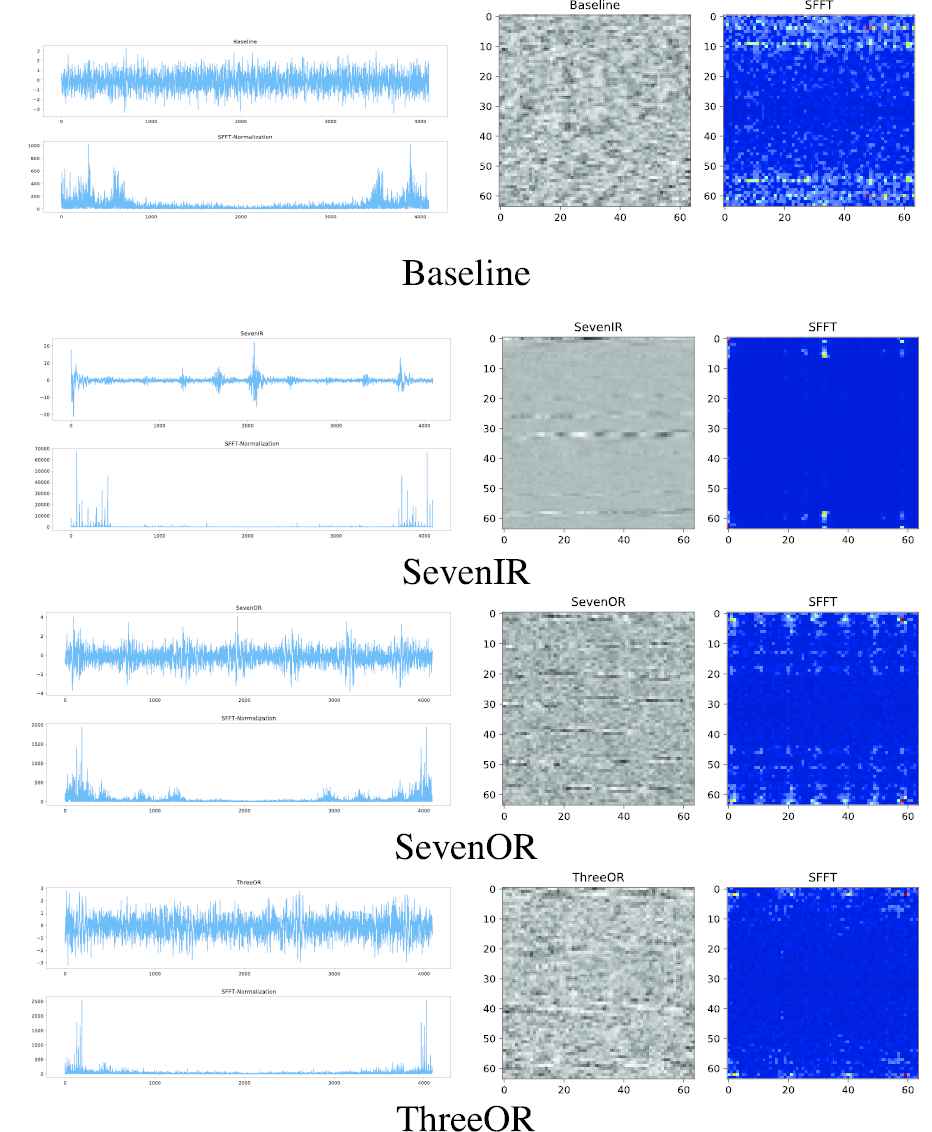
Signal and images of machinery failure prevention technology (MFPT) dataset.
3.2.2. Comparison results
CNN-T is compared with existing results from other different methods. From Table 7, it can be seen that an accuracy of 99.9% is the best result for other methods, whereas our CNN-T method can achieve an accuracy of 100% within ten running times. Especially, CNN using the time-frequency information of wavelet does not perform well because of its complex CNN structure that uses three repetitive CCP layers [9].
| Method | Average Accuracy | Number of Classes |
|---|---|---|
| CNN-T (W = 96) | 100 | 4 |
| CNN-T (W = 64) | 99.99 | 4 |
| CNN-Wavelet 96 × 96 [9] with CNN [27] | 99.9 | 3 |
| CNN- Wavelet 96 × 96 [9] | 99.9 | 3 |
| 1D-3 LAYER CNN [33] | 98.32 | 3 |
Comparison results of different methods with machinery failure prevention technology (MFPT) dataset (Pt = 0.8, %).
3.2.3. Sensitivity with samples and W
According to Ref. [32],
To investigate the effects of different parameters on the classification accuracy, some experiments with different W values (W = 32, 64, 96) and Pt values (Pt = 0.1, 0.5, 0.8) are conducted, and the results are given in Table 8.
| W | Pt | Min | Max | Mean | Std |
|---|---|---|---|---|---|
| 96 | 0.8 | 100.00 | 100.00 | 100.00 | 0.00 |
| 96 | 0.5 | 100.00 | 100.00 | 100.00 | 0.00 |
| 96 | 0.1 | 99.68 | 100.00 | 99.93 | 0.09 |
| 64 | 0.8 | 99.95 | 100.00 | 99.99 | 0.02 |
| 64 | 0.5 | 99.92 | 100.00 | 99.99 | 0.02 |
| 64 | 0.1 | 99.50 | 99.97 | 99.83 | 0.12 |
| 32 | 0.8 | 99.65 | 99.95 | 99.85 | 0.10 |
| 32 | 0.5 | 99.48 | 99.76 | 99.63 | 0.09 |
| 32 | 0.1 | 97.56 | 98.43 | 97.96 | 0.29 |
Classification accuracies with different parameters (%).
As can be seen from Table 8, the classification accuracy with W = 32 cannot achieve 100% because of W < 56.66, and the maximum accuracy can achieve 100% when W = 64 and Pt = 0.5 or 0.8. With the increase of W and Pt, our method has more chance to achieve an accuracy of 100%. Furthermore, the results are not sensitive to W and Pt except the situation of an accuracy of 100%.
3.3. Self-priming Centrifugal Pump Dataset
In the test bed, an acceleration sensor is fixed on a specific pedestal, with a revolving speed of 2900 rpm. The sampling frequency is 10239 Hz. Five categories of data are recorded, and 10000 data samples shown in Table 9 are randomly extracted from the raw data file.
| Type of Fault | Number of Samples |
|---|---|
| Normal | 2000 |
| Roller wearing | 2000 |
| Impeller wearing | 2000 |
| Outer race | 2000 |
| Inner race | 2000 |
Samples of self-priming centrifugal pump (SPCP) dataset.
In comparison with CNN-VibrationImage [7] and SURF-based PNN [17], our proposed method is the most efficient and can achieve an accuracy of 100%, as shown in Table 10.
3.4. Axial Piston Hydraulic Pump Dataset
An accelerograph is installed on the end face of the pump, with a revolving speed of 5280 rpm. The sampling frequency is 1 kHz. There are three categories of signals, and about 4000 data samples shown in Table 11 are randomly extracted from the raw data file. For ten times of independent run with Pt = 0.8 and W = 16 or 20, as shown in Table 12, our method can achieve the same classification accuracies as CNN-VibrationImage does [7].
| Type of Fault | Number of Samples |
|---|---|
| Normal | 921 |
| Valve plate wearing | 1228 |
| Piston shoes and swashplate wearing | 1842 |
Samples of axial piston hydraulic pump (APHP) dataset.
3.5. Probability to Achieve 100% Accuracy
In this study, four datasets have been used to verify the efficiency of our proposed CNN-T method. According to the above experimental results, the statistical probabilities to achieve 100% accuracy within ten times of independent run are given in Table 13.
| Dataset | W | Pt | P100 |
|---|---|---|---|
| CWRU | 96 | 0.8 | 1 |
| CWRU | 96 | 0.5 | 0.7 |
| CWRU | 64 | 0.8 | 0.5 |
| MFPT | 96 | 0.8 | 1 |
| MFPT | 96 | 0.5 | 1 |
| MFPT | 96 | 0.1 | 0.3 |
| MFPT | 64 | 0.8 | 0.9 |
| MFPT | 64 | 0.5 | 0.7 |
| SPCP | 64 | 0.8 | 1 |
| APHP | 20 | 0.8 | 1 |
| APHP | 16 | 0.8 | 0.9 |
Statistical probability for different datasets to achieve an accuracy of 100%.
It can be found that larger W and Pt values have higher probability to achieve 100% classification accuracy and that W is the dominated factor. For example, when CWRU and MFPT datasets are used, W = 96 has a high chance to achieve 100% accuracy. Figure 8 shows the t-SNE visualization result of CNN layer “F5” output of CWRU dataset. As can be seen, with the increase of W, different fault data can be easily distinguished from each other. In addition, lower Pt means a small number of samples, which will lead to less probability to reach 100% accuracy and perform less efficiently. For example, Pt = 0.5 has only 70% probability while Pt = 0.8 has 100% probability when CWRU dataset with W = 96 is used.
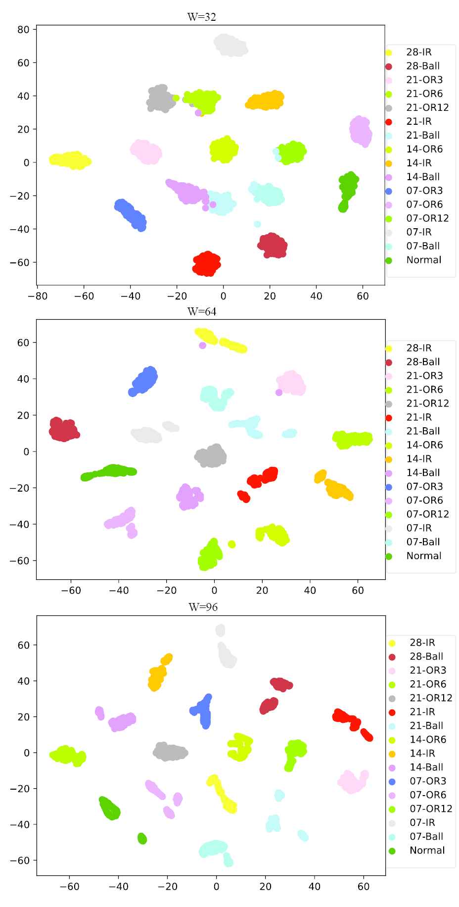
t-SNE visualization of Case Western Reserve University (CWRU) dataset for test (Pt = 0.8).
4. CONCLUSIONS
In this study, we propose an efficient universal CNN with tunable input-size W*W for bearing fault diagnosis (CNN-T). With the guidance of theoretic analysis about the relationship between the characteristic vibration frequencies and the window size of STFT, the low bound of W that decides the input size of the matrix fed to CNN can be determined readily. With the increase of W, robust results can be obtained by CNN-T, but too large W may cause the performance degradation due to longer running time.
The proposed method has been tested with four different datasets. After ten times of independent run, all classification accuracies for these four datasets can achieve 100%. Moreover, our proposed method is suitable for different datasets without any change of CNN structure, and the only thing is to adjust the parameter W. Hence, the CNN-T method is more general and flexible.
In the future, datasets with more classes of faults will be tested to further verify the performance of CNN-T, and great efforts are required to find unknown faults and fault severity [39]. Furthermore, transfer learning between different datasets is also a popular topic to improve the adaptability of deep learning [40].
CONFLICTS OF INTEREST
No potential conflict of interest was reported by the author(s).
AUTHORS' CONTRIBUTIONS
Jungan Chen: Conceptualization, Methodology, Software, Writing; Jean Jiang: Project Administration, Resources, Investigation; Xinnian Guo: Data Curation, Visualization, Software, Validation; Lizhe Tan: Supervision, Reviewing and Editing.
ACKNOWLEDGMENTS
This work was supported in part by National Natural Science Foundation of China (No. 61502423), Zhejiang Provincial Natural Science Foundation (No. LY16G020012), and Zhejiang Province Public Welfare Technology Application Research Projects (Nos. LGF19F010002, LGN20F010001, and LGF20F010004, LGG21F030014: The Research on Cold-Start Fault Diagnosis Method Based on Immune Algorithm and Deep Learning).
REFERENCES
Cite this article
TY  - JOUR
AU  - Jungan Chen
AU  - Jean Jiang
AU  - Xinnian Guo
AU  - Lizhe Tan
PY  - 2021
DA  - 2021/01/20
TI  - An Efficient CNN with Tunable Input-Size for Bearing Fault Diagnosis
JO  - International Journal of Computational Intelligence Systems
SP  - 625
EP  - 634
VL  - 14
IS  - 1
SN  - 1875-6883
UR  - https://doi.org/10.2991/ijcis.d.210113.001
DO  - 10.2991/ijcis.d.210113.001
ID  - Chen2021
ER  -