
Forecasting Teleconsultation Demand with an Ensemble Attention-Based Bidirectional Long Short-Term Memory Model
 , Jinlin Li1, *,
 - DOI
- 10.2991/ijcis.d.210203.004How to use a DOI?
- Keywords
- Teleconsultation; Demand forecast; Holiday effect; Attention mechanism; Deep learning ensemble; Bidirectional long short-term memory (BILSTM)
- Abstract
Accurate demand forecast can help improve teleconsultation efficiency. But teleconsultation demand forecast has not been reported in existing literature. For this purpose, the study proposes a novel model based on deep learning algorithm for daily teleconsultation demand forecast to fill in the research gap. Because of the significant effect of holidays on teleconsultation demand, holiday-related variables, and specific prediction technologies were selected to treat it. The technologies attention mechanism and bidirectional long short-term memory (BILSTM) were used to construct a novel forecasting methodology, i.e., ensemble attention-based BILSTM (EA-BILSTM), for the accurate forecasts. Based on actual teleconsultation data, the effectiveness of variable selection is verified by importing different inputs into models, and the superiority of EA-BILSTM is verified by comparison with nine benchmark models. Empirical results show that importing selected variables can lead to better forecasts and EA-BILSTM model can get lowest forecasting errors on two sub-datasets. This indicates that the proposed forecasting model is a high potential approach for teleconsultation demand prediction in the influence of sparse trait, like holiday effects.
- Copyright
- © 2021 The Authors. Published by Atlantis Press B.V.
- Open Access
- This is an open access article distributed under the CC BY-NC 4.0 license (http://creativecommons.org/licenses/by-nc/4.0/).
1. INTRODUCTION
To omit geographical and functional distance, advanced information and communication technologies (ICTs) are used in telemedicine healthcare services. Telemedicine can often be divided into three modes: teleconsultation, remote monitoring, and remotely supervised treatment or training [1]. Teleconsultations are remote meetings between two or more geographically separated health providers or between health providers and patients for diagnosis or treatment of diseases [2]. At the present stage in National Telemedicine Center of China (NTCC), teleconsultation is a service that doctors at primary hospitals ask for the help of the doctors at class-A tertiary hospitals to diagnose or treat difficult miscellaneous diseases [3]. By this way, teleconsultation can sink high-quality medical resources to underdeveloped areas to alleviate the shortage and uneven distribution of medical resources in China. Because of the function, teleconsultation played an important role in the battle against COVID-19 in the beginning of 2020.
In recent years, more and more hospitals are networked with NTCC, so the demand of teleconsultation has increased gradually. To increase the efficiency of teleconsultation, rational arrangements of triage coordinators and consultation rooms are crucial. To realize this objective, accurate demand forecast can be of help by avoiding unbalanced supply and demand. However, teleconsultation demand forecast hasn't been reported in existing literatures. Previous studies of telemedicine focus on the use introduction [4,5], effect evaluation [6–8], technology development [9], and some operations and management studies. In the operations and management literature, resource allocation [3], appointment and scheduling [10], face-to-face visit prediction [11], blood pressure prediction [12], chronic wound tissue prediction [13], framework development [14], the need survey of healthcare providers [15], and patient preferences [16] are involved.
In previous studies, there is no forecasting model of daily teleconsultation demand. For this purpose, the study tries to develop the forecasting model to fill in the research gap. To build an effective model with high performance, the trait of teleconsultation demand time series data was analyzed firstly. In teleconsultation, the demand is significantly affected by holidays. Specifically, the demand before holidays decreases (pre-effect), and the demand on holiday can decrease to zero. Besides, the demand after holidays is less than the ordinary working days. In all, the holiday effect on teleconsultation demand does not only affect whole holidays but also affect working days near to holidays. In terms of this holiday effect, some related variables were selected as the part of model input, and the attention mechanism and didirectional long short-term memory (BILSTM) were selected to build the forecasting model. For improvement, considering the pre-effect of holidays on teleconsultation demand, a deep learning ensemble framework was proposed to use future information and avoid useless information. Based on this framework, an ensemble attention-based BILSTIM (EA-BILSTM) model was proposed for final prediction purpose.
The main contributions of this paper are described as follows:
This study is the first work to build the forecast model of daily teleconsultation demand for optimizing teleconsultation resources.
This study increases the prediction accuracy of daily teleconsultation demand by elaborating treatment to holiday effect. The holiday effect is tackled by variable selection and model construction.
Deep learning algorithm, attention mechanism, and ensemble method are used to construct a novel forecasting model for teleconsultation demand. This study is also the first work to use those techniques to handle with the holiday effect in demand forecasts.
To illustrate the effectiveness of variable selection and superiority of the proposed model, empirical studies are conducted on actual teleconsultation demand data. Also, the influence of data quantity on the demand forecast is analyzed.
The rest of the paper is organized as follows: Section 2 gives a review of the literature related to demand forecast and holiday effect. Section 3 introduces the ensemble methodology. Section 4 introduces the datasets and experimental designs. Section 5 presents the experimental results and Section 6 gives the discussions. Finally, Section 7 concludes the paper.
2. LITERATURE REVIEW
Demand forecast has been studied in many areas, such as energy [17,18], tourism [19,20], supply chain [21], traffic [22,23], and healthcare [24–30]. In the area of healthcare, most of the demand forecast focused on emergency department (ED). For example, patient visits to ED forecast studies before 2009 were reviewed in [26]. In the identified 9 studies, most of the models used to forecast the number of the patient were either linear regression models including calendar variables or time series models. The study in [27] demonstrated autoregressive integrated moving average (ARIMA) can be used to forecast, at least in the short term, demand for emergency services in a hospital ED. For monthly ED demand forecast, multivariate vector-ARIMA (VARIMA) models provided a more precise and accurate forecast than the ARIMA and Winters' method [28]. For improving forecasts in [29], patients were classified before the ED patients flow were forecasted in the long term and the short term. And for short- and long-term forecast of ED attendances, modified heuristics based on a fuzzy time series model was developed in [30], which was proved to outperform ARIMA and neural network (NN) model.
Demand forecast is more difficult than some time series prediction because of the influence of holidays on the demand change. The holiday effect in healthcare has been identified [31,32]. Teleconsultation demand is also affected by the holidays. Some staffs, like triage nurses and device administrator in NTCC are day off in holidays. Therefore, when holidays are coming, applications for teleconsultation will decrease.
In previous studies, when holiday effect existed, a number of methods were proposed to improve prediction performance. These methods can be divided into two categories, input treatment and model development. To handle holiday effect from input perspective, holidays were seen as an emergency event in [33]. The fluctuation coefficient of emergency event got by trend extrapolation was used to forecast the tourist demand, contributing higher forecasting accuracy. In a multi-stage of the input feature combination in [34], the identified optimal combination of the input features and their appropriate coding can improve the accuracy of passenger demand forecast, not only for the forecasting results on weekdays and weekends, but also for them on national holidays. In the traffic flow data, discrete Fourier transform was used to extract the common trend and support vector regression (SVR) was used to forecast the residual series [23]. Because of the hybrid approach, higher accuracy of traffic demand forecast during the holidays was achieved.
To handle holiday effect from model perspective, high-performance models were proposed by researchers. In [35], a hybrid model, combining SVR model with the adaptive genetic algorithm (GA) and the seasonal index adjustment, was proposed to forecast holiday daily tourist demand. In an attempt to forecast holiday passenger flow more accurately, a modified least squares support vector machine (LSSVM) was proposed in [36]. In this method, an improved particle-swarm optimization (IPSO) algorithm was used to optimize parameters of LSSVM and the pruning algorithm was used to achieve sparseness in the LSSVM solution. The results show that the modified LSSVM model was an effective forecasting approach with higher accuracy than other alternative models. To seize the weekly periodicity and nonlinearity characteristics of short-term ridership in practical application, a combined SVM online model was proposed in [37]. This method combined a support vector machine overall online model (SVMOOL) and a support vector machine partial online model (SVMPOL). The SVMOOL was inserted the weekly periodic characteristics and trained the updated data day by day, and the SVMPOL was inserted the nonlinear characteristics and trains the updated data of the predicted day by time interval. The experimental results demonstrated that the proposed SVM-based online model outperformed the seasonal ARIMA, back-propagation neural network (BPNN), and SVM. In [22], a convolutional neural network (CNN)-based multi-feature forecasting model (MF-CNN) was proposed, which collectively forecasts network-scale traffic flow with multiple spatiotemporal features and external factors.
From the literature review, the holiday effect is not an easy problem to tackle in time series forecasting. On the one hand, considering the holiday effect is lasting for a period of time, how to build and select the holiday-related variables is a state of art. On the other hand, the holidays are sparse distributed, and the date of some Chinese traditional holidays are not fixed. The sparseness and variability require the built model has powerful learning ability to learn the holiday influence. For traditional time series techniques and machine learning methods, the sparseness and variability of holiday effect make them cannot achieve satisfactory forecasting results. Thus, a flexible technique, with long memory on learning results and more attention to specific variables, is more suitable to deal with the sparse distributed and date-changed holiday effect. Among techniques, deep learning method with attention mechanism can be used to construct such a model with this powerful learning capability.
3. METHODOLOGY
To obtain better forecasts for teleconsultation demand in this study, deep learning algorithm, attention mechanism, and ensemble method are combined to deal with the holiday effect. The deep learning algorithm and attention mechanism are introduced in Section 3.1. The ensemble framework is introduced in Section 3.2. And based on the framework, a novel EA-BILSTM model is proposed for teleconsultation demand forecast in Section 3.3.
3.1. Deep Learning Algorithm and Attention Mechanism
In this section, a typical deep learning method named long short-term memory (LSTM) is introduced, which has advanced gate unites, namely input gate, output gate, and forget gate [38]. The input gate decides what new information can be stored in the cell state; the output gate decides what information can be output based on the cell state; and the forget gate can decide what information will be thrown away from the cell state. These gates units make LSTM suitable for processing and predicting events with very long intervals and delays in time series. Despite of this advantage, LSTM is only able to make use of previous information. In order to overcome this shortcoming, the bidirectional recurrent neural network (BRNN) was introduced by Schuster and Paliwal [39]. This kind of architecture could be trained in both time directions simultaneously, with separate hidden layers. Considering the pre-effect of holiday on teleconsultation demand, the BILSTM may improve the prediction performance. Furthermore, attention mechanism can improve forecasts by readjustment of weights on variables [40]. Attention mechanism has been widely used in natural language processing (NLP), showing outstanding performance [41,42]. And it is gradually applied in time series forecast, showing great potentiality [43].
3.2. The Proposed Attention-Based Deep Learning Ensemble Model
Under the background of significant holiday effect on teleconsultation demand, a deep learning ensemble framework is proposed to use as much useful information as possible for forecast improvement. Normally, forecasting models use history data to predict the future state. However, some information at the forecasted time or after the forecasted time are available, like the holiday information arranged by the government in several months advance. Due to the significant pre-effect of holidays on teleconsultation demand, introducing future holiday data into models can improve forecasts greatly. To use all available and useful information, the attention-based deep learning ensemble model is proposed and shown in Figure 1. In this ensemble model, a typical RNN, like LSTM or BILSTM, is used as the single predictor. In the proposed methodology, there are three main steps, which are elaborated below.
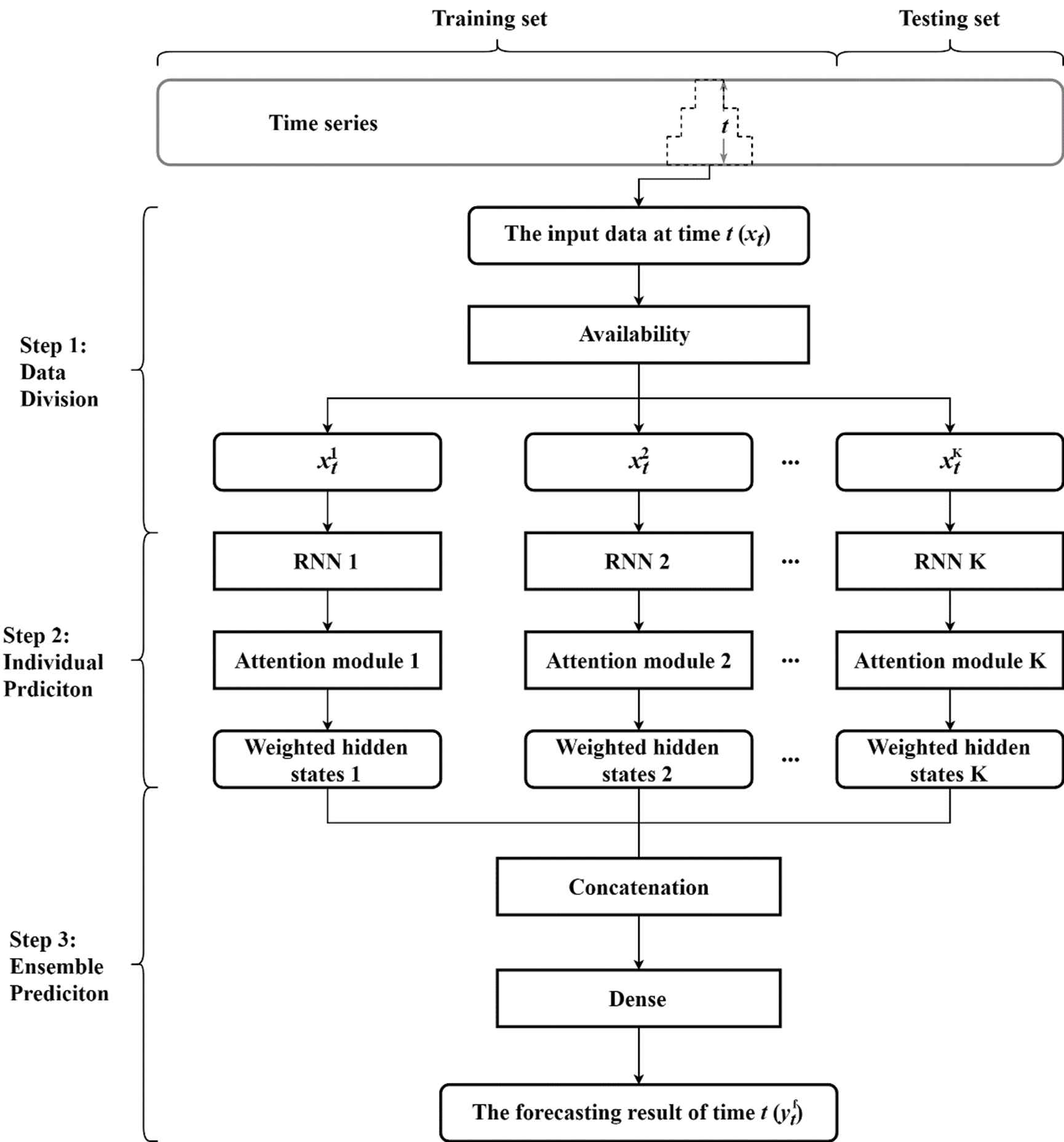
The generic framework of the proposed deep learning ensemble model.
Step 1: Data Divisions
In the beginning, the input data matrix at time t may be in irregular shape because of the different data availability. Data can have different availability at time t because of the different frequencies in data collection or the unknown future information of some variables. According to the different availability, the input data can be divided into different inputting sub-matrices. Variables contained same availability are divided into one group as one input. Variables can be repeatedly used. High available variables can be included in low available variable-groups. Figure 2 gives the example of data division when the data have two availability.
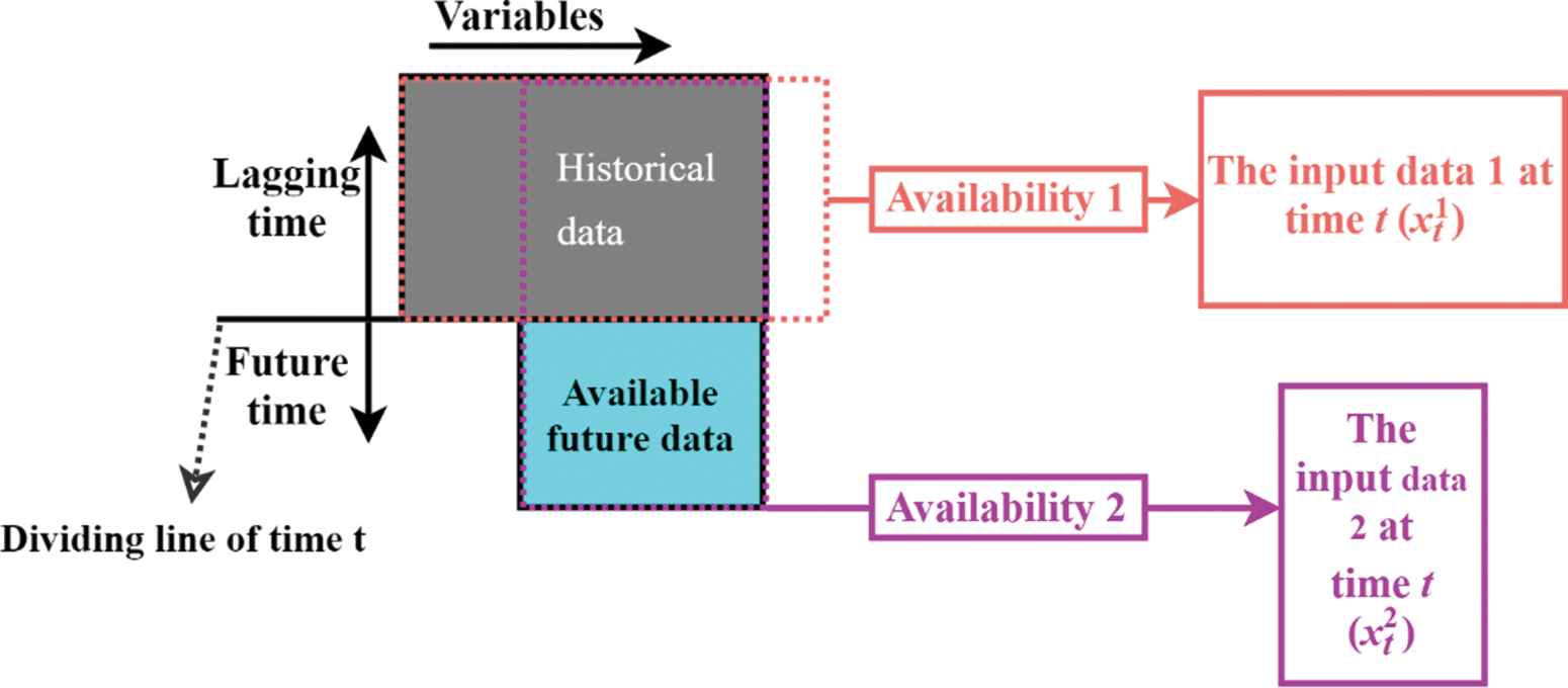
The example of input data division for data with two availability.
Step 2: Individual Prediction
Each data sub-matrix is input into a RNN with an attention module. Because of the capability of the attention module, the hidden states of RNN are weighted and they are seen as the results of the individual prediction.
Step 3: Ensemble Prediction
Attention-based RNN outputs the weighted hidden states in Step 2. In Step 3, all weighted hidden states are concatenated together as the input of the dense layer. This layer is a regular densely-connected NNs layer. And in this study, the activation of it is the sigmoid. Finally, the dense outputs the final ensemble prediction result of time t.
3.3. The Proposed EA-BILSTM Model
Given the pre-effect of holidays on teleconsultation demand, this study applied attention-based BILSTM to build the forecasting model for teleconsultation demand. Besides, for better use of the future information, an EA-BILSTM model is proposed for the final teleconsultation demand prediction based on the ensemble framework. The proposed EA-BILSTM model in this paper is shown in Figure 3.
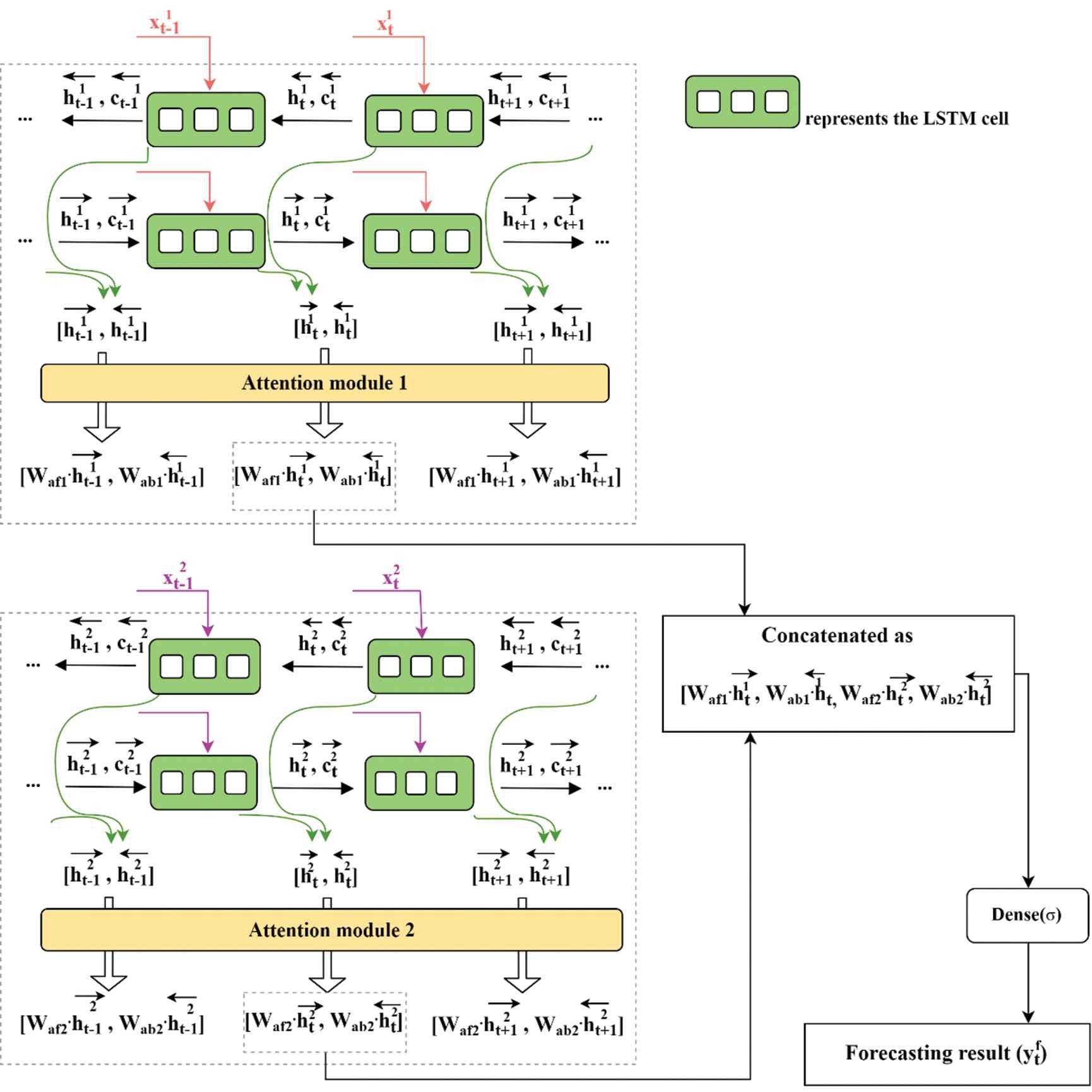
The proposed ensemble attention-based bidirectional long short-term memory (EA-BILSTM) model for teleconsultation demand forecast.
There are two available data on the predicted time t, available historical demand data and holiday data, and available future holiday data. Therefore, the input data at time t can be divided into two sub-matrices. Then, these two sub-matrices are respectively introduced into the BILSTM and attention module to obtain individual predictions. Individual prediction results
To get ensemble predictions, the individual results are aggregated as the input of the dense layer. The final prediction
4. DATA DESCRIPTION AND EXPERIMENTAL DESIGN
To testify the effectiveness of variable selection and the superiority of the proposed EA-BILSTM model, the actual teleconsultation demand data are used as the sample data. And other forecasting techniques (including traditional models, machine learning models, and single deep learning models) are introduced for comparison. Section 4.1 describes the data and Section 4.2 presents the experimental design.
4.1. Dataset
The dataset in this study is the application records of teleconsultation collected in NTCC [3]. The dataset consists of the number of the application from January 1, 2018, to November 30, 2019, with a total of 668 observations. That is, in these 699 days, the records of 31 days were missing.
Besides the missing data, the holiday effect is significant in teleconsultation demand. Taking the data from January 1, 2018, to April 30, 2018, as example, the demand changes with date are shown in Figure 4. The holidays have two main effect on the demand. On the one hand, the demands in the holidays are much less than the ordinary working days. And the demands before and after holidays are also less than ordinary working days. On the other hand, the holidays bring variations on the weekly pattern of teleconsultation demand. In Figure 4, it can be also observed that some missing data are caused by the holidays. Before missing data treatment, the variables relating to the holiday are selected.
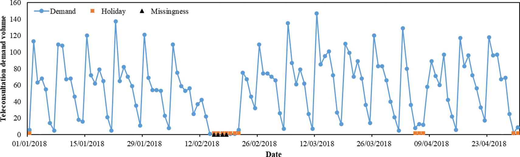
The changes of teleconsultation demand volume with date.
Because sample volume affects forecasting results [44], therefore, three sub-datasets with different sample volumes are used in the experiments of this study. They are 365-day dataset (January 1, 2018, to December 31, 2018), 548-day dataset (January 1, 2018, to July 2, 2019), and 699-day dataset (January 1, 2018, to December 30, 2019). In the 365-day dataset and 548-day dataset, 70% observations are used as their training datasets, and remaining 30% observations are used as the testing datasets. In 699-day dataset, 60% observations are used as the training dataset, and remainder 40% observations are used as the testing dataset. The testing set of 699-day dataset accounts for 40% to make the testing dataset include more holidays for the learning effect test of holiday influence.
4.2. Experimental Designs
The experiment designs are presented in this section, in terms of variable selection, missing data treatment, evaluation criteria, benchmark models, and model inputs.
4.2.1. Selection of holiday-related variables
To introduce the holiday information into forecasting models, holiday-related variables are selected. First of all, week and holiday are the commonly used variables, and they are included in the selection. In addition, considering the spillover effect of holidays on teleconsultation demand, other eight variables are adopted, including the length of holiday, the first, second, third day before and after the holiday, and weekends shifted to working days. Variables are selected by significance of coefficients in the constructed linear regression equation, as shown in Table 1. The coefficients of seven variables were significant with the 5% significance level. So those seven variables were selected as the holiday-related part of the input data. Furthermore, the significance of the second and first day before the holiday and the first day after the holiday proves that the holidays have spillover effect on teleconsultation demand.
| Variables | Week | Holiday | Length of Holiday | The Third |
The Second |
The First |
The First |
The Second |
The Third |
Adjusted as Working Day |
|---|---|---|---|---|---|---|---|---|---|---|
| Day Before the Holiday | Day After the Holiday | |||||||||
| Values | 1–7 | 0, 1 | 3, 4, 7 | 0, 1 | 0, 1 | 0, 1 | 0, 1 | 0, 1 | 0, 1 | 0, 1 |
| Coefficients | −13.19 | −27.88 | −3.55 | −0.37 | −13.39 | −33.47 | 22.11 | 3.21 | 3.61 | 17.21 |
| Significance* | <0.01 | <0.01 | <0.01 | 0.943 | 0.013 | <0.01 | <0.01 | 0.524 | 0.475 | <0.01 |
is the significance of coefficients in constructed linear regression equation.
Selection of holiday-related variables.
4.2.2. Treatment of missing data
According to the missing mechanism and missing pattern [45], three kinds of missing data are treated in teleconsultation demand data. And they are discrete missingness at random (DMAR), continuous missingness at random (CMAR), and missing completely at random (MCAR). For these different missing data, feature-driven method and LSTM model are used to treat the missingness, as shown in Table 2. To evaluate the effect of missing data treatments, two evaluation criteria, root mean square error (RMSE), and mean absolute error (MAE) of LSTM are utilized. The treatment with the best forecasting performance of LSTM is selected as the finally applied missingness treatment for later experiments. According to the values of RMSE and MAE, 0 imputation for DMAR and CMAR, and LSTM imputation for MCAR are the best missingness treatment methods. The next models will be built on the dataset treated by these imputation methods.
| Missing Data Treatment |
LSTM Performance |
|||
|---|---|---|---|---|
| DMAR | CMAR | MCAR | RMSE | MAE |
| Deletion | Deletion | LSTM imputation | 14.37 | 11.57 |
| 0 imputation | 0 imputation | LSTM imputation | 14.27 | 11.33 |
| Deletion | 0 imputation | LSTM imputation | 15.76 | 12.55 |
| 0 imputation | Deletion | LSTM imputation | 14.69 | 11.45 |
Note: The underlines are the best performance of each column.
LSTM, long short-term memory; DMAR, discrete missingness at random; CMAR, continuous missingness at random; MCAR, missing completely at random; RMSE, root mean square error; MAE, mean absolute error.
Missing data treatment methods and results.
4.2.3. Evaluation criteria and statistic test
To assess forecasting accuracy, two criteria are applied and they are the root mean squared error (RMSE) and the MAE:
To provide statistical evidence of the forecasting ability of the proposed model, the Diebold-Mariano (DM) test is introduced on MAE to identify the significant forecasting differences in models. DM test determines whether there is a significant difference between two prediction models under the assumption that the performance error between them is 0 (the null hypothesis). Under this assumption, DM follows a standard normal distribution. Thus, there is a significant difference between the prediction models if
4.2.4. Benchmark models
To illustrate the superiority of the proposed EA-BILSTM, nine models are applied as the benchmarks. The benchmarks include the traditional econometric model such as ARIMA model, four machine learning models, K nearest neighbor (KNN), SVR, NNs, extreme learning machine (ELM), and four deep learning models, LSTM, BILSTM, attention-based LSTM (A-LSTM), attention-based BILSTM (A-BILSTM). These four deep learning models are respectively used to build their ensemble models, denoted as E-LSTM, E-BILSTM, EA-LSTM, EA-BILSTM.
4.2.5. Inputs of models
To prove the effect of holiday-related variables and future available information, different inputs are constructed for models. Firstly, the historical demand data is the basic input variable. Univariate ARIMA model only uses historical demand information to predict the future demand. For building ARIMA model, characteristic analysis of time series is necessary. First, the nonstationarity of the teleconsultation demand is clearly visible due to the weekly periodic pattern in Figure 4. To further test the nonstationarity of the time series, unit root test is applied. It supposes the time series has a unit root (null hypothesis) and the time series is nonstationary. The test result shows teleconsultation demand data is nonstationary (p = 0.243). Because of the nonstationarity, a first difference with 7 lags is applied to the demand series to make it stationary. Second, periodicity can also influence the parameters of ARIMA and the length of the historical data in the inputs of other multivariate models. According to the plots in Figure 3 and the autocorrelation and partial autocorrelation analysis, teleconsultation data had the 7-day cycle. Thus, the maximum time lag in ARIMA is set to 7 and the length of historical data in inputs is set to 7.
For other multivariate models, input dimensions can include different numbers of variables. One group of variables are the historical demand volume and the two commonly used date variables (week and holiday). Another group of variables are the historical demand volume and seven selected variables in Section 4.2.1. Those two groups of variables only use historical information. However, some information at the forecasted time or after the forecasted time are available, like the holiday information. Therefore, the date information of the T day (the forecasted time) and
| Input |
|||||||
|---|---|---|---|---|---|---|---|
| Model | Size |
Variables |
|||||
| Length (Days) | Number of Variables | Demand | Week | Holiday | Other Five Holiday-Related Variablesa | ||
| Single model 1 | Input 1 | 7 ( |
3 | √ | √ | √ | |
| Single model 2 | Input 2 | 7 ( |
8 | √ | √ | √ | √ |
| Single model 3 | Input 3c | 9 ( |
8 | √ | √ | √ | √ |
| Ensemble model | Input 2 | 7 ( |
8 | √ | √ | √ | √ |
| Input 4 | 9 ( |
7 | √ | √ | √ | ||
Other five holiday-related variables include length of holiday, the second day before holiday, the day before holiday, the day after holiday, adjusted as working day.
The demand on day T was forecasted.
The demand of T and
Different inputs of forecasting models.
5. EMPIRICAL RESULTS
Due to the significant pre-effect of holidays on teleconsultation demand, holiday-related variables are selected and EA-BILSTM is constructed for the accurate demand forecast. To verify the effectiveness of the selected variables and the proposed model, actual teleconsultation demand data collected in NTCC are used as the sample data. In the empirical studies, traditional ARIMA model, machine learning models, single deep learning models are applied as benchmarks. In the two groups of models (machine learning models and single deep learning models), Model-1 represents input-1 is introduced into the corresponding model, Model-2 represents input-2 is introduced into the corresponding model, and Model-3 represents input-3 is introduced into the corresponding model. To compare the performance of models, RMSE and MAE are measured as shown in Table 4.
| Model | 365-Day Dataset |
548-Day Dataset |
699-Day Dataset |
|||
|---|---|---|---|---|---|---|
| Performance |
Performance |
Performance |
||||
| RMSE | MAE | RMSE | MAE | RMSE | MAE | |
| ARIMA | 19.47 | 12.07 | 15.95 | 11.66 | 15.72 | 10.83 |
| KNN-1 | 20.95 | 12.89 | 19.87 | 13.85 | 16.14 | 11.57 |
| SVR-1 | 18.52 | 12.77 | 18.83 | 13.78 | 14.82 | 11.42 |
| NN-1 | 18.67 | 12.75 | 20.41 | 14.87 | 20.17 | 14.25 |
| ELM-1 | 19.21 | 12.74 | 20.66 | 14.36 | 15.91 | 11.19 |
| KNN-2 | 19.21 | 13.07 | 19.78 | 13.98 | 16.25 | 11.90 |
| SVR-2 | 18.18 | 13.30 | 17.44 | 13.68 | 15.37 | 12.26 |
| NN-2 | 19.58 | 12.45 | 19.13 | 13.74 | 16.02 | 11.26 |
| ELM-2 | 23.80 | 14.71 | 21.72 | 15.01 | 19.78 | 13.04 |
| KNN-3 | 15.50 | 11.30 | 16.00 | 11.77 | 14.22 | 10.37 |
| SVR-3 | 15.77 | 12.49 | 15.99 | 12.77 | 14.42 | 11.77 |
| NN-3 | 14.67 | 10.52 | 16.00 | 11.82 | 14.32 | 10.75 |
| ELM-3 | 18.57 | 13.09 | 17.53 | 13.05 | 17.63 | 11.96 |
| LSTM-1 | 13.62 | 10.23 | 19.08 | 13.16 | 15.95 | 11.07 |
| BILSTM-1 | 13.82 | 10.27 | 18.13 | 13.01 | 15.70 | 10.91 |
| A-LSTM-1 | 14.70 | 10.20 | 19.27 | 12.88 | 15.83 | 10.88 |
| A-BILSTM-1 | 14.26 | 9.51 | 16.67 | 11.28 | 17.50 | 10.87 |
| LSTM-2 | 17.77 | 12.12 | 18.02 | 12.31 | 14.33 | 10.24 |
| BILSTM-2 | 15.01 | 10.48 | 16.46 | 12.02 | 14.97 | 10.07 |
| A-LSTM-2 | 14.40 | 9.99 | 17.02 | 11.53 | 14.32 | 10.02 |
| A-BILSTM-2 | 13.83 | 9.10 | 15.36 | 11.12 | 13.55 | 9.72 |
| LSTM-3 | 14.55 | 10.34 | 15.36 | 11.09 | 14.07 | 10.65 |
| BILSTM-3 | 14.93 | 10.36 | 15.69 | 11.57 | 13.66 | 10.08 |
| A-LSTM-3 | 15.42 | 9.93 | 15.96 | 11.34 | 13.97 | 10.00 |
| A-BILSTM-3 | 14.34 | 9.60 | 15.47 | 11.12 | 13.98 | 9.87 |
| E-LSTM | 15.95 | 10.74 | 15.98 | 11.83 | 13.40 | 9.82 |
| E-BILSTM | 14.32 | 9.71 | 15.51 | 11.38 | 13.67 | 9.93 |
| EA-LSTM | 14.94 | 10.06 | 16.28 | 11.46 | 13.86 | 9.86 |
| EA-BILSTM | 14.85 | 9.81 | 15.06 | 10.60 | 13.02 | 9.45 |
Notes: The bolds are the best performance in each group of models (machine learning models, single deep learning models, and ensemble deep learning models). The underlines are the best performance of each column.
LSTM, long short-term memory; RMSE, root mean square error; MAE, mean absolute error; ARIMA, autoregressive integrated moving average; KNN, K nearest neighbor; SVR, support vector regression; NN, neural network; ELM, extreme learning machine; BILSTM, bidirectional long short-term memory; A-LSTM, attention-based LSTM; A-BILSTM, attention-based BILSTM.
Prediction performance on three datasets.
Forecast performance changes with the different models, inputs, and datasets. From model perspective, there are three main important conclusions. First, ARIMA can outperform some single models but can't outperform ensemble models in term of the values of RMSE and MAE. For example, ARIMA has lower MAE than that of SVRs and ELMs, but it has higher MAE than EA-LSTMs and EA-BISLTMs. Second, all single deep learning models outperform the machine learning models. Because the best performance in machine learning models is inferior to that of single deep learning models. In the group of machine learning models, the lowest MAEs in three datasets are 10.52, 11.77, and 10.37. But in the group of single deep learning models, the lowest MAEs in three datasets are 9.10, 11.07, and 9.72. Third, the EA-BISLTM needs enough data quantity to ensure its outperformance. When data quantity increases to 548 and 699, EA-BILSTM obtained the lowest RMSE and MAE.
From input perspective, there are also three main important conclusions. First, introducing more information into the forecasting models can improve prediction performance. In machine learning models, the best performances on three datasets are achieved by introducing Input-3. Similarly, in single deep learning models, the best performances are achieved by introducing Input-2 and Input-3. Second, introducing useless information into deep learning models cannot improve forecasting performance. When Input-3 is introduced, some single deep learning models cannot obtain better performance. Third, introducing useful information and avoiding useless information into prediction models can improve forecasts. In particular, EA-BISLTM can obtain best performance on both 548-day dataset and 699-day dataset. From data perspective, complex structural model is more advantageous when data quantity is large enough for its training. For example, the EA-BISLTM model cannot obtain best performance on 365-day dataset but it can obtain best performance on 548-day dataset and 699-day dataset.
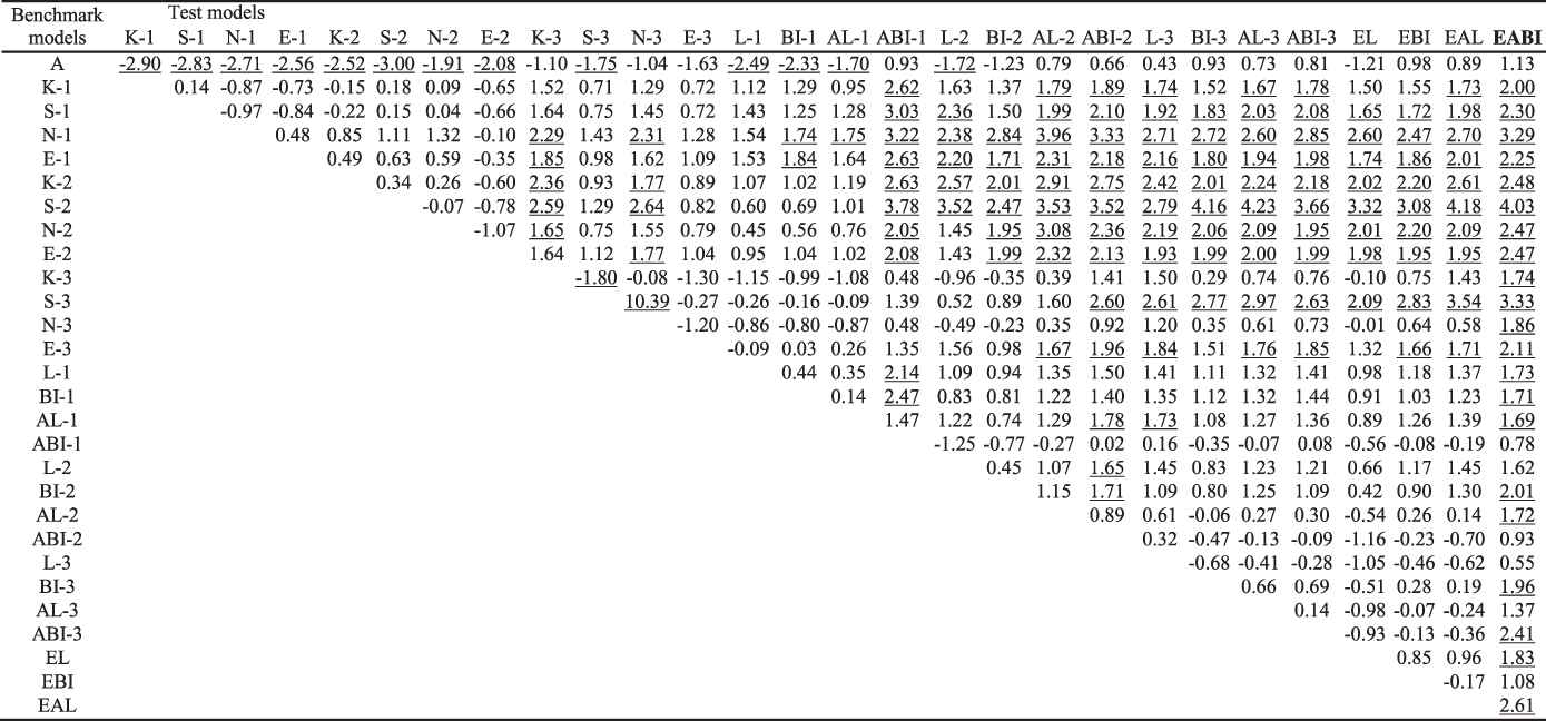
To identify the significance of the performance difference, DM test was applied on MAE. The DM test results are shown in Tables 5–7. In the test statistics, ±1.65 are used for the thresholds to identify the 0.1 significance level. Negative statistics mean the MAE of benchmark models are inferior to that of testing models, and benchmark models outperform testing models. Positive statistics mean test models outperform benchmark models.
 |
Notes: (1) Model abbreviations: A: ARIMA, K-1: KNN-1, S-1: SVR-1, N-1: NN-1, E-1: ELM-1, K-2: KNN-2, S-2: SVR-2, N-2: NN-2, E-2: ELM-2, K-3: KNN-3, S-3: SVR-3, N-3: NN-3, E-3: ELM-3, L-1: LSTM-1, BI-1: BILSTM-1, AL-1: A-LSTM-1, ABI-1: A-BILSTM-1, L-2: LSTM-2, BI-2: BILSTM-2, AL-2: A-LSTM-2, ABI-2: A-BILSTM-2, L-3: LSTM-3, BI-3: BILSTM-3, AL-3: A-LSTM-3, ABI-3: A-BILSTM-3, EL: ELSTM, EBI: E-BILSTM, EA-L: EALSTM, EABI: EA-BILSTM. (2) The underlines are out of range (-1.65, 1.65), meaning the MAE difference are significant. (3) The bold model gets the lowest MAE. (4) Table 6 and Table 7 have the same notes with Table 5.
DM test results of MAE for 365-day dataset.
 |
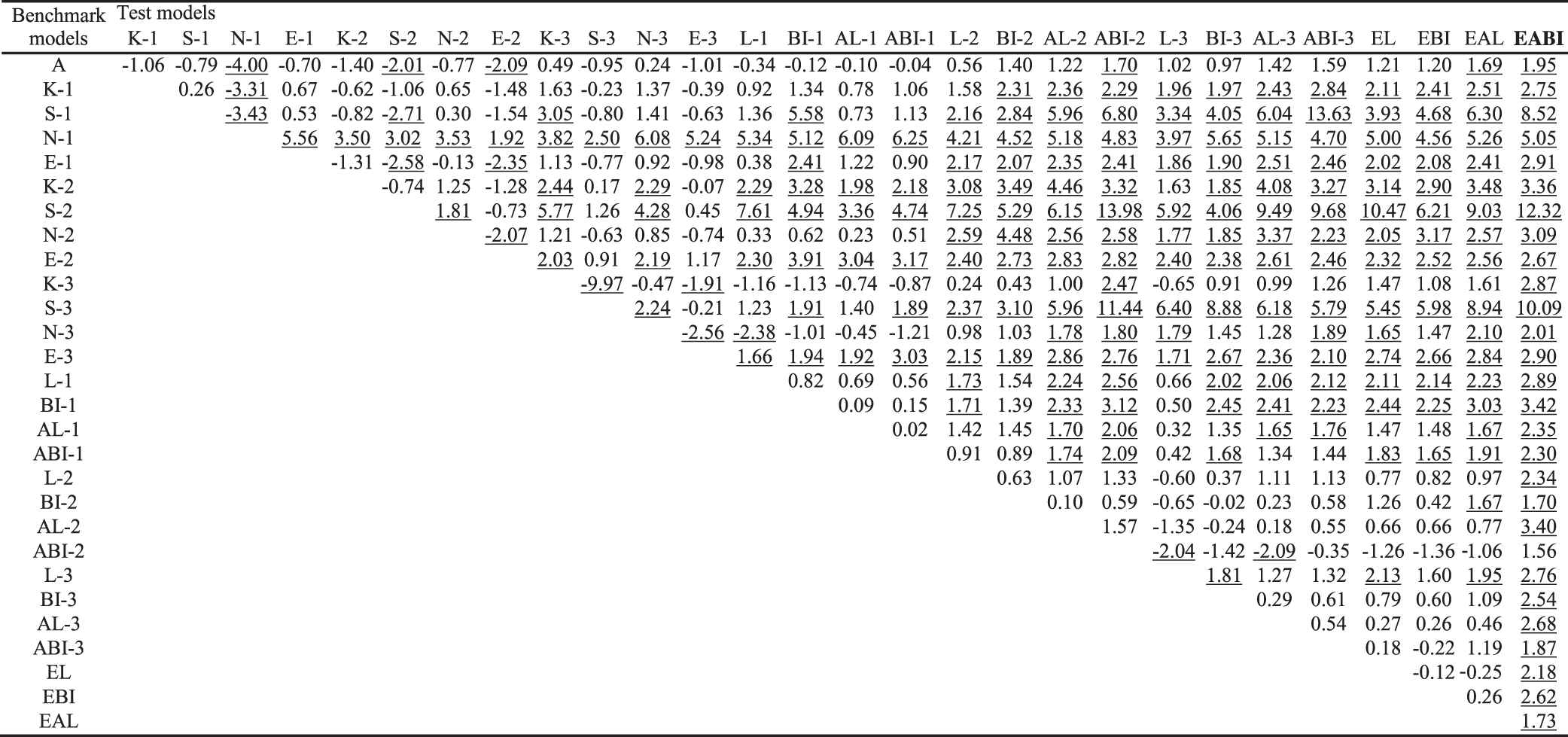
Notes: (1) Model abbreviations: A: ARIMA, K-1: KNN-1, S-1: SVR-1, N-1: NN-1, E-1: ELM-1, K-2: KNN-2, S-2: SVR-2, N-2: NN-2, E-2: ELM-2, K-3: KNN-3, S-3: SVR-3, N-3: NN-3, E-3: ELM-3, L-1: LSTM-1, BI-1: BILSTM-1, AL-1: A-LSTM-1, ABI-1: A-BILSTM-1, L-2: LSTM-2, BI-2: BILSTM-2, AL-2: A-LSTM-2, ABI-2: A-BILSTM-2, L-3: LSTM-3, BI-3: BILSTM-3, AL-3: A-LSTM-3, ABI-3: A-BILSTM-3, EL: ELSTM, EBI: E-BILSTM, EA-L: EALSTM, EABI: EA-BILSTM. (2) The underlines are out of range (-1.65, 1.65), meaning the MAE difference are significant. (3) The bold model gets the lowest MAE.
DM test results of MAE for 548-day dataset.
 |
Notes: (1) Model abbreviations: A: ARIMA, K-1: KNN-1, S-1: SVR-1, N-1: NN-1, E-1: ELM-1, K-2: KNN-2, S-2: SVR-2, N-2: NN-2, E-2: ELM-2, K-3: KNN-3, S-3: SVR-3, N-3: NN-3, E-3: ELM-3, L-1: LSTM-1, BI-1: BILSTM-1, AL-1: A-LSTM-1, ABI-1: A-BILSTM-1, L-2: LSTM-2, BI-2: BILSTM-2, AL-2: A-LSTM-2, ABI-2: A-BILSTM-2, L-3: LSTM-3, BI-3: BILSTM-3, AL-3: A-LSTM-3, ABI-3: A-BILSTM-3, EL: ELSTM, EBI: E-BILSTM, EA-L: EALSTM, EABI: EA-BILSTM. (2) The underlines are out of range (-1.65, 1.65), meaning the MAE difference are significant. (3) The bold model gets the lowest MAE.
DM test results of MAE for 699-day dataset.
DM test results in Table 5 shows that most MAE difference between models are nonsignificant on 365-day dataset. First, ARIMA model has a non-significantly different MAE compared to other models. Second, MAE of most machine learning models aren't significantly different to that of deep learning models when introducing the same input. Besides, ensemble learning models significantly outperform only few machine learning models and single deep learning models. The main significant differences exist between SVR and other models. When using input-3 and introducing more information, KNN and NN can achieve significantly better performance. A-BILSTM-2, achieving the best MAE, is significantly better than LSTM-2, BILSTM-2, ALSTM-2, E-LSTM, and E-ALSTM. The comparison of A-BILSTM-2 and BILSTM-2 demonstrates attention mechanism can significantly improve forecasts.
When data quantity increased to 548-day dataset, as shown in Table 6, the number of MAE significant differences between models increases to 157, which is more than that of 365-day dataset. The significant difference take place in the comparison of ARIMA with machine learning models, deep learning models with machine learning models, and ensemble learning models with machine learning models. For example, the MAE of ARIMA is 11.6, which is significantly better than that of 9 machine learning models and 4 deep learning models. In addition, 7 single deep learning models and 2 ensemble learning models significantly outperform machine learning models when the input of machine learning models is Input-1. When machine learning models use Input-2 as model input, 8 single deep learning models and 4 ensemble models significantly outperform them. Among deep learning models, significant differences of MAE exist in 6 couples of models. The performance improvement is enhanced by introducing attention mechanism in the comparison of BILSTM-1 and A-BILSTM-1, BILSTM-2, and A-BILSTM-2. In the comparison of different inputs, the effect of Input-1 and Input-2 on deep learning models are only significantly different on A-BILSTM model. Input-3 doesn't have significant better effect on deep learning models compared to that of input-2 and input-1. In all models, EA-BILSTM achieved the best performance, and it significantly outperforms 21 models.
When data quantity further increased to 699 observations, the number of significant MAE differences between models is 234 in Table 7, which is more than that in Table 6. In detail, the significant differences between ARIMA and other models decrease. ARIMA significantly outperforms three machine learning models, while three models, A-BILSTM-2, EA-LSTM, and EA-BILSTM, significantly outperform ARIMA. Furthermore, the significant differences of machine learning models are got from comparison of different forecasting technologies. In addition, KNN-3 and NN-3 can obtain significantly better performance than other machine learning models. Single deep learning models can achieve significantly better MAE than machine learning models. Among deep learning models, A-BILSTM-2 get lowest MAE (i.e., 9.72), which is totally significantly better than 19 models. Among ensemble deep learning models, EA-BILSTM performs the best, which is significantly better than all other models except A-BILSTM-2. Totally, EA-BILSTM significantly outperforms 27 models, more than that of A-BILSTM-2. This infers that EA-BILSTM outperforms A-BILSTM-2.
6. DISCUSSIONS
From above empirical results, the forecasting performance is affected by forecasting technology, data quantity, and input information. The impact of forecasting technology on prediction performance, caused by the algorithm principle, is inherent. One technology has its own advantages and disadvantages in forecasting tasks. For example, deep learning models can achieve better forecasting performance on stock data [44], but they get inferior forecasting performance of them on air pollution data [46]. As mentioned in Section 3.1, BILSTM is suitable for teleconsultation demand forecast for two reasons. On the one hand, the holidays are sparse distributed and one-year cycled, which requires the model to keep learning results for a long time. On the other hand, the holidays have pre-effect on the demand and the learning is bidirectional in BILSTM. Thus, the impact of forecasting technology on prediction performance isn't discussed here. The impact of data quantity and input information on overall better-performed deep learning models, including single models and ensemble models, are analyzed.
The impact of sample quantity on forecasting results can be explained by the learning level. Usually, sample volume strongly affects predictions, and deep learning performs well when applied to large data [44,47]. While deep learning models often suffers from overfitting problems when training data is insufficient. In this paper, the training set quantity of 365-day dataset is 251, similarly the training set quantity of 548- and 699-day dataset are 379 and 417. The training set quantity of the two latter datasets are more than 365. Because the holiday cycle is 365-day, the advantages of single and ensemble deep learning models are stronger than the training set with more than 365 samples. On 699-day dataset, many models are used to test the dataset with more holidays, which needs powerful holiday effect learning ability. In these models, EA-BLSTM shows the powerful holiday effect learning ability to achieve the best performance.
To improve the forecasting performance of EA-BLSTM on 365-day dataset, different cross-validation ratios are set in the model. The forecasting results are presented in Table 8. Proper cross-validation ratio can make EA-BLSTM better on the 365-day dataset. When cross-validation ratio increases from 0 to 0.2, RMSE and MAE of EA-BLSTM become smaller, reaching the lowest RMSE of 13.35 and MAE of 9.49. When the cross-validation ratio further increases to 0.4, the performance of EA-BLSTM become worse because less data are used for training but more data are used for validation. Therefore, setting proper cross-validation ratio is important for deep learning models in forecast tasks when data quantity is relatively insufficient.
| Cross-Validation Ratio | 0.0 | 0.1 | 0.2 | 0.3 | 0.4 |
|---|---|---|---|---|---|
| RMSE | 14.85 | 13.98 | 13.35 | 14.34 | 14.42 |
| MAE | 9.81 | 9.54 | 9.49 | 9.70 | 9.94 |
Note: The underlines represent the best performance.
EA-BILSTM performance under different cross-validation ratios on 365-day dataset.
As for the different inputs, introducing more variables means that more parameters are needed to be tuned and adjusted. Usually, large learning task needs enough data volume for training to avoid overfitting problems. In addition, attention-based models need to learn the weights of hidden states, leading to larger learning tasks, but it increases the weights assigned to holiday-related hidden states. This weight adjustment can lead to better forecasting performance near holidays and on holidays. Compared to single models using Input 3, the ensemble models can avoid introducing useless information and exclusively learn the changes of holidays. Compared to single models using Input 2, the ensemble models introduced more available holiday-related information. Therefore, EA-BILSTM achieved the best performance on 548-day dataset and 699-day dataset. Compared to Input 1, effect of Input 2 and Input 3 are better on 548-day dataset and 699-day dataset. It is can be implied that increasing variables under enough data quantity can improve forecasts without overfitting problems.
Although EA-BLSTM could achieve significant better forecasts, its performance was affected by the data quantity without enough robustness. To build more robust forecasting model, the influence of holidays on time series forecast can be investigated from data level or model level. For example, time series decomposition can be applied to redisplay the influence of sparse factors, or hybrid model can be built to take the advantages of different techniques.
From above results and discussions, we can draw the following four main conclusions. (1) Increasing data quantity can make deep learning models significantly better than machine learning models and make ensemble deep learning models significantly outperform deep learning models. (2) Introducing variables selected based on the expanded holiday effect can lead to better forecasts of teleconsultation demand. But introducing future information and useless information together may not lead to better forecasts. (3) In model construction, the involvement of attention mechanism can significantly improve forecasts. (4) By using attention mechanism and only introducing useful future information, EA-BILSTM can get best performance and it can significantly outperform benchmark models on dataset with enough volume, indicating the superiority of the proposed deep learning models.
7. CONCLUSIONS
To improve the efficiency of limited resources, the paper studies the daily teleconsultation demand forecast. In teleconsultation, the demand is significantly affected by holidays. Considering this influence, related variables are selected and an EA-BLSTM model is proposed for accurate forecast. In this advanced method, the ensemble deep learning framework can make full use of all available information and avoid any useless information. And the attention mechanism can increase the weights of holiday-related hidden states in BILSTM. Furthermore, the BILSTM can keep learning results of the holiday pre-effect for a long-time span. Empirical results demonstrate the effectiveness of variable selection, and the superiority of the proposed EA-BLSTM method over benchmarks. It is worth noting that sufficient training data samples are necessary to guarantee the superiority of EA-BLSTM. Despite of this limitation, the ensemble attention-based deep learning model shows high prediction potentiality to deal with the influence of sparseness, like holiday effect, in time series forecasting.
CONFLICTS OF INTEREST
The authors have no conflicts of interest to declare.
AUTHORS' CONTRIBUTIONS
W.C., L.Y. and L.J. developed the idea for the study. W.C. did the experiments. And all authors analysed the results and were involved in writing the manuscript.
ACKNOWLEDGMENTS
This research is supported by General Programs of National Natural Science Foundation of China (71972012) and Key Program of National Natural Science Foundation of China (71432002). Authors are grateful to the staffs in National Telemedicine Center of China who provided help for the study. Also, authors would like to express their sincere appreciation to the editor and the two independent referees in making valuable comments and suggestions to the paper. Their comments have improved the quality of the paper immensely.
REFERENCES
Cite this article
TY  - JOUR
AU  - Wenjia Chen
AU  - Lean Yu
AU  - Jinlin Li
PY  - 2021
DA  - 2021/02/10
TI  - Forecasting Teleconsultation Demand with an Ensemble Attention-Based Bidirectional Long Short-Term Memory Model
JO  - International Journal of Computational Intelligence Systems
SP  - 821
EP  - 833
VL  - 14
IS  - 1
SN  - 1875-6883
UR  - https://doi.org/10.2991/ijcis.d.210203.004
DO  - 10.2991/ijcis.d.210203.004
ID  - Chen2021
ER  -