
Deep Learning Models Combining for Breast Cancer Histopathology Image Classification
 , Monia Hamdi, Abeer AlGarni
- DOI
- 10.2991/ijcis.d.210301.002How to use a DOI?
- Keywords
- Breast cancer; Histopathology images; Deep learning; Tssue malignancy; Classification
- Abstract
Breast cancer is one of the foremost reasons of death among women in the world. It has the largest mortality rate compared to the types of cancer accounting for 1.9 million per year in 2020. An early diagnosis may increase the survival rates. To this end, automating the analysis and the diagnosis allows to improve the accuracy and to reduce processing time. However, analyzing breast imagery's is non-trivial and may lead to experts' disagreements. In this research, we focus on breast cancer histopathological images acquired using the microscopic scan of breast tissues. We present combined two deep convolutional neural networks (DCNNs) to extract distinguished image features using transfer learning. The pre-trained Inception and the Xceptions models are used in parallel. Then, the feature maps are combined and reduced by dropout before being fed to the last fully connected layers for classification. We follow a sub-image classification then a whole image classification based on majority vote and maximum probability rules. Four tissue malignancy levels are considered: normal, benign, in situ carcinoma, and invasive carcinoma. The experimentations are performed to the Breast Cancer Histology (BACH) dataset. The overall accuracy for the sub-image classification is 97.29% and for the carcinoma cases the sensitivity achieved 99.58%. The whole image classification overall accuracy reaches 100% by majority vote and 95% by maximum probability fusion decision. The numerical results showed that our proposed approach outperforms the previous methods in terms of accuracy and sensitivity. The proposed design allows an extension to whole-slide histology images classification.
- Copyright
- © 2021 The Authors. Published by Atlantis Press B.V.
- Open Access
- This is an open access article distributed under the CC BY-NC 4.0 license (http://creativecommons.org/licenses/by-nc/4.0/).
1. INTRODUCTION
Cancer can be described as uncontrolled replication of abnormal cells forming lumps. These tumors can be benign or malignant. The benign tumors remain localized and grow slowly. The malignant tumors invade the adjacent structures and may destroy other parts of the body.
Breast cancer (BC) is the most common type of cancer among women and Invasive Ductal Carcinoma (IDC) is the most common type of BC, presenting 80% of all BC diagnoses [1]. IDC are tumors that start in milk ducts and then invades the tissue outside the ducts. The symptoms of BC vary from person to person. But, there are significant warning signs such as pain, lumps in the breast or the underarm, and changes in the nipple area or the breast skin tissue.
The early detection of BC can save lives. The Computer-Assisted Diagnosis (CAD) system is used in the diagnosis and analysis of the suspected areas in order to assist the pathologists. The CAD allows to reduce human error probability and to fasten the analysis process. In fact, the manual interpretation requires high qualification and consumes time and effort. The CAD will not suppress the human role but it provides a second opinion that can enhance the analytical and predictive capabilities. A consistent diagnosis is very critical in these situations where false positive can also be as harmful as false negative. Different techniques are used for BC diagnosis such as Mammography, Tomography, Ultrasound, Magnetic Resonance Imaging (MRI), and biopsy. In biopsy, a piece of affected breast tissue is extracted using surgery or fine needle aspiration and is examined under the microscope. The commonly used staining protocols in histopathology is hematoxylin and eosin (H&E). Hematoxylin binds deoxyribo nucleic acid (DNA), and it dyes purple/blue color to the nuclei and Eosin binds proteins and it dyes pink color to cytoplasm. A digital camera is mounted to acquire the histopathological views which are then combined into one image called whole slide image (WSI). As reported in [2] the average accuracy of diagnostics performed by pathologists is 75%.
Computer vision techniques and machine learning algorithms offer more accurate classification based on the analysis of histopathological images.
The histological assessment has to deal with several challenges. H&E stained sections present a wide variety due to the differences among patients, different staining protocols, and different scanning skills. BC cells come also with a wide diversity of sizes, densities and shapes. Deep convolutional neural networks (DCNNs) are able to extract both global and local contextual information, and aggregate multi-scale features. Moreover, the number of available histopathological images for classification tasks is limited due to data privacy issues and high acquisition cost. But, DCNNs require a large number of training samples to be effective and may otherwise suffer from overfitting. In this work, we propose to use transfer learning with two pre-trained neural networks in order to overcome the problem of overfitting during the training phase and improve classification performance. Furthermore, we use a data augmentation method in order to increase the number of training images. Even though the number of BC histopathological images is limited, the concatenation of two pre-trained DCNNs with the use of augmented data achieve together precise and accurate multi-label BCs classification.
Recent research demonstrated that multiple DCNNs performs better than a single DCNN [3–5]. Thus, two DCNNs are trained independently and their feature vectors are combined by a concatenation and further processings to simplify the model complexity. In the literature, when multiple DCNNs are used, a serial architecture is used. Conversely, the feature vectors of the Xception and Inception Resnets are concatenated to form one-dimensional feature vector.
In Inception Resnet V2, filters with different sizes operate on the same level. Large kernel represents globally distributed information while small kernel represents locally distributed information. This type of neural network is mainly depth-based, using high number of sequential convolution blocks. Even if deep networks has considerably improved representational capacity, they still suffer from feature reuse and gradient vanishing problems. Recent research works emphasized the important role of width in deep learning and argued that sufficiently wide hidden layers are necessary, to guarantee efficient feature extraction [6]. The Xception learning model, based on inception blocks, makes the network wider. The output of convolution block filters, followed by the pointwise convolution, are concatenated. We propose an aggregation approach where we combine features from Inception Resnet and Xception together. This adopted ensemble learning focuses both on depth and width. Thus, it reduces the variance of the built neural network and enhances the generalization of machine learning. Combining the features of two different models enhances the diversity of the ensemble neural network. Dietterich [7] gave the reasons why the ensemble learning boosts the generalization capacity. First, the training data might be insufficient for choosing only one learner, which is the case for histopathological images, where a small amount of data is available. Second, combining different models extends the representation of the search space. In our work, the different distributions of histopathological images and the great similarity between benign and malignant tumors make the classification challenging for one neural network [8]. Combining Inception Resnet and Xception increases the representation of the search space.
The remainder of this study is organized as follows. In Section 2, we present some algorithms related to BC detection. In Sections 3, we describe the contributions of our research and the material used to undertake the tests. In Section 4, we describe our proposed method of concatenated neural convolution networks. In Section 5, the experimental results show the performance of our approach. We conclude this paper in Section 6.
2. RELATED WORKS
A study conducted by Carvalho et al. [9] proposed the use of indexes based on phylogenetic diversity. This concept identifies the distribution of species and the relationships between them in a tree-based structure. The species are the gray levels of the image; an individual is the number of pixels of a specific species; and the distance is the number of edges between two species. The authors used the BACH dataset with four classes of invasive carcinoma, in situ carcinoma, normal tissue, and benign lesion. Four classifiers: Support Vector Machine (SVM), Random forest, Multi Layer Perceptron (MLP), and Xgboost were evaluated. The authors reported an accuracy of 95.0% for the classification of the four classes. A set of three features: nuclei, color regions and textures was considered in [10] in order to build a feature vectors. The performances of several classifiers such as SVM quadratic kernel, k-nearest neighbors (kNN) Cubic, and AdaBoost tree were compared for four severity levels of BC. Their approach achieved 85% of accuracy using convolutional neural network (CNN), SVM, and a majority voting approach.
The work proposed by Toğaçar et al. [11] suggested a deep learning model (Breast-Net) based on CNNs. The convolutional block attention module, including channel attention module and the spatial attention module, localized the key zones in the histopathological image. The Residual block allowed to overcome overfitting and underfitting problems in the gradients. The hypercolumn technique allowed to use the features of the preceding layers. The authors used dataset BreakHis which includes two groups: benign tumors and malignant tumors.
The dataset currently contains four types of benign breast tumors: adenosis (A), fibroadenoma (F), phyllodes tumor (PT), and tubular adenoma (TA). The malignant tumor classes are ductal carcinoma (DC), lobular carcinoma (LC), papillary carcinoma (PC), and mucinous carcinoma (MC). The proposed deep learning model was compared to AlexNet, VGG-16, and VGG-19 models and reported an average classification success 97.78% for benign tumors and data was 97.78% and 96.41% for malignant tumors. The authors of [12] proposed to reduce the computational time of the CNN model by reducing the size of high-resolution histopathological images. A 2-level Haar wavelet is used for image decomposition. The proposed method achieved an multi-class accuracy rate of 91% on ICIAR 2018 data set and 96.85% on BreakHis data set. Transfer learning based on CNN is a promising solution to deal with the limited number of available annotated BC histopathology images. The generalization performance of CNN can be enhanced by double-step transfer learning for feature extraction. This model was developed in [13], where the classification is performed using interactive cross-task extreme learning machine (ICELM). The proposed model reported an average accuracy rate of 98.18% using the BreaKHis database.
Another deep learning model based on the Fully Convolutional Network (FCN) and Bidirectional Long Short Term Memory (Bi-LSTM) was proposed by Budak et al. [14]. The FCN encoder, based on the pre-trained AlexNet model, helped to directly handle high-resolution histopathological images, allowing variable input sizes. The proposed model reported an average accuracy rate of 94.97% using the BreaKHis database.
Wahab et al. [15] focused on the mitotic count which refers to the number of cells in division, part of the Nottingham Histological scoring system. The aggressivity of the tumor is proportional to the number of cells that are dividing. The number of non-mitoses is significantly larger than the number of mitoses. The proposed approach dealt with the problem of class biasness and used the blue ratio histogram-based k-means in order undersample the non-mitose class. The classification is based on CNN. Similarly, the authors of [16] proposed to overcome the problem of data imbalance and prevent overfitting by using combining boosting trees classifier and inception network.
The BC classification approaches usually uses manually cropped small images representing the regions of interest. Gecer et al. proposed to analyze the WSIs that contain several areas with different structural anomalies. FCN provides a saliency map by identifying the region of interest. The goal is to focus only on critical regions and avoid screening benign regions. This map is input to CNN for classification. The proposed approach achieved an accuracy rate 55% while the pathologists achieved an accuracy rate of 65.44% for the 5 considered classes: non-proliferative changes, proliferative changes, atypical ductal hyperplasia, DC in situ, and IDCa. The same problem was investigated by Priego-Torres et al. [4] who used fully connected Conditional Random Field (CRF) to merge the classification results of the different patches. Similarly, the authors of [17] considered WSIs while focusing only on the detection of IDC. They used a transfer learning approach based on ResNet and DenseNet pre-trained CNN models. The dataset was collected from Cancer Institute of New Jersey and Hospital of the University of Pennsylvania and manually annotated by expert pathologists.
Instead of examining all patches, the authors of [18] proposed to focus on selected nuclei patches, which are extracted using Laplacian blob detector algorithm. The features are extracted using CNN and image-wise classification is performed using patch probability decision method and patch feature fusion. The proposed approaches achieved an accuracy rate of 96.66% on the publicly available BreaKHis dataset.
The majority of the works based on machine learning methods for the detection and the classification of BC used supervied learning. Alirezazadeh et al. [8] proposed an unsupervised domain adaptation method. Their purpose is to overcome the mismatch between the training set and the test set and to deal with the similarity between malignant tumors and benign tumors. A symmetric transformation based on the correlation between benign and malignant feature vectors is used to generate discriminative information, exploited for binary classification. Similarly, the authors of [19] proposed a weakly supervised method by exploiting weakly annotated data set. The pathologists mark the centroid pixel, rather than all the pixels belonging to a mitosis.
The classification can be based on the segmentation of the cell nuclei. The authors of [20] considered the problem of overlapping nuclei. The developed deep learning model based on CNN simultaneously captures the interval between overlapping nuclei, the foreground, and the central location of each nucleus. These features are used by the he Marker-controlled Watershed to split the overlapping nuclei. The proposed architecture outperformed four CNN-based semantic segmentation methods, including FCN8s, Holistically-nested Edge Detection (HED), U-net, and SharpMask. The problem of touching and overlapping nuclei is addressed in [21] where the authors proposed an improved U-net using atrous spatial pyramid pooling for binary classification (nuclei and non-nuclei). The overlapping nuclei are split using an accelerated concave point detection algorithm.
3. CONTRIBUTIONS AND MATERIAL
3.1. Contributions
The main contributions of our work are summarized as follows:
We use transfer learning for BC diagnosis based on histopathological images. We aim to improve the performance of learning instead of developing a new model and overcoming the problem of limited available dataset.
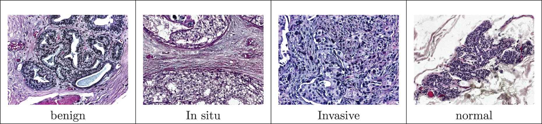
We aim to provide a complete classification that takes into account four cases of malignancy: normal, benign, in situ, and invasive cancer.
We develop a model based on parallel convolutional neural networks and combined deep features, to consolidate the machine learning training process. Previous works are based on stacked serial machines. In this novel architecture, we assembly the architecture of two conventional networks: Inception and Xception models. To the best of our knowledge, there is no existing researches presenting this architecture.
3.2. Dataset
We considered breast tissue biopsies stained with hematoxlin and eosin [22]. Breast tissue biopsies allows the pathologists to histologically assess the microscopic structure and elements of the tissue. During the biopsy, the tissue is stained with H&E and the nuclei are distinguished from the parenchyma. Therefore, the abnormalities can be assessed and categorized. Benign abnormalities represent non-malignant changes in normal structures of breast parenchyma. Malignant abnormalities are classified as in-situ carcimonia and invasive carcimonia. In the in-situ lesion, the cells are restrained inside the mammary ductal-lobular system. Cells are spread beyond the ducts in the case of invasive carcimonia. The BACH dataset was made available through the Grand Challenge on BC Histology images. It contains microscopy images annotated by expert pathologists. The dataset includes 400 images collected from different patients and presenting with four classes: Normal, Benign, In situ carcinoma and Invasive carcinoma. The images are 2048 by 1536 pixels, with spatial resolution 0.42 × 0.42 µm. The images were acquired using a Leica DM 20000 Led microscope and Leica ICC50 HD camera. Further description for the dataset is available in [23].
4. METHODOLOGY
In this section, we propose the new framework for the classification of histological images. The architecture is based on transfer learning using Xception and Inception Resnet. The two pre-trained convolutional neural networks, named backbone 1 and backbone 2 are used without the last fully connected layer. Their role is to perform feature extraction. The produced down sampled feature maps are dense presentations of the input images. The features are fed into a Global Average Pooling (GAP) layer. GAP processes a dimension reduction on feature maps and prepares the model for the final layers. The two outputs are concatenated and proceeded by the dropout layer and then the last dense layer. The first part acts as encoder and provide lower resolution image representation. The remaining part, is the decoder.
Conceptually, the approach is based on:
Initial preprocessing for image normalization and enhancement.
Image subdivision based on a regular grid.
Image augmentation.
Feature extraction based on transfer learning using two backbones.
Sub-image classification.
Image classification by majority vote and maximum probability.
The block diagram of the proposed approach is shown in Figure 1. Each step will be detailed in the following sections.
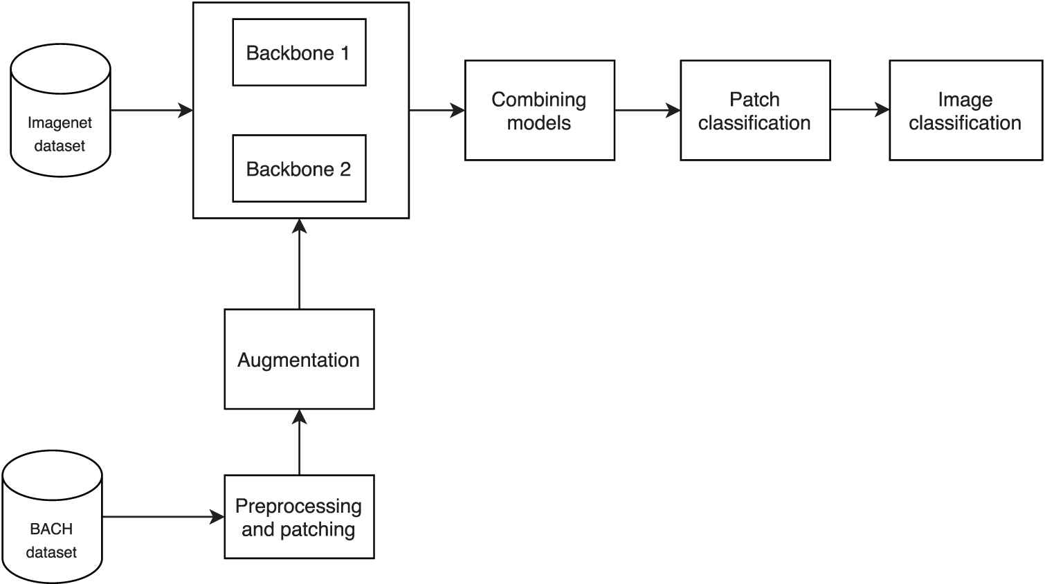
Block diagram of the classification pipeline.
4.1. Data Preprocessing, Patching and Augmentation
4.1.1. Preprocessing
Histological images show inter-images variability regarding contrast and color. Image normalization may improve the system robustness for the training stage as well as the prediction stage. Since staining, acquisition, and digitization process are performed in different conditions and laboratories, histopathological may show heterogeneity. The idea behind the normalization is to allow a robust classification framework and to avoid learning outfitting. We proposed a two-stage preprocessing based on Retinex illumination and the reflectance correction and then a histogram-based contrast enhancement technique.
The first preprocessing is based on the Retinex theory developed by Land and Mc-Cann in [24]. Retinex modelizes the visible disparity between the lightness perceived by the human eye and the absolute lightness incident on the eye. Experiments show that the human eye perceives relative lightness in local areas [25]. To achieve contrast enhancement, a logarithmic algorithm maps intensity using a response curve that simulates human eyes. The second preprocessing is an image normalization based on histogram technique. We apply a contrast histogram equalization to each color component [10]. Processing a global histogram equalization after contrast enhancement produces an over-enhancement with base extended smooth area and noise amplification in the image. These shortcomings are avoided and the artifacts in homogeneous area are minimized, thanks to the Level Adaptive Histogram Equalization (CLAHE). The algorithm is based on partitioning the image into equally sized tiles and the histogram equalization is performed locally. The histogram is clipped at a predefined value then a cumulative distribution function (CDF) is determined. The contrast enhancement for each tile is given by the slope of the CDF. Artifacts among neighboring tiles are minimized by interpolation or filtering [26].
4.1.2. Image subdivision
To reduce the complexity of the model and needed computing allocation, we subdivide our input images into 512 × 512 patches. The image is subdivided into patches images based on grid subdivision and nuclei density. The first method is based on subdividing the image into 12 patches. The nuclei based patching method is based on selecting patches with the entropy edges of the image. A sliding window process determines the non-overlapped patches with high entropy.
To reduce the complexity of the model and needed computing allocation, we subdivide our input images into 512 × 12 patches based on a grid subdivision into 12 patches.
There is no additional verification of the consistency of the sub-image regarding the diagnosis of the contained regions. For instance a sub-image obtained from a carcinoma image may contains regions with normal diagnosis.
4.1.3. Data augmentation
Data augmentation produces image samples for the learning process generated from the available dataset. In case of limited a dataset and missing generalization cases like different acquisition and digitization processes, the image augmentation is required to ovoid the classification overfitting. In the presented work, the data augmentation is based on geometric transform including rotation, flipping, and shifting. The intensity of original images are also shifted to simulate the acquisition process variability. Image shearing augmentation simulated also the physical properties of the breast tissue. These augmentations could not modify the malignancy category nor modify the image diagnosis result.
4.2. Transfer Learning
In handcrafted feature-based methods, the classifiers relay on the image singularities picked out provided by feature extraction algorithms to extract color region, tissue texture, local and global features, nulcei-based features, topological and morphological features, etc.
Unlikely, the DCNN allows to learn advanced and high-level features learned from the training dataset and there is no need to extract elaborate features before training the classifier. Furthermore DCNN-based approaches achieved high performance compared to handcrafted features-based approaches [27–30]. Using convolutional layers for feature extraction provides an efficient field-knowledge for the classification system. Followed by pooling layers, CNNs allow to reduce the field-knowledge needed to design a classification system. Thus, the performance of these methods is less biased by the used dataset and similar network architectures can achieve good results on different problems. The DCNNs, when applied in mammography and histology image processing, have improved the state-of-the-art results for CAD systems for BC diagnosis [11,14]. Te generated learning model performance depends widely on the learning dataset availability. Some classification problem have limited dataset and are unable to perform needed deep learning process. Moreover, data collection is expensive and may require specific and heavy acquisition process and expert annotation. Transfer learning aims to use a pre-trained model on large labelled dataset of a general context in order to overcome dataset availability problem. Only a minimal training adjustment is required to fit the new context.
Xception and Inception Resnet V2 are trained on the large Imagenet dataset [27] that contains over 15 million high-resolution images belonging to 22,000 categories. The two models have good accuracy on Imagenet dataset. The structure of the two CNNs is described as follows:
4.2.1. Inception ResNet architecture
The Inception architecture was first introduced by Szegedy et al. in 2014 [31], known also as GoogLeNet (Inception V1). The most recent version is Inception ResNet (Inception V4) delivered in 2016. An Inception model is a stack of building blocks called Inception modules. Inception modules are similar to convolutional feature extractors but cross-channel correlations and spatial correlations are decoupled. Inception Resnet V2 is based on the Inception architecture that have proven to achieve very good performance and low computational cost. Moreover, Inception Resnet V2 utilizes residual connections which avoids the degradation problem and reduces the training time compared to filter concatenation [31]. Compared to inception based architecture and hybrid inception versions, Inception Resnet V2 has improved recognition performance by the virtue of residual connections [31]. In Bianco et al. [32], authors present an in-depth comparison between several DNNs. The performances indices are regarding accuracy rate, complexity and computational resources usage (time, memory). Inception Resnet V2 performs the third best accuracy with lower computational complexity compared to NASNET- A-Large and SENet-154. The results are also similar regarding the accuracy density that measures how efficiently the model uses its parameters.
4.2.2. Xception architecture
Xception stands for Extreme Inception, The Xception model is based on linear stack of depthwise separable convolution layers where cross-channel correlations and spatial correlations are entirely decoupled [33]. This model is composed of 36 convolutional layers and each layer includes 14 modules. Each module, except for the first and last modules, has linear residual connections.
Xception model is among the best architecture regarding the accuracy, computational complexity and parameter usage efficiency. Xception architecture, based on depthwise separable convolution layers, outperforms VGGNet, Inception-v3, and ResNet [33]. While NASNET large and Senet-154 outperform all models, the number of parameters and model complexity is very huge.
4.3. Combining Models and Classification
The two pre-trained CNNs are used for deep feature extraction. Feature vectors are then reduced separately using the 2D GAPlayer. GAP layer is used to minimize the number of parameters and therefore to avoid the overfitting problem. The following figure explains the dimension reduction principle: each h × w feature map is replaced by single number computed as the average of [h w] values.
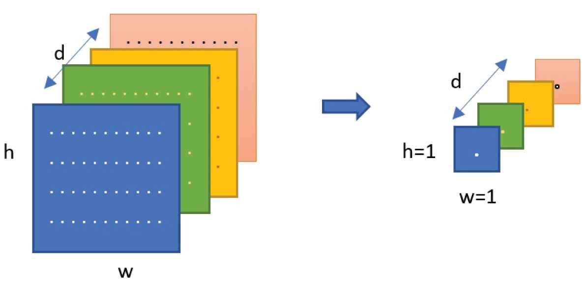
Global Average Pooling (GAP) Layer functionality.
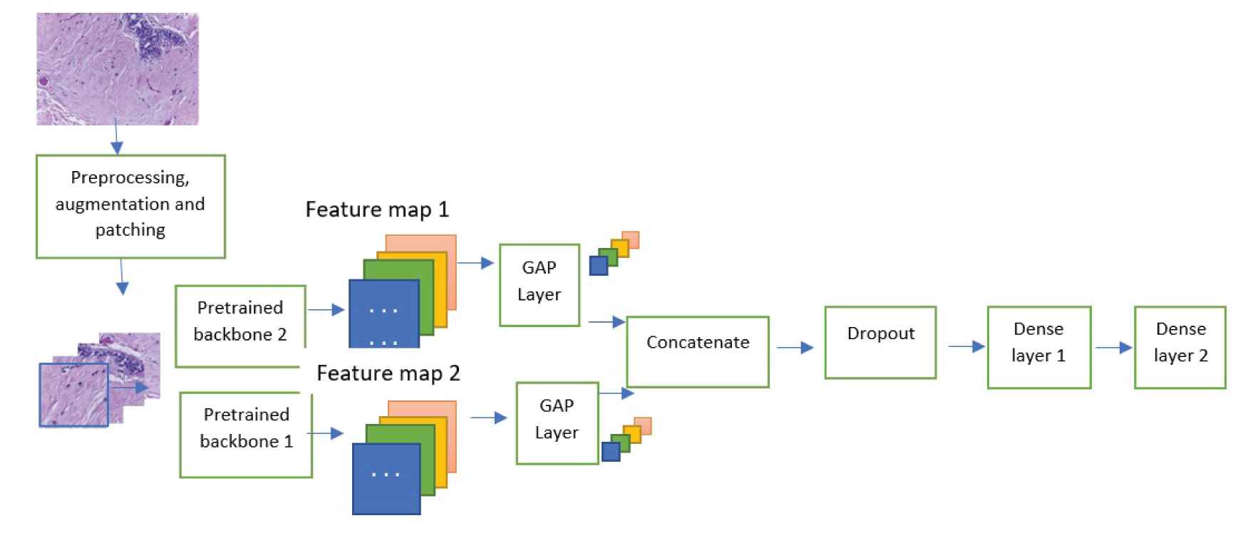
Overall architecture.
The resulting feature is an array containing d values where d is the number of filters. Introduced in [34], GAP replaces the traditional fully connected layer and provides more accurate classification. Moreover, the advantage of using GAP layer over a fully connected layer is the correspondence between feature maps and categories. GAP can be interpreted as a structural regularizer that explicitly enforces feature maps to be confidence maps of categories. The extracted features are concatenated to form 1024-dimensional feature vector. Since each CNN model captures feature information, concatenating two feature vectors generated by different models provide more discriminative representation.
4.3.1. Dropout and bagging
Learning overfitting and training time are common problems in machine learning and especially in DCCNs. Furthermore, combing the outputs of separated trained models is computationally expensive [35]. To address these issues,we perform a dropout method before feeding the concatenated feature vector into the last fully connected layer.
Dropout is a technique that addresses the overfitting problem as an effective regularization and provides a away of combining different neural networks models efficiently [36,37]. Dropout is widely adopted in the training of deep neural networks as an effective regularization and implicit model ensemble method. Dropout also improves the generalization ability as demonstrated in [38]. During this process, each node is dropped out randomly with a given rate. The rate can be chosen using a validation set. It can also be set to a fixed rate, usually 0.5 for retaining the output of the node. This process is done only during the training time [37]. Nodes not set to 0 are scaled by (1/(1-rate)) to maintain the same sum over all inputs.
An alternative solution to the dropping is Bagging, known also as bootstrap aggregating. Bagging is an ensemble learning method based on training the models on sampling subsets from the training sets [39] where missing entries are duplicated from the selected subset. This sampling way will allow different predictors models that will be used for an aggregate predictor. However, the bagging requires high computational capabilities as each model needs to be updated simultaneously.
4.3.2. Densely connected layers
The concatenated features are fed to two dense connected layers followed by a SoftMax logistic regression layer. The reason behind using two fully connected layers is to enrich the learning ability and to adopt the generic features to our histopathology dataset. Figure 3 illustrates the overall architecture of the proposed network.
In order to combine classification result of the patches, the original image classification is obtained by two ways:
Maximum classification probabilities of patches.
Majority vote of patches labels.
5. RESULTS
In this section, we present the results obtained for the BACH dataset. The assessment is performed for sub-image classification and for whole image classification.
5.1. Experimentation Settings
The histological dataset, available at [40], is composed by 400 high-resolution H&E stained histology microscopy images. The four classes are equally presented (100 images for each category) and annotated by two experts pathologists and without any cases of disagreements. Images are.tiff format and have a size of 2048 × 1536 pixels. A pixel represents 0.42 µm × 0.42 µm. Figure 4 highlights the variability of stain shades.
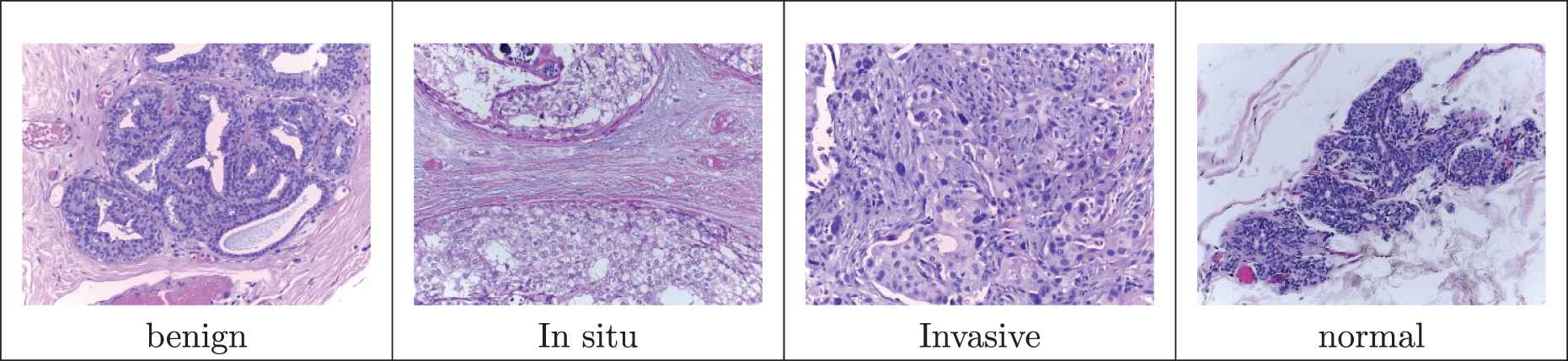
Samples of hematoxylin and eosin (H&E) microscopic biopsy images from the used dataset (Original images).
The model is used first for classifying 512 × 512 histology sub-images into four tissue classes (normal, bening, in situ carcinoma, and invasive carcinoma). The proposed model is trained on 80% of the training set while 25% of the training set are used for validation step. The statistics about the training, test and validation for the sub-images datasets are detailed in Table 1.
Prior to learning and classification steps, the input images are processed with the presented preprocessing method. Figure 4 represents the input image and Figure 5 the preprocessed enhancement results. Retinex algorithm allows to stretch and correct the illumination and to correct the reflectance which improves the visual effects. Based on guided filtering, as presented in [41], Retinex allows edge-preserving ability and solves the problem of over-enhancement due to unreasonable estimation model of luminance. After that, the obtained image is processed by CLAHE which enhances the contrast locally by redistributing the pixel values in image tiles and bringing out further image singularities. The combination of the two enhancement approaches allow to achieve an improvement in image contrast of about 58%.
Image data augmentation used to expand the dataset is obtained using the deep module ImageDataGenerator. This Keras module generates real-time image samples using the specified parameters. Batches of tensor image data are generated with real-time data augmentation which allows new variations of the training dataset during the training epochs. We specified the following parameters for the augmentation module: horizontal flip, vertical flip, rotation range equal to 180 which corresponds to a random rotation angle between −180 and 180 degrees, width and height shift range of 0.3 which corresponds to the fraction of random shift of the image. We performs also a a channel shift range of 0.3 that randomly shifts the channel values and a finite shear transform that stretches the image at a small angle. We initiate the two DCNNs using the pre-trained models on ImageNet dataset. We concatenate the obtained feature maps from the two deep backbones and perform the 2D GAP transform. A dropout of 0.5 prevent the overfitting of the training process. Networks weights are updated using an adaptive learning rate gradient-descent back-propagation algorithm [42]. We selected the categorical cross-entropy loss function and the adaptive moment estimation algorithm (Adam) in order to perform the optimization during the training process. We tried different learning rates (0.001, 0.0001, and 0.00001), the tested batch sizes are 8, 16, and 32. The tuning process leads to the optimal batch size of 32 and the learning rate of 0.0001 with a decay of 0.00001. the number of iterations per epoch is 100. The loss function computes the cross-entropy loss between the labels and predictions for the training set and the validation set. The training process takes end after the stabilization of the four classes which is 60 epochs. The accuracy curves of the fine-tuned model are illustrated in Figure 6, correspondent loss curves are presented in Figure 7.
| Number of Images | Percentage | |
|---|---|---|
| Training | 2880 | 60 |
| Validation | 960 | 20 |
| Test | 960 | 20 |
| Total | 4800 | 100 |
Datasets statistics for training, validation, and testing.
Preprocessed images.
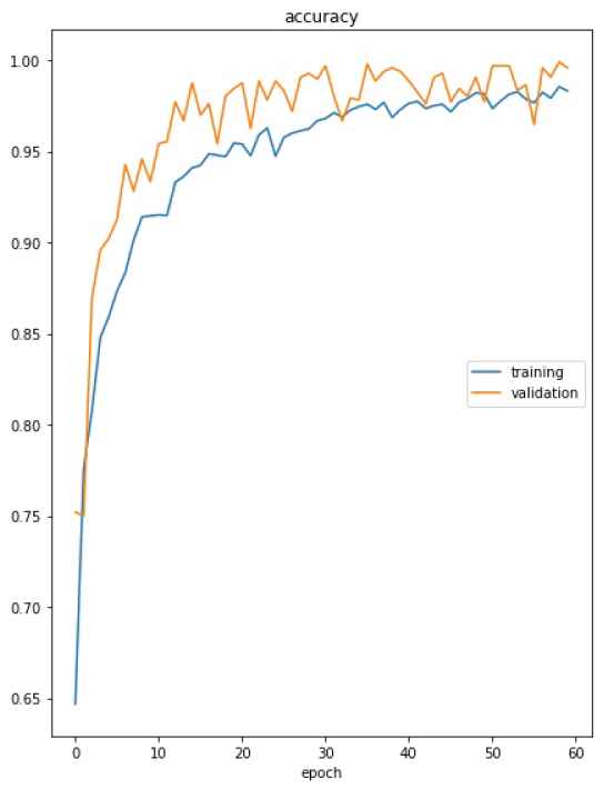
Training and validation curves of accuracy for the fine-tuned and trained deep architecture.
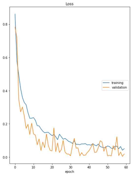
Training and validation curves of loss for the fine-tuned and rained deep architecture.
5.2. Sub-images Classification
First, the image classification is performed with sub-images classifier. Then, the image-wise classification is obtained by combining the patch classification results. The classification efficiency relies on the extraction of nuclei features and tissue organization. Carcinoma and non- Carcinoma categories can be separated based on the features of the nuclei. Color, shape of the nuclei, density, and variability are also determinant for the classification decision. Invasive and In situ classes are well identified when analyzing the tissue structure. learning transfer, dataset augmentation will allow to ovoid the overfitting problem by increasing the dataset and enrich the learning process.
The sub-images are obtained by subdividing the original whole image (2048 × 1536) into 12 contiguous and non-overlapping sub-images of 512 × 512. This subdivision will not impact the feature extraction process as the nuclei radius ranges for 3 to 11 pixels. The sub-images classification prediction for the test dataset is obtained using the presented deep model. The overall accuracy is 97.29%. Specifically, for the carcinoma cases, the achieved sensitivity is 99.58%. The confusion matrix for the four malignancy levels is presented in Table 2. The rows in the confusion matrix refer to the ground truth image label while the column indicate the classifier result. The True Positive Rate (TPR) for a specific class represents respectively the rate of samples correctly identified as belonging to this class in relation to the current number of samples belonging to this class. TPR is known also as the classifier sensitivity. The False Negative Rate (FNR) for a specific class in the rate of the samples not identified as belonging to this class in relation to the current number of samples belonging to this class. TPR and False Positive Rate (FPR) are depicted in Table 3. The sensitivity is above 99% for carcinoma classes while normal and benign classes achieve a sensitivity of 95%.
| Benign | 228 (95%) | 11 (4.58%) | 0 (0%) | 1 (0.41%) |
| In situ | 1 (0.41%) | 238 (99.16%) | 1 (0.41%) | 0 (0%) |
| Invasive | 0 (0%) | 0 (0%) | 240 (100%) | 0 (0%) |
| Normal | 10 (4.16%) | 1 (0.41%) | 1 (0.41%) | 228 (95%) |
Confusion matrix for sub-image classification.
| Class | TPR | FPR |
|---|---|---|
| Benign | 95% | 5% |
| In situ | 99.16% | 0.83% |
| Invasive | 100 % | 0% |
| Normal | 95% | 5% |
TRP, True Positive Rate.
Obtained TPR and FPR for sub-image classification.
5.3. Whole Image Classification
During the whole image subdivision, there is no guarantee that the patch will include determinant diagnosis information. Therefore, the fusion process will provide image classification reliability for the original whole image.
Classification by maximum probability: the maximum probability of classified patches decides the image label.
Classification by majority vote: the label that has the most accuracy within the twelves sub-images decided the image label.
To reinforce the sensitivity of our approach for carcinoma detection, the fusion decision unresolved cases (specifically for majority vote) are resolved in this order: invasive, in situ, benign, and normal. This mean that in case of having 6 sub-images classified as invasive and 6 subclasses classified as in situ, the final decisions will considerate the label invasive as final decision. Similarly, in case of probability equality in the maximum probability based fusion method, the fusion method selected the decision with the provided priority. In fact, sensitivity is of great interest when addressing medical classification problem, therefore we prioritize malignant classes. As the proposed CAD is an additional opinion or a pre-diagnosis system, favoring the carcinoma classification in detriments of normal and benign decision will reduce the carcinoma false negative.
The whole image classification are detailed in Table 4. The two fusion approaches lead to an overall accuracy of 100% and 95% for respectively the majority vote and the maximum probability decision. In a two problem classification, the cancer cases and non-cancer cases accuracies achieved respectively 100% and 97.5% by majority vote. Maximum probability performs worse than majority vote and is not suitable for illness classification problem. The overall accuracy is better in the whole image classification compared to the overall accuracy for sub-image classification when we use the majority vote strategy. This is explained by the fact that the image abnormalities are randomly presented in the image and the image subdivision is not guided by the presence of abnormalities. Moreover, normal tissue coexists within abnormal cases. The sensitivity of our method for cancer cases achieves 100%, and achieves 95.6% for non-cancer cases by majority vote which is encouraging for using this approach as a secondary decision system.
| Class | Accuracy Obtained by Majority Vote (%) | Accuracy Obtained by Maximum Probability (%) |
|---|---|---|
| Benign | 100 | 95 |
| In situ | 100 | 95 |
| Invasive | 100 | 90 |
| Normal | 100 | 100 |
Whole image classification results.
5.4. Comparison with Similar Works
In Araújo et al. [22], the authors proposed a CNN and a CNN+SVM based approach to classify the same dataset. The feature extraction is performed by the CNN and the extracted features are used for the two classifiers. The image classification accuracy achieved 77.8% for four classes, while the achieved sensitivity was 95.6% for cancer cases. The classification of two classes invasive and noninvasive tissues achieved 83.3%. In the work of Fondon et al. [10], an enhanced feature extraction approach is presented. Three sets of features were selected respectively related to the nuclei properties, the color and the texture. The built feature vector is fed to a quadratic SVM. The overall accuracy reaches 76% and the sensitivity for cancer cases is 92%. In Yao et al. [43], the authors proposed a parallel structure that consists of a DCNN and a recurrent neural network for image feature extraction, then a specific perceptron attention mechanism is used to unify the derived features. The overall accuracy reaches 97.5%.
The ensemble of fine-tuned VGG-16 and VGG-19 models offered sensitivity of 97.73it offered an F1 score of 95.29.
The results comparison demonstrate that our model significantly outperforms state-of-the-art feature-based methods. Moreover, it performs better than recent deep learning-based methods. In addition, our approach provided four classes classification and is not limited to cancer and non-cancer cases. In our dataset, the patch-wise were obtained by a grid-subdivision and there is no available specific ground truth for these patches other than the WSI ground truth. This may lower the patchwize classification accuracy as some patches may not contain relevant information for the training as well as for the testing dataset.
6. CONCLUSION AND FUTURE WORK
We proposed a deep architecture for the classification of BC based on H&E stained histological imagery. The approach provides the breast imagery classification into normal tissue, benign, in situ carcinoma, and invasive carcinoma. The virtue of our architecture is to provide a new deep architecture based on two deep networks Xception and Inception Resnet V2. The backbones are pre-trained on a large dataset to overcome the limited size of available histological dataset. The extracted features are then reduced using the two-dimensional GAP layer. A dropout layer allows to reduce the model complexity and then the features are fed to two densely connected layers. The virtue of our approaches is to take advantages for two semantic deep features as well as the transfer leaning method. The obtained model allows to discriminate the nuclei features and tissue properties. Compared to existent researches, the performance of our approach outperforms state-of-the-art methods. Our approach can be extended for WSIs where image may contain multiple pathology regions.
CONFLICTS OF INTEREST
The authors declare no conflict of interest.
AUTHORS' CONTRIBUTIONS
Methodology and software: Hela Elmannai; formal analysis and validation: Monia Hamdi and Abeer AlGarni; writing: Monia Hamdi and Hela Elmannai; project administration: Abeer AlGarni; funding acquisition, Monia Hamdi.
ACKNOWLEDGMENTS
The authors would like to thank the Center for Promising Research in Social Research and Women's Studies Deanship of Scientific Research at Princess Nourah University for funding this Project in 2020.
REFERENCES
Cite this article
TY  - JOUR
AU  - Hela Elmannai
AU  - Monia Hamdi
AU  - Abeer AlGarni
PY  - 2021
DA  - 2021/03/08
TI  - Deep Learning Models Combining for Breast Cancer Histopathology Image Classification
JO  - International Journal of Computational Intelligence Systems
SP  - 1003
EP  - 1013
VL  - 14
IS  - 1
SN  - 1875-6883
UR  - https://doi.org/10.2991/ijcis.d.210301.002
DO  - 10.2991/ijcis.d.210301.002
ID  - Elmannai2021
ER  -