
A Repairing Artificial Neural Network Model-Based Stock Price Prediction
- DOI
- 10.2991/ijcis.d.210409.002How to use a DOI?
- Keywords
- Stock price; RANN; Learning algorithms; Self-organizing; Dynamic
- Abstract
Predicting the stock price movements based on quantitative market data modeling is an open problem ever. In stock price prediction, simultaneous achievement of higher accuracy and the fastest prediction becomes a challenging problem due to the hidden information found in raw data. Various prediction models based on machine learning algorithms have been proposed in the literature. In general, these models start with the training phase followed by the testing phase. In the training phase, the past stock market data are used to learn the patterns toward building a model that would then use to predict future stock prices. The performance of such learning algorithms heavily depends on the quality of the data as well as optimal learning parameters. Among the conventional prediction methods, the use of neural network has greatest research interest because of their advantages of self-organizing, distributed processing, and self-learning behaviors. In this work, dynamic nature of the data is mainly focused. In conventional models the retraining has to be carried out for two cases: the data used for training has higher noise and outliers or model trained without preprocessing; the learned data has to update dynamically for recent changes. In this sense, propose a self-repairing dynamic model called repairing artificial neural network (RANN) that correct such errors effectively. The repairing includes adjusting the prediction model from noise, outliers, removing a data sample, and adjusting an attribute value. Hence, the total reconstruction of the prediction model could be avoided while saving training time. The proposed model is validated with five different real-time stock market data and the results are quantified to analyze its performance.
- Copyright
- © 2021 The Authors. Published by Atlantis Press B.V.
- Open Access
- This is an open access article distributed under the CC BY-NC 4.0 license (http://creativecommons.org/licenses/by-nc/4.0/).
1. INTRODUCTION
Financial data gains more attention by the research and business people across the world, it is highly volatile time series data, analyzing it would help to improve the commerce in many ways. The market process that handles the long term financial instrument is known as capital market. These instruments could be stocks, mutual funds, bonds, equities, trades, and derivatives. These funds are the investments received from the public and used as the company's capital resource. People make their investment decisions based on returns and risk of each instrument. One major instrument is stock, buying and selling are the two major activities performed over these funds. Every day, the stock price varies depends on its demand and supply that are influenced by various factors like currency rate, inflation, and social and political conditions. The stock market index represents the trend of stock price oscillation. Predicting the direction of such a trend is attracted by many researchers. The public or the investor can be benefited from an accurate forecast of the stock index trends. The stock market forecasting could be divided into two types of analysis: fundamental analysis and technical analysis. Fundamental analysis dealt with the basic financial data of organizations like money supply, earnings, interest rate, inflation rate, cash flow, price-earnings ratio, the book to market ratio, and returns. Technical analysis is to handle rational data like the correlation between the indicators, price, and volume.
Stock price forecasting is achieved by identifying the patterns and trends of the time series data. Hair et al. [1], reported that multiple regression methods are suitable for financial data analysis, especially for stock price forecasting. However, the performance could be degraded when the data become more complex [2]. Mendenhall et al. [3], testified that the regression models are helpful to prone linear patterns only, whereas the stock market data is nonlinear in general. Hence, the neural network (NN)-based approaches are more appropriate for forecasting the series. The main advantage of NN is that they are able to build a nonlinear model without requiring a priori knowledge about the transactions. Moreover, the NN follows a nonparametric approach, as it reduces the complexity of the training. Other models such as support vector machines (SVMs) with handcrafted features [4,5], random forests [6,7], ensemble of the same classifiers [8], integration of different classifiers [9], and the most advanced and recent one is the deep learning networks [10,11] are the evidence of the progress in stock price forecasting problem. In continuation, the other recent works Chong et al. [12], Gudelek et al. [13], Hiransha et al. [14], and Barra et al. [15], depict the research focuses on exploring various network framework and methods in stock market domain.
Most of the prediction models continued after ensuring that the data is clean and noise-free. However, when some of the data samples could be found incorrect or corrupted while building the model, at that time the erroneous sample would have been used for training the prediction model. Now, it is necessary to remove or correct the model as the incorrect data might have infected the model. One solution is to rebuild the model from scratch to resolve this issue, however, it involves greater time complexity. This work, propose a new solution called a repairing artificial neural network (RANN) for handling such dynamic situation with the trained model without rebuilding it from the scratch. The complete repairing model is to adopt the dynamic nature of the data. Though the data could be pre-processed in the early step, there might be need for adding or removing attributes over a period of time. For adding such trendy data or removing the outdated data from the trained model, RANN would be more useful as demonstrated.
The rest of the paper is organized as follows: The following section presents a summary of related works on neural-network-based stock price forecasting methods. Section 3 introduces the concept of an artificial NN. Section 4 explains the proposed RANN to handle dynamic data changes while learning. Section 5 discusses the experimental setup. Section 6 presents the quantified results and discussions. Section 7 concludes the paper.
2. RELATED WORKS
Stock selection has become a gradually hot subject in the field of finance research, as current interesting studies and works reviewed below:
Vaisla and Bhatt [16] have compared the stock price prediction performance from the NN and statistical technique. The performance is analyzed with various parameters like mean square error (MSE), mean absolute error (MAE) and root mean square error (RMSE), the results indicate that the NN-based stock market forecasting has better accuracy than the statistical methods like regression analysis. Dase and Pawar [17] have conducted a study on the application of ANN for stock market forecasting. This study concludes that the ANN-based stock price prediction models have the ability to achieve better accuracy than other techniques. Liao and Wang [18] proposed a NN model with stochastic time effective function. The investigation results indicated that this model is more effective than conventional NN models. Mostafa [19] has applied both multi-layer perceptron (MLP) NN and GRNN for forecasting the Kuwait stock exchange (KSE) data. The simulation results shown that GRNN outperforms the conventional regression and ARIMA models in stock price prediction. Lu [20] have presented an NN-based stock price forecasting model integrated with a denoising method. Independent component analysis (ICA) is used here for denoising. The investigation's results indicate that the denoised data improves the NN prediction, and reported that ICA-based denoising outperforms the wavelet denoising technique.
The major objective of stock price forecasting is to reach better prediction accuracy with minimum training data as well as with a simple learning model. The authors [21,22] have proposed an prediction models called and autoregressive integratedmoving average (ARIMA) and cerebellar model articulation controller neural network (CAMC NN) for stock index prediction. The experimental results estimated with the Taiwan stock exchange (TSE) index indicate that CAMC-NN achieves better prediction than SVR and BPNN models.
Hadavandi et al. [23], have presented a hybrid forecasting model, where ANN is integrated with genetic fuzzy systems (GFS). The investigation results indicate this model outperforms the other existing models in terms of MAPE.
Different hybrid prediction models were used in different studies by integrating with optimization and intelligence algorithms. The authors [24–26] have proposed a models by using artificial fish swarm algorithm (AFSA), genetic algorithm (GA), and generalized auto regressive conditional heteroscedasticity (GARCH). The results have shown that the proposed models outperforms than existing ones. Chopra et al. [27], presented a hybrid MLP-NN with LM algorithm for stock market prediction, and the results indicate the significance of adding more neurons in the hidden layer. Chandar et al. [28], have implemented a hybrid NN model with a wavelet transform technique for stock index prediction. Here, the wavelet transform is used to decompose the time series data, further, the received wavelet components are used as input variables for building the forecasting model based on NN. Investigation results indicate the significance of wavelet components toward improving greater forecasting accuracy.
Fang et al. [29], have proposed a hybrid wavelet neural network (WNN) model with hierarchical GA (HGA) for stock index prediction. Here, the WNN architecture is evaluated with minimal hidden neurons and reported a better prediction accuracy. Chen et al. [30], applied recurrent neural network (RNN) for stock price forecasting and reported better performance with Chinese stock market data. Pang et al. [31], have presented an long short-term memory (LSTM) model for stock index prediction and evaluated through financial analysis. The experimental results are received from real-time data and reported that the LSTM model outperforms the artificial neural network (ANN) model. Chi [32] have presented a BPN for stock price forecasting and reported with better prediction accuracy, and it is suggested to add more attributes which are having a strong influence on the stock market. Lei [33] have proposed a hybrid model with rough set (RS) and WNN for stock price prediction. Here, RS is used for dimensionality reduction, followed by WNN is implemented as a prediction model. The performance of RS-WNN is studied and compared with other classifiers such as SVM and conventional WNN, the results indicate the effectiveness of the proposed method.
Yang et al. [34], have presented an extreme learning machine (ELM) model for stock price forecasting as well as for stock scoring. The experimental results indicate the effectiveness of the learning model and state the robustness of ELM with greater prediction accuracy. Li et al. [35], proposed a deep reinforcement learning (DRL) architecture for stock price prediction problem and demonstrated the feasibility of the DRL method against the Adaboost algorithms. Qiu et al. [36], compared the stock price prediction performance of LSTM, LSTM with wavelet transform, and gated recurrent unit (GRU) NN model. The simulation results indicate that the LSTM model achieves better prediction accuracy of 94% while reducing the error rate to 0.05. Kim and Kim [37] proposed an integrated LSTM-CNN model for stock price prediction. The experimental results indicate that this integrated model outperforms the individual model. Dai and Zhu [38] fused the sum-of-the-parts (SOP) method with ensemble empirical mode decomposition (EEMD) to forecast stock market returns. The simulation results indicate the promising results on return predictions. Carta et al. [39], proposed an ensemble of deep Q-learning for stock price forecasting. This method avoids over-fitting, and do not use market annotations, and used ensemble of reinforcement learning for better prediction. The performance study indicate the significance of Q-learning with higher prediction accuracy.
Ibidapo et al. [40], presented a comprehensive review on applying soft computing techniques for stock market prediction and reported that the hybridization of ANN with soft computing algorithms outperforms better than the conventional machine learning algorithms. Yoon et al. [41] investigated NN and GA in short-term stock forecasting domain. The experimental results show that the GA-based on backpropagation NN model has a significant improvement in stock price index series forecasting accuracy. Cai et al. [42] presented a new fuzzy time series model combined with ant colony optimization (ACO) and auto-regression. The ACO is adopted to obtain a suitable partition of the universe of discourse to promote the forecasting performance. Siddiqueet al. [43], proposed a hybrid stock value forecasting model with support vector regression (SVR) integrated with particle swarm optimization (PSO). Empirical results show that the proposed model enhances the performance of the previous prediction model.
3. ARTIFICIAL NEURAL NETWORK
NN models have been widely applied for stock market forecasting as they are robust with noisy data, moreover, the generalized regression neural network (GRNN) has been successfully implemented for a wide range of stock market predictions applications. Devadoss and Ligori [44] listed the features of ANN as follows:
ANN doesn't require any prior knowledge about the data as it learns from samples.
ANN models can produce better generalization even with noisy data.
ANNs are nonlinear, hence it is more suitable for Stock price forecasting.
Figure 1 depicts a function of a single artificial neuron, which is also known as a perceptron in the ANN domain.
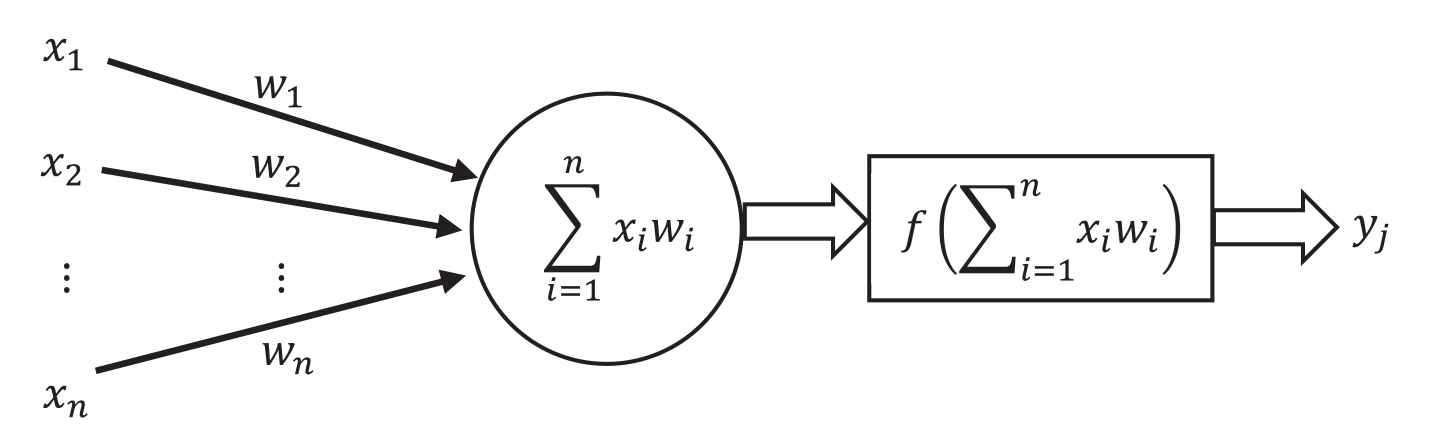
Systematic diagram for neural network.
The connection between each neuron is assigned with a real number known as weights
Artificial neuron or perceptron is the basic computation element of an ANN. The objective is to learn the optimal weights between perceptron, this process is known as a training or learning step. There are two types of architecture: single-layer perceptron (SLP) and MLP. SLP consists of two layers: the input and output layer, the input layers receive the input data samples and the output layer estimates the result of the NN.
The SLP architecture is able to build a decent generalization model, however, they are suitable for linearly separable problems. MLP is used to learn nonlinear data samples. A backpropagation learning-based neural network (BPN) is utilized as a classifier. The BPN follows the three-layer architecture of MLP, consists of an input, a hidden, and an output layer. For the stock price forecasting problem, the number of neurons in the input layer and the hidden layer is kept equal to the number of input variables
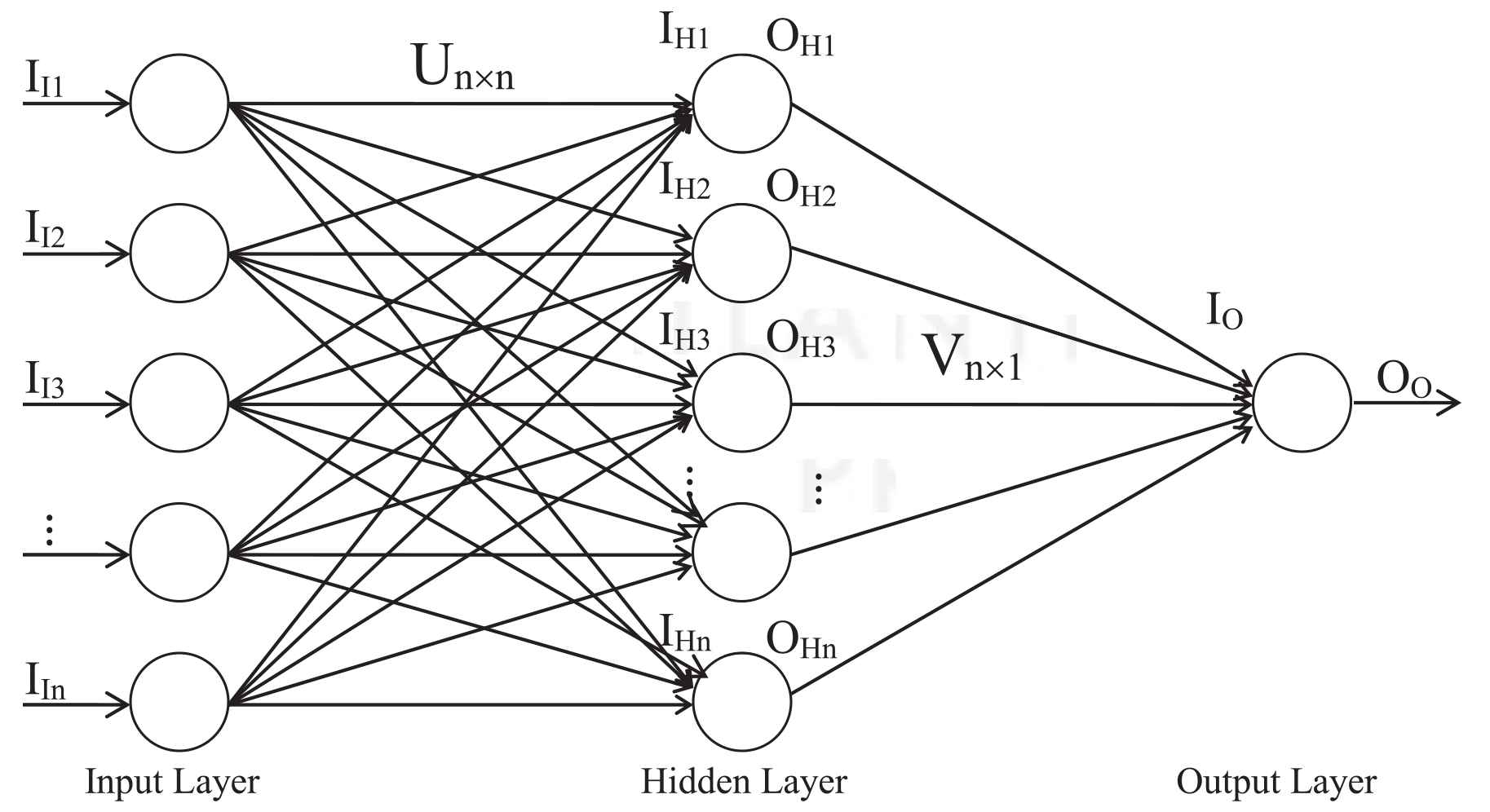
Backpropagation neural network.
Once the architecture is established, then the two-weight matrices: weights between the input layer and hidden layer
After the initialization step, a set of data samples is partitioned from the dataset that is to be used for training. With the set of training samples, a single learning step is described in the following text.
From this training dataset, a data sample of input variables is fed to input layer
In the next step, the input to the hidden layer
Then the output of the hidden layer is estimated with a “sigmoid” activation function as given below
Further, the input to the output layer,
And the output of the output layer is estimated by applying sigmoid function over its input, defined as
The output of the NN
The weight updation based on the backpropagation learning approach is given below. At first, the weights between the hidden layer and output layer
With the weight update estimates, the weight matrices are updated.
ANN models have many advantages as highlighted in the related works section, however, these models can't handle dynamic changes of the dataset. For example, while learning the
4. PROPOSED RANN MODEL
In conventional models the retraining has to be carried out for two cases: the data used for training has higher noise and outliers or model trained without preprocessing, the learned data has to update dynamically for recent changes. In this sense, propose a self-repairing dynamic model called RANN that correct such errors effectively. The following are the chances of dynamic changes which would infect the learning model, as the samples have been learned already
Case 1 – There might be a change in an attribute value
Case 2 – There might be a change in more attribute values
Case 3 – There might be a change in the decision values
Case 4 – There might be a need for eliminating row(s) of the sample, as it might be outdated
Case 5 – There might be a need for removing an attribute (column)
Case 6 – There might be a need for adding an attribute (column)
These problems are addressed in the proposed RANN model.
The proposed RANN learning model focuses on renovating the ANN learning model while adopting the dynamic behavior of the data samples. For the proposed RANN model, the initial weight matrices
Case 1 – There might be a change in an attribute value, as it has been learned already
Once the training is over or in progress, when it is found that an attribute value
With these two sets of weight matrices, the difference of weights are estimated, and added to the current weigh matrices
The weight difference between the weight matrices
After the adjustment of current weight matrices, the training phase continued either with the last training sample if the training is over, or with the next training sample if the training is in progress.
Case 2 – There might be a change in more attribute values
The previous case deals with the change in the single value of a single attribute. The dynamic changes could happen with more values of the same attribute or multiple attributes. To adopt such changes to the learning model, the current learning model
Case 3 – There might be a change in the decision values or output classes.
For the real-time data, the dynamic changes could happen with the class labels of decision values. For the past two cases, the changes in the input variables are handled, this case deals with the output variable of the network. The basic weight updation procedure similar to the previous two cases is followed, except that all the elements of
Case 4 – There might be a need for eliminating row(s) of the sample, as it might be outdated.
For a nonlinear time-series data, the learning model has to adopt the new samples every time, and the same time the past or outdated data has to be removed from the trained model to align the model perfectly with the current trend. Hence, it is necessary to remove the outdated sample from the learned model. Once again, the similar weight updation process is followed with minimal changes from the previous equations. The outdated samples are received from the original dataset and stored as a separate dataset
Case 5 – There might be a need for removing an attribute (column)
Recently the dimensionality of the data is growing exponentially that increases the memory and computation requirements. One common solution is to apply feature selection methods to identify and keep the most relevant features and discard the remaining. In general, feature selection methods are to be executed before the classification process starts. Suppose a relevant feature could be identified as outdated later on, in such a situation the architecture of the classifier has to be renovated to remove such features from the current learning model. This case addresses the issue of removing an input variable from the learned NN model. At first, the current learning model is suspended and the current weight matrices
For an illustrative example, consider the given weight matrix of size
To remove the 3rd attribute, the corresponding row & column is removed the weight matrix to scale it down to
Further, each element of the reduced matrix is added with the average fraction of the elements from the removed row and column, defined as
The
With the scaled-down weight matrices
Case 6 – There might be a need for adding an attribute (column)
Scalability is an important issue of real-time datasets since the dimensionality could be increased in horizontal and vertical directions. In the case of a vertical increase, the number of samples gets added to the dataset, and for horizontal growth, the number of attributes is added to the dataset. The NN model can adopt the new samples incrementally as they are received, this way the vertical growth of the data can be handled effortlessly. However, for the horizontal growth of the data, when a new attribute is about to be added to the existing dataset, the NN architecture should be repaired to accept the new input variable. Adding an artificial neuron to the input and hidden layer would make the NN model accept the new attribute. However, assigning the weights for the new connections from the recently added neuron to the other neurons in the hidden layer, and similarly assigning the weights from the existing input neurons to the latest neuron in the hidden layer is the problem to be addressed here. For this case, the current weight matrices are scaled up from
For an illustrative example, consider a
Adding a new element at the last would introduce the 5th row and column, the weights assigned for them are the mean of elements in the corresponding row and column. The
Similarly the other weight matrix
After scaling up the weight matrices, the learning process is continued with the current sample consists of the new variable. The backpropagation procedure estimates the optimal weights as discussed before.
The following algorithm summarizes the proposed RANN model-based learning for all the six cases to handle the dynamic data.
Algorithm– Repairing Artificial Neural Network Model
Inputs – Initial weights
Outputs – Repaired weight matrices
For any of the dynamic data updates, suspend the current learning model, and store its weights.
Follow the corresponding cases to handle the dynamic update.
Case 1 – To correct an erroneous attribute value
Construct and initialize a new learning model,
Learn the weights for the correct sample,
Re-initialize the learning model,
Learn the weights for the erroneous sample,
Update the corresponding element's weight at the current weight matrices
Case 2 – To correct a set of an erroneous attribute value
Collect the data samples with the incorrect attribute values,
Learn the optimal weights with a new learning model,
Collect the data samples with the correct attribute values,
Learn the optimal weights with a new learning model,
Update the corresponding element's weight at the current weight matrices
Case 3 – To correct a set of erroneous samples with incorrect decision values
Collect the data samples with the incorrect decision attribute values,
Learn the optimal weights with a new learning model,
Collect the data samples with the decision correct attribute values,
Learn the optimal weights with a new learning model,
Update all the elements of the current weight matrices
Case 4 – To eliminate a set of data samples
Collect the outdated data samples,
Learn the optimal weights with a new learning model,
Update all the elements of the current weight matrices
Case 5 – To remove an attribute from the dataset
Remove the corresponding row and column of weight matrices representing the input variable
Update the other elements by distributing the average fraction of eliminated elements from the corresponding rows and column as given in the Equations (27) and (30)
Case 6 – To add an attribute from the dataset
Add a new row and column to the current weight matrices.
Assign the new elements by taking the mean of existing elements in the corresponding rows and column as given in the Equations (33) and (35)
After updating the current weight matrices, the learning procedure is continued with the current learning model
5. EXPERIMENTAL SETUP
5.1. Datasets
The performance of the proposed RANN model is evaluated with five different stock market index datasets: Nifty50 (N50), Nifty-Bank (NB), Nifty-Pharma (NP) from www.nseindia.com, and BSE-IT (BIT) & BSE-Oil-Gas (BOG) from www.bseindia.com. For each dataset, a collection of the last five years' historical index data from January 1, 2015 to December 31, 2019 is collected. The offered datasets contain attributes like index data, open, high, low, and close indices. The stock index variables such as open, high, low, and close are considered as input variables to the NN. Along with the index variables, few more technical indicators are estimated and considered as input variables for the prediction model. The closing stock index trend for all the five market data are shown in the following Figure 3.
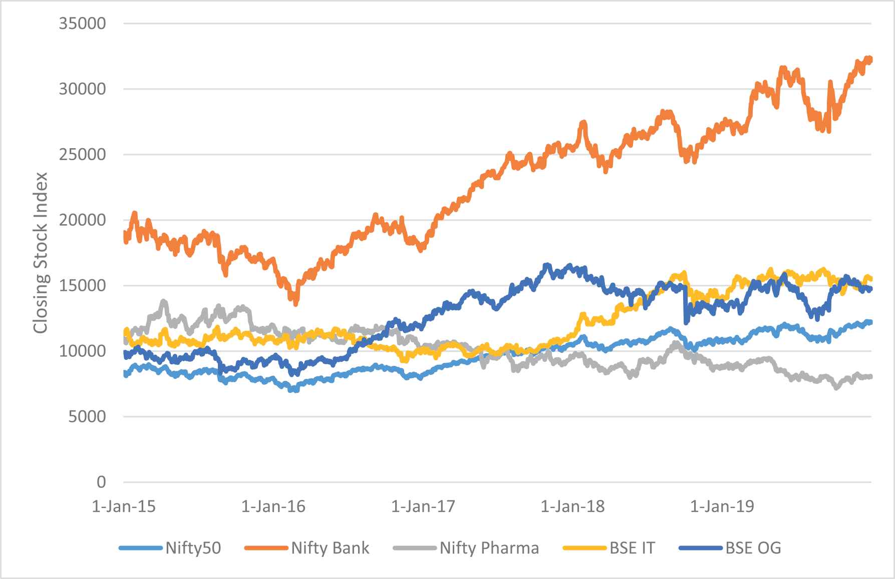
Closing stock price trend.
5.2. Technical Indicators
Three sets of technical indicators (input variables) are used to evaluate the performance of the proposed RANN model. Group 1 variables consist of 4 index variables and 12 indicators as listed in Table 1 as given in Shen et al. [24], Group 2 variables consists of 4 index variables and 24 indicators as listed in Table 2 as presented in Chang [45], and Group 3 variables consist of 4 index variables and 12 indicators as presented in Table 3 as listed in Mingyue et al. [46].
| Input Variables | Technical Indicators | Formulas |
|---|---|---|
| OBV | On balance volume | |
| MA5 | Moving average for 5 days | |
| BIAS6 | Bias | |
| PSY12 | The psychological line for 12 days | |
| ASY5 | Average stock yield of 5 days before the forecasting date | |
| ASY4 | ASY of 4 days before the forecasting date | |
| ASY3 | ASY of 3 days before the forecasting date | |
| ASY2 | ASY of 2 days before the forecasting date | |
| ASY1 | ASY of 1 day before the forecasting date | |
| CI3 | Closing indices of 3 days before the forecasting date | |
| CI2 | Closing indices of 2 days before the forecasting date | |
| CI1 | Closing indices of 1 day before the forecasting date |
List of technical indicators group-1.
| Input Variables | Technical Indicators | Description |
|---|---|---|
| 5MA, 6MA, 10MA, 20MA | Moving average (MA) | Moving average is used to highlight the direction of a trend and smooth out the price, volume variation that can lead to misinterpretation. |
| 5BIAS, 10BIAS | Bias | Bias represents the characteristics of the stock prince to return to the average price. |
| 6RSI, 12RSI | Relative strength index (RSI) | RSI compares the magnitude of recent gains to recent losses in an attempt to determine overbought and oversold conditions of an asset. |
| K, D | Nine-day stochastic line | The stochastic K & D lines are utilized to estimate the trends of over-purchasing, over-selling or deviation. |
| MACD | Moving average convergence and divergence (MACD) | MACD shows the difference between a fast and slow exponential moving average (EMA) of closing prices. |
| 12W%R | Williams %R (W%R) | W%R is the ratio of the number of rising duration and the total number of days. It represents the ratio between buying and selling power. |
| K – D | Differences of a technical index between K and D | Difference between the technical indicators K and D line |
| ∆5MA, ∆6MA, ∆10MA, ∆5BIAS, ∆10BIAS, ∆6RSI, ∆12RSI, ∆9K, ∆9D, ∆MACD, ∆12W%R | Differences in technical index |
Differences between the technical index of the day and |
List of technical indicators group-2.
| Input Variables | Formulas |
|---|---|
| Stochastic %K | |
| Stochastic %D | |
| Stochastic slow %D | |
| Momentum | |
| ROC (rate of change) | |
| LW%R (Larry William's %R) | |
| A/D oscillator (accumulation/distribution oscillator) | |
| Disparity in 5 days | |
| Disparity in 10 days | |
| OSCP (price oscillator) | |
| CCI (commodity channel index) | |
| RSI (relative strength index) |
List of technical indicators group-3.
6. RESULTS AND DISCUSSIONS
The prediction performance of the proposed RANN model is evaluated with the following measures including the RMSE, mean absolute difference (MAD), mean absolute percentage error (MAPE), directional accuracy (DA), correct up trend (CP), and correct down trend (CD) as discussed in Lu and Wu [22] and Dai et al. [47]. The measures RMSE, MAD, and MAPE are used to analyze the stock price forecasting error, and DA, CP, and CD are used to measure the prediction accuracy. The measures are defined as below.
The symbols T and P represent the target and predicted value, respectively, N represents the total number of data samples used for training or testing phase, N1 and N2 are the numbers of data samples belonging to uptrend and downtrend, respectively.
The input variables are normalized with the Z-score normalization method that transforms the stock price index to a distribution with a mean of 0 and a standard deviation of 1. The operators µ and σ signifies the mean and standard deviation of input variables, respectively:
Z-score normalization does not guarantee a common numerical range for the normalized stock indices.
For the dynamic changes, the stock market datasets are manually corrupted for 10% of data samples, and for the corrupted dataset RANN model is employed. The performance of the proposed RANN model-based closing stock price prediction is evaluated with the above measures and compared with the other existing models from the literature: ELM [34], LSTM-based model [36], WNN [33], GA-based ANN (GA-ANN) [48], dynamic neural network (DNN) [49], NN hybrid with nonlinear independent component analysis (NN-NLICA) [47], and radial basis function neural network (RBFNN) [24]. Table 4 illustrates the architecture and their hyper parameters value of each model used for performance study. The size of input neuron depends on number of index and indicators belongs to the group which is used for prediction.
| Hyper Parameters | RANN | LSTM | ELM | WNN | GA-ANN | DNN | NN-NLICA | RBFNN |
|---|---|---|---|---|---|---|---|---|
| #Input Neurons | 16 / 28 | 16 / 28 | 16 / 28 | 16 / 28 | 16 / 28 | 16 / 28 | 16 / 28 | 16 / 28 |
| #Hidden Neurons | 10% training size | 10 nodes/layer | 10% training size | 10% training size | 10% training size | 10% training size | 7 – 10 | 10% training size |
| #Output Neuron | 1 | 1 | 1 | 1 | 1 | 1 | 1 | 1 |
| Activation Function | Sigmoid function | Softmax function | Sigmoid function | Wavelet basis function | Sigmoid function | Softmax function | Sigmoid function | Radial basis function |
| Learning Rate | 0.05 | 0.001 | – | 0.05 | 0.05 | – | 0.05 | 0.05 |
| Momentum | 0.6 | 0.6 | – | 0.75 | 0.50 | – | 0.50 | 0.60 |
| #epochs | 500 | 500 | – | 500 | 500 | 500 | 500 | 500 |
Architecture of stock price prediction model.
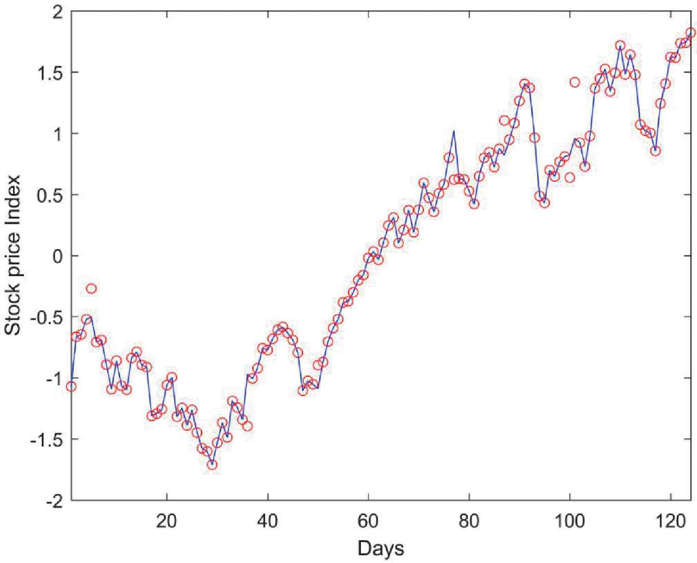
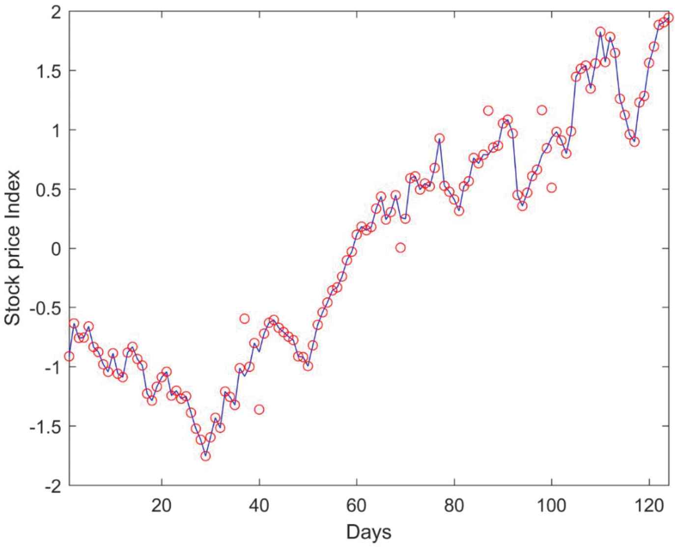
Table 5 presents the quantified performance measures of various NN methods with Nifty 50 dataset. Among all the methods, the proposed RANN model is outperforming with lower error rates of 70.96, 15.56, 0.69 and higher prediction accuracy of 88.50, 76.93, 69.07 with Group-2 input variables. A comparison between a sample of target price and the corresponding predicted stock price from the RANN model with Group-2 variables are depicted in Figure 4. The solid line represents the target price and the red circle markers represent the predicted price. Presenting the prediction results of all the classifiers makes the plot complex, hence it is compared only with the proposed model alone.
| NN Models | Input Variables | RMSE | MAD | MAPE | DA | CP | CD |
|---|---|---|---|---|---|---|---|
| Group-1 | 87.57 | 21.42 | 1.53 | 87.73 | 76.31 | 68.53 | |
| RANN | Group-2 | 70.96 | 15.56 | 0.69 | 88.50 | 76.93 | 69.07 |
| Group-3 | 72.59 | 17.01 | 0.74 | 82.80 | 75.43 | 68.64 | |
| Group-1 | 86.83 | 23.63 | 1.28 | 66.85 | 73.56 | 63.75 | |
| LSTM | Group-2 | 97.73 | 29.26 | 1.98 | 69.57 | 73.43 | 63.64 |
| Group-3 | 84.63 | 22.14 | 1.41 | 85.48 | 74.68 | 64.72 | |
| Group-1 | 102.11 | 29.93 | 1.26 | 81.75 | 74.93 | 64.94 | |
| ELM | Group-2 | 95.31 | 27.26 | 0.90 | 79.76 | 73.56 | 63.75 |
| Group-3 | 100.65 | 29.30 | 0.88 | 71.08 | 73.06 | 63.32 | |
| Group-1 | 92.78 | 27.80 | 1.99 | 80.43 | 72.81 | 63.10 | |
| WNN | Group-2 | 98.04 | 29.20 | 1.85 | 83.81 | 73.81 | 63.97 |
| Group-3 | 104.54 | 32.21 | 0.85 | 61.49 | 72.19 | 62.56 | |
| Group-1 | 110.46 | 36.59 | 1.50 | 75.52 | 72.93 | 63.21 | |
| GA-ANN | Group-2 | 110.12 | 35.92 | 1.85 | 85.85 | 73.68 | 63.86 |
| Group-3 | 108.61 | 36.19 | 1.21 | 80.77 | 72.93 | 63.21 | |
| Group-1 | 125.49 | 46.68 | 1.73 | 80.42 | 74.06 | 64.18 | |
| DNN | Group-2 | 120.55 | 43.44 | 1.81 | 76.69 | 73.31 | 63.53 |
| Group-3 | 122.73 | 45.80 | 0.78 | 67.87 | 74.80 | 64.83 | |
| Group-1 | 124.98 | 44.73 | 2.84 | 69.87 | 74.30 | 64.40 | |
| NN-NLICA | Group-2 | 122.17 | 45.55 | 1.80 | 61.66 | 72.93 | 63.21 |
| Group-3 | 117.63 | 43.04 | 1.08 | 67.21 | 73.18 | 63.43 | |
| Group-1 | 129.34 | 49.87 | 0.94 | 72.20 | 71.93 | 65.80 | |
| RBFNN | Group-2 | 127.14 | 47.92 | 1.81 | 74.15 | 74.55 | 64.61 |
| Group-3 | 129.17 | 50.98 | 2.21 | 71.03 | 72.92 | 66.67 |
Performance comparison of the NN model with Nifty50 dataset.
Target and predicted stock price comparison for Nifty 50 Dataset with repairing artificial neural network (RANN) model.
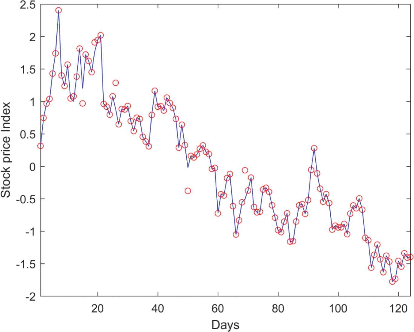
Table 6 list the estimated performance measures of various NN methods with Nifty Bank dataset. Comparatively, the proposed RANN model is outperforming with lower error rates of 70.82, 15.09, 0.23 and higher prediction accuracy of 81.58, 85.43, 73.64 with Group-2 input variables. A comparison between a sample of target price and the corresponding predicted stock price from RANN model with Group-2 variables are depicted in Figure 5.
| NN Models | Input Variables | RMSE | MAD | MAPE | DA | CP | CD |
|---|---|---|---|---|---|---|---|
| RANN | Group-1 | 76.51 | 18.66 | 0.33 | 81.17 | 83.31 | 73.53 |
| Group-2 | 70.82 | 15.09 | 0.23 | 81.58 | 85.43 | 73.64 | |
| Group-3 | 77.95 | 19.72 | 0.27 | 69.12 | 84.68 | 72.99 | |
| Group-1 | 93.16 | 25.65 | 0.41 | 62.12 | 74.18 | 64.29 | |
| LSTM | Group-2 | 91.09 | 25.93 | 0.41 | 59.81 | 73.06 | 63.32 |
| Group-3 | 94.05 | 26.76 | 2.57 | 54.57 | 73.68 | 63.86 | |
| Group-1 | 97.93 | 28.50 | 0.51 | 52.54 | 71.44 | 61.91 | |
| ELM | Group-2 | 102.34 | 29.96 | 0.64 | 54.06 | 73.56 | 63.75 |
| Group-3 | 94.52 | 26.81 | 1.55 | 75.16 | 73.93 | 64.07 | |
| Group-1 | 94.94 | 28.07 | 0.55 | 79.57 | 74.06 | 64.18 | |
| WNN | Group-2 | 97.59 | 29.54 | 2.03 | 75.52 | 72.43 | 62.78 |
| Group-3 | 101.92 | 31.76 | 0.54 | 70.22 | 74.80 | 64.83 | |
| Group-1 | 117.84 | 39.61 | 0.65 | 66.38 | 74.30 | 64.40 | |
| GA-ANN | Group-2 | 114.65 | 37.49 | 1.24 | 68.47 | 72.43 | 62.78 |
| Group-3 | 111.16 | 36.96 | 2.30 | 64.94 | 74.06 | 64.18 | |
| Group-1 | 121.17 | 44.53 | 0.89 | 58.31 | 73.06 | 63.32 | |
| DNN | Group-2 | 123.79 | 45.25 | 0.96 | 74.19 | 73.31 | 63.53 |
| Group-3 | 126.19 | 47.52 | 0.89 | 63.56 | 75.93 | 65.80 | |
| Group-1 | 121.69 | 44.63 | 1.21 | 75.30 | 73.81 | 63.97 | |
| NN-NLICA | Group-2 | 126.60 | 47.47 | 1.06 | 69.22 | 72.93 | 63.21 |
| Group-3 | 124.19 | 46.12 | 1.08 | 67.21 | 74.18 | 64.29 | |
| Group-1 | 129.60 | 50.61 | 1.88 | 53.80 | 73.81 | 63.97 | |
| RBFNN | Group-2 | 122.86 | 47.04 | 2.37 | 74.17 | 75.30 | 65.26 |
| Group-3 | 137.38 | 55.02 | 1.48 | 64.43 | 74.93 | 64.94 |
Performance comparison of the NN model with Nifty-Bank dataset.
Target and predicted stock price comparison for Nifty Bank Dataset with repairing artificial neural network (RANN) model.
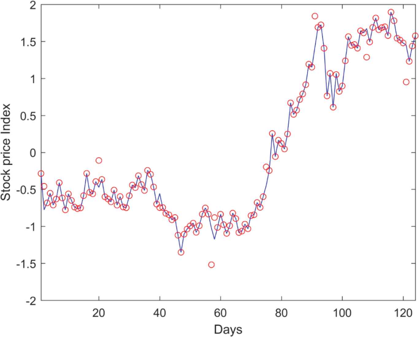
Table 7 presents the estimated performance measures of various NN methods with Nifty Pharma dataset. Comparatively, the proposed RANN model shows a significant performance with lower error rates of 65.39, 13.96, 0.41 and higher prediction accuracy of 89.30, 86.55, 78.56 with Group-2 input variables. A comparison between a sample of target price and the corresponding predicted stock price from RANN model with Group-2 variables are depicted in Figure 6.
| NN Models | Input Variables | RMSE | MAD | MAPE | DA | CP | CD |
|---|---|---|---|---|---|---|---|
| RANN | Group-1 | 87.66 | 21.41 | 0.49 | 87.91 | 81.30 | 76.13 |
| Group-2 | 65.39 | 13.96 | 0.41 | 89.30 | 86.55 | 78.56 | |
| Group-3 | 80.00 | 18.93 | 0.47 | 81.96 | 84.80 | 77.34 | |
| LSTM | Group-1 | 88.23 | 24.01 | 0.53 | 79.45 | 77.17 | 66.88 |
| Group-2 | 89.80 | 25.27 | 0.48 | 82.30 | 77.30 | 66.99 | |
| Group-3 | 93.14 | 25.74 | 0.66 | 77.55 | 75.80 | 65.69 | |
| ELM | Group-1 | 94.31 | 26.50 | 1.93 | 68.98 | 76.92 | 66.67 |
| Group-2 | 92.47 | 26.09 | 0.85 | 80.66 | 76.18 | 66.02 | |
| Group-3 | 90.97 | 25.72 | 1.97 | 64.64 | 78.05 | 67.64 | |
| WNN | Group-1 | 102.44 | 31.52 | 0.79 | 77.31 | 76.30 | 66.13 |
| Group-2 | 98.24 | 29.13 | 0.67 | 60.62 | 78.17 | 67.75 | |
| Group-3 | 102.44 | 31.64 | 0.70 | 61.78 | 79.04 | 68.50 | |
| GA-ANN | Group-1 | 114.33 | 38.70 | 0.86 | 52.83 | 76.80 | 66.56 |
| Group-2 | 106.05 | 34.02 | 0.69 | 81.38 | 78.42 | 67.96 | |
| Group-3 | 111.25 | 37.29 | 0.98 | 52.82 | 76.92 | 66.67 | |
| DNN | Group-1 | 113.84 | 41.07 | 1.59 | 57.13 | 75.55 | 65.48 |
| Group-2 | 119.70 | 43.71 | 1.35 | 78.34 | 78.79 | 68.29 | |
| Group-3 | 128.83 | 48.51 | 2.74 | 80.94 | 76.18 | 66.02 | |
| NN-NLICA | Group-1 | 123.58 | 45.13 | 1.66 | 64.60 | 75.80 | 65.69 |
| Group-2 | 120.25 | 44.53 | 1.55 | 60.21 | 77.42 | 67.10 | |
| Group-3 | 121.61 | 43.96 | 1.72 | 49.62 | 76.05 | 65.91 | |
| RBFNN | Group-1 | 124.03 | 47.16 | 1.58 | 66.10 | 75.93 | 65.80 |
| Group-2 | 130.34 | 50.87 | 2.45 | 60.86 | 76.67 | 66.45 | |
| Group-3 | 135.17 | 53.57 | 2.06 | 66.04 | 78.29 | 67.86 |
Performance comparison of the NN model with Nifty-Pharma dataset.
Target and predicted stock price comparison for Nifty Pharma Dataset with repairing artificial neural network (RANN) model.
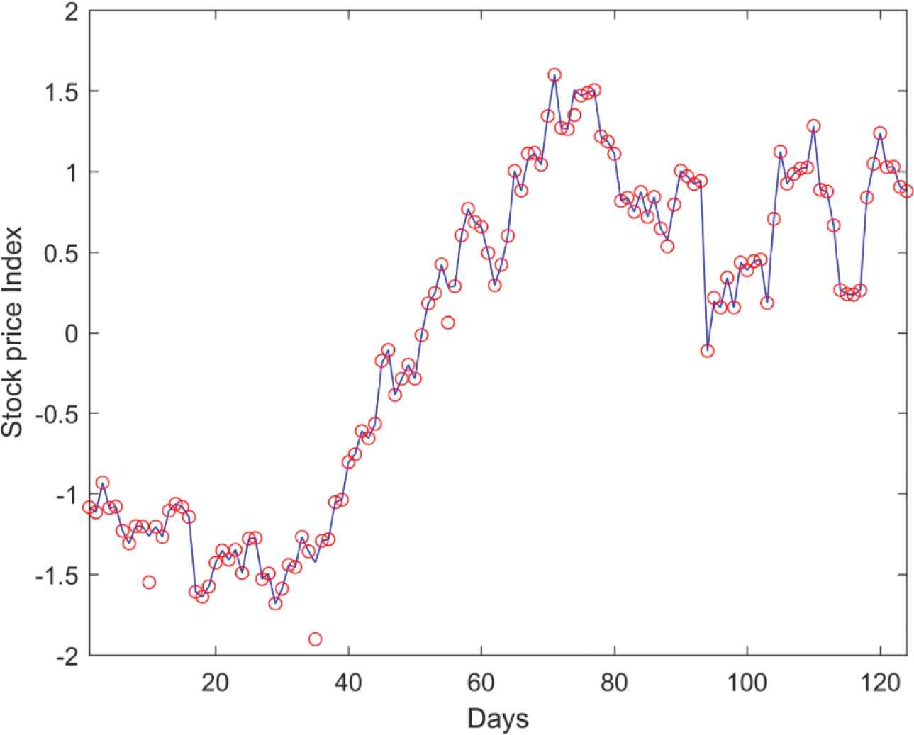
Table 8 list the estimated performance measures of various NN methods with the BSE-IT dataset. Comparatively, the proposed RANN model is outperforming with lower error rates of 61.31, 13.38, 0.26 and higher prediction accuracy of 87.53, 77.93, 74.94 with Group-1 input variables. A comparison between a sample of target price and the corresponding predicted stock price from the RANN model with Group-1 variables are depicted in Figure 7.
| NN Models | Input Variables | RMSE | MAD | MAPE | DA | CP | CD |
|---|---|---|---|---|---|---|---|
| RANN | Group-1 | 61.31 | 13.38 | 0.26 | 87.53 | 77.93 | 74.94 |
| Group-2 | 63.82 | 19.90 | 0.83 | 86.86 | 76.81 | 73.97 | |
| Group-3 | 79.82 | 18.98 | 0.54 | 83.81 | 75.06 | 74.18 | |
| LSTM | Group-1 | 88.65 | 23.82 | 0.39 | 77.94 | 73.81 | 63.97 |
| Group-2 | 99.28 | 28.75 | 1.19 | 71.23 | 74.93 | 64.94 | |
| Group-3 | 96.16 | 26.67 | 0.44 | 59.52 | 74.18 | 64.29 | |
| ELM | Group-1 | 91.19 | 26.38 | 0.41 | 79.70 | 74.68 | 64.72 |
| Group-2 | 100.93 | 29.26 | 0.51 | 81.18 | 75.30 | 65.26 | |
| Group-3 | 92.65 | 26.70 | 1.18 | 75.40 | 73.06 | 63.32 | |
| WNN | Group-1 | 89.95 | 25.87 | 0.46 | 77.09 | 73.81 | 63.97 |
| Group-2 | 107.36 | 32.98 | 1.24 | 80.73 | 73.93 | 64.07 | |
| Group-3 | 104.46 | 32.61 | 0.61 | 63.71 | 74.55 | 64.61 | |
| GA-ANN | Group-1 | 116.01 | 38.91 | 1.17 | 65.83 | 75.68 | 65.59 |
| Group-2 | 109.00 | 35.69 | 0.66 | 73.52 | 72.06 | 62.45 | |
| Group-3 | 113.86 | 38.46 | 1.83 | 60.06 | 73.43 | 63.64 | |
| DNN | Group-1 | 126.47 | 46.52 | 0.96 | 54.49 | 72.68 | 62.99 |
| Group-2 | 116.87 | 41.35 | 0.76 | 71.82 | 74.30 | 64.40 | |
| Group-3 | 122.44 | 46.17 | 1.07 | 80.48 | 72.31 | 62.67 | |
| NN-NLICA | Group-1 | 122.40 | 44.26 | 1.10 | 79.73 | 74.68 | 64.72 |
| Group-2 | 126.22 | 47.57 | 1.38 | 61.78 | 73.81 | 63.97 | |
| Group-3 | 124.12 | 46.09 | 1.30 | 66.11 | 75.05 | 65.05 | |
| RBFNN | Group-1 | 132.30 | 51.69 | 1.33 | 62.20 | 74.55 | 64.61 |
| Group-2 | 136.06 | 53.87 | 1.29 | 60.70 | 73.18 | 63.43 | |
| Group-3 | 129.93 | 50.55 | 1.45 | 67.28 | 74.18 | 64.29 |
Performance comparison of the NN model with BSE-IT dataset.
Target and predicted stock price comparison for BSE IT Dataset with repairing artificial neural network (RANN) model.
Table 9 presents the estimated performance measures of various NN methods with the BSE-Oil and Gas dataset. Comparatively, the proposed RANN model shows a significant performance with lower error rates of 65.01, 13.63, 0.35 and higher prediction accuracy of 85.02, 78.43, 79.64 with Group-2 input variables. A comparison between a sample of target price and the corresponding predicted stock price from the RANN model with Group-2 variables are depicted in Figure 8.
| NN Models | Input Variables | RMSE | MAD | MAPE | DA | CP | CD |
|---|---|---|---|---|---|---|---|
| RANN | Group-1 | 75.38 | 17.72 | 0.36 | 80.36 | 76.93 | 78.07 |
| Group-2 | 65.01 | 13.63 | 0.35 | 85.02 | 78.43 | 79.64 | |
| Group-3 | 82.88 | 20.50 | 0.37 | 84.51 | 74.93 | 75.07 | |
| LSTM | Group-1 | 86.98 | 23.54 | 0.45 | 72.84 | 74.80 | 64.83 |
| Group-2 | 101.34 | 29.74 | 0.69 | 79.45 | 72.93 | 63.21 | |
| Group-3 | 91.58 | 25.31 | 0.54 | 79.26 | 72.43 | 62.78 | |
| ELM | Group-1 | 99.14 | 28.72 | 1.82 | 76.29 | 73.56 | 63.75 |
| Group-2 | 97.53 | 28.29 | 0.75 | 75.35 | 74.06 | 64.18 | |
| Group-3 | 93.41 | 27.45 | 1.47 | 75.34 | 74.30 | 64.40 | |
| WNN | Group-1 | 101.69 | 30.42 | 0.62 | 84.52 | 72.56 | 62.88 |
| Group-2 | 97.40 | 28.87 | 0.60 | 80.76 | 74.68 | 64.72 | |
| Group-3 | 107.75 | 33.70 | 0.60 | 80.64 | 73.43 | 63.64 | |
| GA-ANN | Group-1 | 112.01 | 37.44 | 1.34 | 69.18 | 74.43 | 64.51 |
| Group-2 | 105.69 | 34.46 | 0.65 | 74.94 | 73.06 | 63.32 | |
| Group-3 | 116.07 | 39.82 | 1.40 | 63.28 | 73.31 | 63.53 | |
| DNN | Group-1 | 124.75 | 45.72 | 1.44 | 63.10 | 73.06 | 63.32 |
| Group-2 | 119.88 | 43.19 | 1.85 | 71.70 | 74.93 | 64.94 | |
| Group-3 | 125.07 | 47.15 | 1.41 | 70.44 | 71.81 | 62.24 | |
| NN-NLICA | Group-1 | 121.41 | 45.51 | 1.02 | 78.23 | 72.19 | 62.56 |
| Group-2 | 120.87 | 45.02 | 0.96 | 76.57 | 72.18 | 65.15 | |
| Group-3 | 121.86 | 44.75 | 1.83 | 80.36 | 74.80 | 64.83 | |
| RBFNN | Group-1 | 130.31 | 51.25 | 0.89 | 73.31 | 73.56 | 63.75 |
| Group-2 | 126.68 | 49.93 | 1.17 | 75.18 | 73.18 | 63.43 | |
| Group-3 | 129.44 | 51.04 | 1.22 | 52.50 | 70.94 | 61.48 |
Performance comparison of the NN model with BSE oil & gas dataset.
Target and predicted stock price comparison for BSE Oil & Gas Dataset with repairing artificial neural network (RANN) model.
In addition to comparing the proposed RANN model based prediction with the other models, it is also compared against with the repaired and corrupted data. Table 10 illustrates this comparison between RANN and ANN with unrepaired data (ANNe), the results demonstrates that the unrepaired data achieves lower performance than the repaired one.
| Dataset | NN Models | RMSE | MAD | MAPE | DA | CP | CD |
|---|---|---|---|---|---|---|---|
| Nifty 50 | RANN | 70.96 | 15.56 | 0.69 | 88.50 | 76.93 | 69.07 |
| ANNe | 128.40 | 48.75 | 0.74 | 50.22 | 61.13 | 62.50 | |
| Nifty Bank | RANN | 70.82 | 15.09 | 0.23 | 81.58 | 85.43 | 73.64 |
| ANNe | 133.87 | 50.25 | 1.84 | 63.34 | 79.34 | 69.44 | |
| Nifty Pharma | RANN | 65.39 | 13.96 | 0.41 | 89.30 | 86.55 | 78.56 |
| ANNe | 182.38 | 45.18 | 6.49 | 60.49 | 61.81 | 46.20 | |
| BSE IT | RANN | 61.31 | 13.38 | 0.26 | 87.53 | 77.93 | 74.94 |
| ANNe | 162.44 | 57.75 | 2.83 | 51.87 | 53.18 | 46.79 | |
| BSE Oil & Gas | RANN | 65.01 | 13.63 | 0.35 | 85.02 | 78.43 | 79.64 |
| ANNe | 160.31 | 71.52 | 1.99 | 43.11 | 53.65 | 43.57 |
Performance comparison of prediction model with corrupted and repaired data.
The prediction models are implemented with Matlab R2018® environment, and executed in 64-bit Windows 8.1 operating system, Intel-i5 processor, 8-GB memory configuration. Table 11 presents the comparison study on average computation time taken by each model from 10 trial runs. Comparatively the proposed RANN method achieves better prediction in minimum computation time.
| Computation Time (sec) |
||||||||
|---|---|---|---|---|---|---|---|---|
| Dataset | RANN | LSTM | ELM | WNN | GA-ANN | DNN | NN-NLICA | RBFNN |
| Nifty 50 | 78.12 | 89.05 | 105.21 | 134.01 | 138.20 | 226.10 | 136.55 | 141.08 |
| Nifty Bank | 81.82 | 88.86 | 105.61 | 132.54 | 147.61 | 217.08 | 145.16 | 142.23 |
| Nifty Pharma | 94.78 | 99.96 | 112.39 | 137.29 | 145.27 | 216.68 | 144.83 | 137.87 |
| BSE IT | 94.78 | 102.58 | 110.33 | 136.51 | 145.51 | 219.62 | 160.31 | 128.82 |
| BSE Oil & Gas | 93.61 | 96.49 | 100.13 | 140.32 | 155.03 | 212.47 | 161.91 | 129.79 |
Performance comparison of stock prediction models based on computation cost.
Predicting the stock price with most relevant technical indicators would improve the prediction accuracy, in this way the computation time required by the prediction model could be reduced as the learning is proceeded with minimum inputs [50]. The concept of choosing more relevant input variables is known as feature selection or dimensionality reduction, aims to remove irrelevant or redundant features from a dataset to improve prediction performance. Zhong and Enke [51], applied principal component analysis (PCA) based feature selection methods for feature subset selection in stock forecasting domain. The experimental results indicated that the reduced feature set from PCA with ANN-based classification achieved higher prediction accuracy than with the complete features. Gündüz et al. [52], proposed a feature selection approach using gain ratio and relief function and reported significant performance improvement in stock forecasting. Haq et al. [53], proposed a multi-filter feature selection (MFFS) approach for choosing relevant technical indicators. Three different feature selection methods such as: L1 regularized logistic regression (L1-LR), SVM, and random forest (RF) are applied to rank the technical indicators and the top-ranked indicators are chosen and grouped to form the optimal feature subset. The investigation results shown that the input variables selected from MFFS approach outperforms with greater stock price prediction accuracy than the other approaches.
Here, the technical indicators from all the three groups are combined to form one complete set of 48 features. In preliminary step, one indicator, MA5 from Group-1, two indicators K & D from Group-2 and 5 indicators (LW%R, Disparity in 5 Days, Disparity in 10 Days, OSCP and RSI) from Group-3 are removed from the feature set as they were redundant. With the pre-filtered set of 40 features, the MFFS approach as discussed in Haq et al. [53], is employed to choose the most relevant features. The feature ranking is estimated for all five datasets and found that the ranking is different for each stock dataset. The mean ranking is estimated for each indicator and they are normalized between the range [0, 1]. Once the normalized mean ranking is computed, a threshold value is fixed to drop the features whose ranking are lower than the threshold. For the three approaches, the threshold values 0.03, 0.1 and 0.2 are fixed for L1-LR, SVM and RF respectively. The technical indicators having higher ranking than these threshold values are chosen from all the three feature selection approaches are merged to form the optimal feature subset. MFFS approach results in four subset of features, top-ranked features from three different feature selection approach and the combined subset. Table 12 lists the features selected from MFFS.
| Methods | #Features | Selected Features |
|---|---|---|
| L1-LR | 13 | OBV, ASY5, 5MA, 6MA, 5BIAS, 10BIAS, 12W%R, MACD, 6RSI, 12RSI, Stochastic %K, Stochastic %D, A/D Oscillator |
| SVM | 10 | OBV, 5MA, 6MA, 5BIAS, 10BIAS, MACD, Stochastic %K, Stochastic %D, ROC, CCI |
| RF | 9 | OBV, 5MA, 6MA, 5BIAS, 10BIAS, MACD, Stochastic %K, Stochastic %D, CCI |
| MFFS | 15 | OBV, ASY5, 5MA, 6MA, 5BIAS, 10BIAS, 12W%R, MACD, 6RSI, 12RSI, Stochastic %K, Stochastic %D, A/D Oscillator, ROC, CCI |
Optimal technical indicators identified by feature selection methods.
The stock price prediction performance based on directional accuracy (DA) measure is analyzed with these reduced feature subset and the results are depicted in Table 13. The results indicate that the reduced features from MFFS approach is achieving higher prediction accuracy than the other methods.
| Dataset | Directional Accuracy |
||||
|---|---|---|---|---|---|
| MFFS | RF | SVM | L1-LR | Original | |
| Nifty 50 | 98.37 | 92.87 | 93.28 | 92.30 | 88.50 |
| Nifty Bank | 88.04 | 86.48 | 86.43 | 85.49 | 81.58 |
| Nifty Pharma | 95.20 | 94.07 | 93.97 | 93.25 | 89.30 |
| BSE IT | 92.29 | 91.13 | 91.90 | 90.98 | 87.53 |
| BSE Oil & Gas | 90.35 | 89.30 | 89.26 | 88.49 | 85.02 |
Stock price predication performance analysis on feature selection methods.
7. CONCLUSIONS
The ANN models are proven to be effective for stock price forecasting. However, they are not capable of handling dynamic data updates means that, whenever there is a change in the existing dataset, the learning process has to be repeated once again. Here, a novel NN model, RANN is proposed to adopt the dynamic nature of the dataset. The learning step could be suspended at any point in time, and the dynamic changes like changing attribute values, change of decision labels, removing outdated data samples, removing an attribute, inserting an attribute, could be adapted to the existing learned model. The dynamic changes are adopted by renovating the NN architecture or by adjusting the weights. In this way, it is not required to repeat the complete learning procedure, hence it reduces the computation cost. The performance of the proposed model is validated with five standard stock market datasets such as Nifty 50, Nifty Bank, Nifty Pharma, BSE IT, and BSE Oil and Gas. Five years of data are collected for each dataset, and the stock price forecasting performance is measure with three error rates and three prediction accuracy measures. The RANN model is compared with the existing five different NN models. The investigated results have shown that the RANN model is achieving lower error rates and higher prediction accuracy while adopting dynamic changes. In future, it is planned to explore the other learning models such as deep learning, LSTM, and convolutional neural network for stock price forecasting as well as to contribute toward achieving better prediction rate.
REFERENCES
Cite this article
TY  - JOUR
AU  - S. M. Prabin
AU  - M. S. Thanabal
PY  - 2021
DA  - 2021/04/19
TI  - A Repairing Artificial Neural Network Model-Based Stock Price Prediction
JO  - International Journal of Computational Intelligence Systems
SP  - 1337
EP  - 1355
VL  - 14
IS  - 1
SN  - 1875-6883
UR  - https://doi.org/10.2991/ijcis.d.210409.002
DO  - 10.2991/ijcis.d.210409.002
ID  - Prabin2021
ER  -