International Journal of Computational Intelligence Systems

Volume 14, Issue 1, 2021, Pages 1373 - 1387

Communication-Efficient Distributed SGD with Error-Feedback, Revisited

Authors
Tran Thi Phuong1, 2, 3, *, ORCID, Le Trieu Phong3, ORCID
1Faculty of Mathematics and Statistics, Ton Duc Thang University, No.19 Nguyen Huu Tho Street, Tan Phong Ward, District 7, Ho Chi Minh City, Vietnam
2Meiji University, 1-1-1 Higashi-Mita, Tama-ku, Kawasaki-shi, Kanagawa, 214-8571, Japan
3National Institute of Information and Communications Technology (NICT) 4-2-1, Nukui-Kitamachi, Koganei, Tokyo, 184-8795, Japan
*Corresponding author. Email: tranthiphuong@tdtu.edu.vn
Corresponding Author
Tran Thi Phuong
Received 15 July 2020, Accepted 31 March 2021, Available Online 20 April 2021.
DOI
10.2991/ijcis.d.210412.001How to use a DOI?
Keywords
Optimizer; Distributed learning; SGD; Error-feedback; Deep neural networks
Abstract

We show that the convergence proof of a recent algorithm called dist-EF-SGD for distributed stochastic gradient descent with communication efficiency using error-feedback of Zheng et al., Communication-efficient distributed blockwise momentum SGD with error-feedback, in Advances in Neural Information Processing Systems 32: Annual Conference on Neural Information Processing Systems 2019 (NeurIPS 2019), 2019, pp. 11446–11456, is problematic mathematically. Concretely, the original error bound for arbitrary sequences of learning rate is unfortunately incorrect, leading to an invalidated upper bound in the convergence theorem for the algorithm. As evidences, we explicitly provide several counter-examples, for both convex and nonconvex cases, to show the incorrectness of the error bound. We fix the issue by providing a new error bound and its corresponding proof, leading to a new convergence theorem for the dist-EF-SGD algorithm, and therefore recovering its mathematical analysis.

Copyright
© 2021 The Authors. Published by Atlantis Press B.V.
Open Access
This is an open access article distributed under the CC BY-NC 4.0 license (http://creativecommons.org/licenses/by-nc/4.0/).

1. INTRODUCTION

1.1. Background

For training deep neural networks over large-scale and distributed datasets, distributed stochastic gradient descent (distributed SGD) is a vital method. In distributed SGD, a central server updates the model parameters using information transmitted from distributed workers, as illustrated in Figure 1.

Figure 1

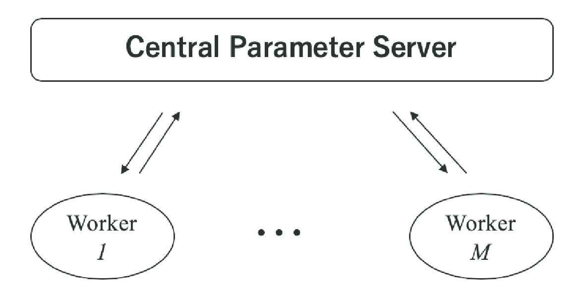
The computation model of distributed SGD. Multiple workers communicate with a central parameter server synchronously. Each worker, after local computations on its data, uploads selected results to the server. The server aggregates all uploaded results from the workers, and sends back the aggregated result from its computations to all workers. These are iterated for multiple rounds.

Communication between the server and distributed workers can be a bottleneck in distributed SGD. Alleviating the bottleneck is a considerable concern of the community, so that variants of distributed SGD using gradient compression have been proposed to reduce the communication cost between workers and the server.

Recently, Zheng et al. [1] proposed an algorithm named dist- EF-SGD recalled in Algorithm 1, in which gradients are compressed before transmission, and errors between real and compressed gradients in one step of the algorithm are re-used in future steps.

1.2. Our Contributions

In this paper, we point out a flaw in the convergence proof of Algorithm 1 given in Zheng et al. [1]. We then fix the flaw by providing a new convergence theorem with a new proof for Algorithm 1.

Zheng et al. [1] stated the following theorem for any sequence of learning rate {ηt}.

Theorem A

(Theorem 1 of [1], problematic). Suppose that Assumptions 1-3 (given together with related notations in Section 2) hold. Assume that the learning rate 0<ηt<32L for all t ⩾ 0. For sequence xt generated from Algorithm 1, we have the following upper bound on the expected Euclidean norm of gradients:

E[f(xo)2]4(f(x0)f)k=0T1ηk(32Lηk)+2Lσ2Mt=0T1ηt2k=0T1ηk(32Lηk)+32L2(1δ)G2δ2[1+16δ2]t=0T1ηtηt12k=0T1ηk(32Lηk)
where o ∈ {0, …, T − 1} is an index such that the probability
Pr(o=k)=ηk(32Lηk)t=0T1ηt(32Lηt),k=0,,T1.

Problem in Theorem A.

Unfortunately, the proof of Theorem A as given in [1] becomes invalidated when the learning rate sequence {ηt} is decreasing. In that proof, a lemma is employed to handle decreasing learning rate sequences. However, in Section 3 we present several counter-examples showing that lemma does not hold. We move on to fix that lemma and finally obtain the following result as our correction for Theorem A.

Theorem 1.

(Our correction for Theorem A) With all notations and assumptions are identical to Theorem A, we have

E[f(xo)2]4(f(x0)f)k=0T1ηk(32Lηk)+2Lσ2Mt=0T1ηt2k=0T1ηk(32Lηk)+8(1δ)(2δ)G2L2δk=0T1ηk(32Lηk)t=0T1ηtηt12k=0t1ηt1k2ηt12αk+16(1δ)(2δ)3G2L2δ2k=0T1ηk(32Lηk)×     t=0T1ηtηt12j=0t1αt1jk=0jηjk2ηt12αk,
where α=1δ2 and o{0,,T1} is an index

Algorithm 1 Distributed SGD with Error-Feedback (dist-EF-SGD) [1]

1: Input: Loss function L, learning rate {ηt} with η1 = 0; number of workers M; compressor C()

2: Initialize: initial parameter x0d; error e0,i=0d on each worker i; error e~0=0d on server

3: for t{0,,T1} do

4:  • on each worker 1 ⩽ iM:

5:    pick data ξt,i from the dataset

6:    gt,i=L(xt,ξt,i) ▷ stochastic gradient

7:    pt,i=gt,i+ηt1ηtet,i ▷ gradient added with previous error

8:    push Δt,i=C(pt,i) to server ▷ gradient compression at worker, and transmission

9:    pull Δ~t from server

10:   xt+1=xtηtΔ~t ▷ local weight update

11:   et+1,i=pt,iΔt,i ▷ local error-feedback to next step

12:  • on central parameter server:

13:   pull ∆t,i from each worker i

14:   p~t=1Mi=1MΔt,i+ηt1ηte~t ▷ gradient average with error

15:   push Δ~t=C(p~t) to each worker ▷ gradient compression at server

16:   e~t+1=p~tΔ~t ▷ error on server

17: end for

such that the probability

Pr(o=k)=ηk(32Lηk)t=0T1ηt(32Lηt),k=0,,T1.

In addition, we show that the upper bound in Theorem 1 becomes O(1MT) for a proper choice of decreasing sequence {ηt} in Corollary 2. Moreover the upper bound in Theorem 1 matches previous results given in Zheng et al. [1] when {ηt} is nondecreasing (Corollary 1).

1.3. Paper Roadmap

We begin with notations and settings in Section 2. In Section 3, we provide counter-examples to justify the issue in [1] for both nonconvex and convex cases. We then correct the issue in Section 4 and then present a proof for Theorem 1 in Section 5.

1.4. Related Works

The use of gradient compression for reducing the communication cost is widely considered in distributed machine learning recently. One line of research is to compress the gradient only on the worker side before sending the result to the parameter server, namely one-side compression. The parameter server receives and aggregates these results and sends back the aggregated result to all workers. Some recent papers such as [25] are in this line of research.

Another line of research uses gradient compression on both workers and server, namely two-side compression. In these two-side compression methods, the workers send the compressed local gradients or some corrected forms of them to the parameter server, and the parameter server compresses the aggregated result before sending it back to all workers. Papers [1,6,7] use two-side compression with an identical method of gradient compression for both workers and the parameter server. Paper [8] considers two-side compression with flexible compression for both workers and the parameter server.

2. PRELIMINARIES

Let , be the inner product of vectors. The Cauchy–Schwarz inequality states that for all vectors u, v it holds that |u,v|2u,u×v,v. The Young inequality γ > 0 (sometimes called the Peter–Paul inequality) states that (a + b)2 ⩽ (1 + γ)a2 + (1 + 1/γ)b2a, b ∈ ℝ. Let be the Euclidean norm of a vector.

For completeness, we recall the algorithm of Zheng et al. [1] in Algorithm 1 and its explanation as follows. At iteration t, the scale ηt1ηt of the local accumulated error vector et,i is added to the gradient gt,i (line 7 of Algorithm 1) for the compression step. Each worker i stores these local accumulated error vector et,i and local corrected gradient vector pt,i for the next iteration. The compressed ∆t,i of pt,i are pushed to the parameter server. The parameter server aggregates these ∆t,i and uses the aggregated result to update the global error-corrected vector p~t (line 14 of Algorithm 1), which in turn is used to update the global accumulated error vector e~t+1 (line 16 of Algorithm 1). Each worker receives the compressed Δ~t of p~t from the parameter server and uses it to update the parameter xt+1.

In order to construct Algorithm 1, Zheng et al. [1] used the idea of Karimireddy et al. [9] that combined gradient compression with error correction. The innovative ideas of Zheng et al. [1] were to apply compression on the parameter server and to use the scale ηt1ηt in line 7 of Algorithm 1. Unfortunately the scale ηt1ηt caused an issue in the proof of convergence theorem of Algorithm 1. We examine this issue in details in Section 3.

2.1. Compressor and Assumptions

Following [5,9], an operator C:dd is a δ-compressor for a number δ(0,1) if

ECC(x)x2(1δ)x2(1)
where the expectation EC is taken over the randomness of C.

Given a loss function , define f(x) = Eξ[(x,ξ)] where xd is the (neural network) model parameters, and ξ is the data batch drawn from some unknown distribution. We consider the following assumptions on f, which are standard and have been used in previous works [1,9].

Assumption 1.

f is lower-bounded, i.e., f* = infxdf(x)<, and L-smooth, i.e., f is differentiable and there exists a constant L ⩾ 0 such that

f(x)f(y)Lxy,x,yd.(2)

By [10], the L-smooth condition in (2) implies that x,yd,

f(x)f(y)+f(y),xy+L2xy2.(3)

Assumption 2.

Let Et denote the expectation at iteration t. Then Et[gt,i] = ∇f(xt) and the stochastic gradient gt,i has bounded gradient, i.e.,

Et[gt,if(xt)2]σ2.

Assumption 3.

The full gradientf is uniformly bounded, i.e., f(xt)2ω2.

Under Assumptions 2 and 3, we have

Et[gt,i2]G2=σ2+ω2,(4)
because Et[gt,if(xt)2]σ2,f(xt)2ω2, and the fact that E[XE[X]2]+E[X]2=E[X2].

2.2. Supporting Lemmas

We need a few supporting lemmas for proving Theorem 1.

Lemma 1.

Let 0<M and xid. Then

1Mi=1Mxi21Mi=1Mxi2.

Proof.

Since xid, xi has the form xi=(xi,1,xi,2,,xi,d)d. We have

1Mi=1Mxi2=1M2i=1Mxi2=1M2(i=1Mxi,1,i=1Mxi,2,,i=1Mxi,d)2=1M2j=1d(i=1Mxi,j)2.

Applying the Cauchy–Schwarz inequality on (i=1Mxi,j)2 gives us

(i=1Mxi,j)2Mi=1Mxi,j2.

Therefore

1Mi=1Mxi21Mj=1d(i=1Mxi,j2)=1Mi=1M(j=1dxi,j2)=1Mi=1Mxi2
which ends the proof.

Lemma 2.

Let {at}, {αt}, {βt} be non-negative sequences insuch that a0 = 0 and, for all t0,

at+1αtat+βt.(5)

Then

at+1βt+j=1ti=jtαiβj1.

In particular, if βt = β for all t, then

at+1β(1+j=1ti=jtαi).

Proof.

By (5), we have

a1α0a0+β0=β0.

Proving by induction, assume that then we have

atβt1+j=1t1i=jt1αiβj1,(6)
then we have
at+1αtat+βt(by (5))βt+αt(βt1+j=1t1i=jt1αiβj1)(by (6))=βt+αtβt1+j=1t1i=jtαiβj1=βt+j=1li=jαiβj1,
which ends the proof.

3. THE ISSUE IN ZHENG ET AL. [1]

In order to prove the convergence theorem for Algorithm 1, Zheng et al. [1] have used the following lemma.

Lemma A

(Lemma 2 of [1], incorrect). For any t0,e~t,et,i,ηt from Algorithm 1, compressor parameter δ at (1), and gradient bound G at (4),

E[e~t+1Mi=1Met,i2]8(1δ)G2δ2(1+16δ2).

Intuitively, Lemma A can become incorrect because its right-hand side only depends on the gradient bound G and compressor parameter δ, and does not capture the scaling factor ηt−1t of the errors e~t and et,i of Algorithm 1. More formally, the following claim states that Lemma A is invalidated when the learning rate sequence {ηt} is decreasing.

Claim 1.

Lemma A (i.e., Lemma 2 of [1]) does not hold. More precisely, referring to Algorithm 1, there exist a sequence of loss functions (xt,ξ), a decreasing sequence {ηt}t1, a number δ with respect to a compressor C, and a step t such that

E[e~t+1Mi=1Met,i2]>8(1δ)G2δ2(1+16δ2).(7)

Claim 1 is justified by the following counter-examples, in which we intentionally utilize the fact that the quotient ηt−1t as in line 7 of Algorithm 1 can be large with decreasing learning rate sequences.

Counter-example 1.

(Convex case) For t ⩾ 0 and xt,ξ, we consider the sequence of loss functions

(xt,ξ)=φ(xt)=14xt
in the constraint set [−1, 1], the decreasing sequence of learning rate {ηt}t1 with
η1=0,{ηt=148t+2}t0,
the compressor C: such that x
C(x)=x0.77.

Then at t = 1, Claim 1 holds true.

Proof.

(Justification of Counter-example 1) It is trivial that the loss function satisfies all the Assumptions 1, 2, and 3. The upper bound gradient of f is G=14 because we have gt,i=14t,i.

  • The function C with C(x)=x0.77 is a compressor with respect to δ = 0.9. Indeed, we have

C(x)x2(1δ)x2x0.77x2(1δ)x210.77121δ.

The last inequality is equivalent to

δ110.7712=0.9107775341541.

Therefore δ = 0.9 suffices.

To continue, let us consider the number of workers is M = 2. Initially e0,i = 0 on each worker i ∈ {1,2} and e~0=0 on server. Because the stochastic gradients are the same on each worker, the results of computations on each worker are the same. So it is sufficient to consider the computations on worker 1 in details.

  • At t = 0 we have the computations on the workers and the server as follows.

    • On worker 1:

      p0,1=g0,1+η1η0e0,1=g0,1=14,Δ0,1=C(p0,1)=p0,10.77=0.3246753246753,e1,1=p0,1Δ0,1=0.07467532467532.

    • On worker 2, p0,2 = p0,1, ∆0,2 = ∆0,1, and e1,2 = e1,1.

    • On server:

      p~0=12(Δ0,1+Δ0,2)+η1η0e~0=Δ0,1=0.3246753246753,Δ~0=C(p~0)=p~00.77=0.42165626581210,e~1=p~0Δ~0=0.09698094113678.

  • At t = 1 we have the computations on the workers and the server as follows:

    • On worker 1:

      p1,1=g1,1+η0η1e1,1=1.6168831168831,Δ1,1=C(p1,1)=p1,10.77=2.0998482037443,e2,1=p1,1Δ1,1=0.48296508686119.

    • On worker 2: p1,2 = p1,1, ∆1,2 = ∆1,1, and e2,2 = e2,1.

    • On server:

      p~1=12(Δ1,1+Δ1,2)+η0η1e~1=Δ1,1+η0η1e~1,=4.52437173216,Δ~1=C(p~1)=p~10.77=5.8758074443687,e~2=p~1Δ~1=1.3514357122048.

Now we compute the left- and right-hand sides of (7) with t = 2.

e~2+12(e2,1+e2,2)2=e~2+e2,12=3.365026291613992
and
8(1δ)G2δ2(1+16δ2)=8(0.1)(14)20.92(1+160.92)=1.2810547172687086.

Thus

e~2+12(e2,1+e2,2)2>8(1δ)G2δ2(1+16δ2),
and then Claim 1 follows.

Counter-example 2.

(Convex case) For t ⩾ 0 and xt,ξ ∈ ℝ, we consider the sequence of loss functions

(xt,ξ)=φ(xt)=xt2
in the constraint set [−1, 1], the decreasing sequence of learning rate {ηt}t⩾−1 with
η1=0,{ηt=34(126t+2)}t0,
and the following compressor C: with parameter δ = 0.9 as in counter-example 1,
C(x)=x0.77.

Then at t = 1, Claim 1 holds true.

Proof.

(Justification of Counter-example 2) It is trivial that the loss function is 2-smooth and satisfies all the Assumptions 1, 2, and 3. Since ∇f(x) = 2x and gt,i=2xt,t,i, we have the upper bound gradient of f in the constraint set [−1, 1] as G = 2. Let us consider the number of workers M = 2. Initially e0,i = 0 on each worker i{1,2} and e~0=0 server. Let us take x0 = 1. Because the stochastic gradients are the same on each worker, the results of computations on each worker are the same. So it is sufficient to consider the computations on worker 1 in details.

  • At t = 0 we have the computations on the workers and the server as follows:

    • On worker 1:

      p0,1=g0,1+η1η0e0,1=g0,1=2,Δ0,1=C(p0,1)=p0,10.77=2.5974025974025974,e1,1=pp0,1Δ0,1=0.5974025974025974.

    • On worker 2, p0,2 = p0,1, ∆0,2 = ∆0,1, and e1,2 = e1,1.

    • On server:

      p~0=12(Δ0,1+Δ0,2)+η1η0e~0=Δ0,1=2.5974025974025974,Δ~0=C(p~0)=p~00.77=3.3732501264968797,x1=x0η0Δ~0=0.26496879743632995,e~1=p~0Δ~0=0.7758475290942823.

  • At t = 1 we have the computations on the workers and the server as follows:

    • On worker 1:

      g1,1=f(x1)=0.5299375948726599,p1,1=g1,1+η0η1e1,1=8.893573958509023,Δ1,1=C(p1,1)=p1,10.77=11.550096050011717,e2,1=p1,1Δ1,1=2.656522091502694.

    • On worker 2, p1,2 = p1,1, ∆1,2 = ∆1,1, and e2,2 = e2,1.

    • On server:

      p~1=12(Δ1,1+Δ1,2)+η0η1e~1=Δ1,1+η0η1e~1=22.41196145733167,Δ~1=C(p~1)=p~10.77=29.106443451080093,e~2=p~1Δ~1=6.694481993748422.

Now we compute the left- and right-hand sides of (7) with t = 2. We have

e~2+12(e2,1+e2,2)2=e~2+e2,12=87.44127740238307
and
8(1δ)G2δ2(1+16δ2)=8(0.1)220.92(1+160.92)=81.98750190519735.

Thus

e~2+12(e2,1+e2,2)2>8(1δ)G2δ2(1+16δ2),
and then Claim 1 follows.

Counter-example 3.

(nonconvex case) For t ⩾ 0,xt ∈ ℝ, we consider the sequence of loss functions

L(xt,ξ)=φ(xt)=11+ext,
the decreasing sequence of learning rate {ηt}t−1 with
η1=0,{ηt=32(148t+2)}t0,
and the following compressor C: with parameter δ = 0.9 as in counter-example 1,
C(x)=x0.77.

Then at t = 1, Claim 1 holds true.

Proof.

(Justification of Counter-example 3) First, we check that Assumptions 1-3 are satisfied.

  • The function ϕ is lower-bounded because 0 ⩽ ϕ(x) ⩽ 1, ∀x ∈ ℝ. The upper bound of ∇ϕ(x) is G=14, since

φ(x)14φ(x)(1φ(x))14φ(x)2+φ(x)140(φ(x)12)20,(8)
which holds true for all x.
  • The function ϕ is L-smooth, with L = 1. Indeed, for all x,y, we have

|φ(x)φ(y)|=|φ(x)(1φ(x))φ(y)(1φ(y))|=|φ(x)φ(y)+(φ(y)φ(x))(φ(y)+φ(x))|=|[φ(x)φ(y)][1(φ(x)+φ(y))]|.

Since 0φ(ξ)1(ξ), we have 0φ(x)+φ(y)2. Therefore 11(φ(x)+φ(y))1, and hence

|[φ(x)φ(y)][1(φ(x)+φ(y))]||φ(x)φ(y)|.

This means that in order to prove |φ(x)φ(y)||xy|, it is sufficient to prove

|φ(x)φ(y)||xy|.(9)

If xy, we obtain ϕ(x) ⩾ ϕ(y). Therefore

(9)φ(x)φ(y)xyφ(x)xφ(y)y

Let φ(x) = ϕ(x)−x. Because ϕ(x)=φ(x)1141<0 by (8), we have φ(x) is a decreasing function. Therefore the inequality φ(x)xφ(y)y holds true, and hence (9) is proven. By the same technique, we obtain (9) for the case x < y.

To continue, let us consider the number of workers M = 2. We initialize e0;i = 0 on each worker i{1,2} and e~0=0 on server. Let us take x0 = 0. Because the stochastic gradients are the same on each worker, the results of computations on each worker are the same. So it is sufficient to consider the computations on worker 1 in details. We have

g0,1=g0,2=φ(x0)=0.25.
  • At t = 0 we have the computations on the workers and the server as follows:

    • On worker 1:

      p0,1=g0,1+η1η0e0,1=g0,1=0.25,Δ0,1=C(p0,1)=p0,10.77=0.3246753246753247,e1,1=p0,1Δ0,1=0.07467532467532467.

    • On worker 2, p0,2 = p0,1, ∆0,2 = ∆0,1, and e1,2 = e1,1.

    • On server:

      p~0=12(Δ0,1+Δ0,2)+η1η0e~0=Δ0,1=0.3246753246753247,Δ~0=C(p~0)=p~00.77=0.42165626581210996,x1=x0η0Δ~0=0.3162421993590825,e~1=p~0Δ~0=0.09698094113678529.

  • At t = 1 we have the computations on the workers and the server as follows.

    • On worker 1:

      g1,1=φ(x1)=0.243852158038919p1,1=g1,1+η0η1e1,1=1.6230309588441978,Δ1,1=C(p1,1)=p1,10.77=2.1078324140833735,e2,1=p1,1Δ1,1=0.4848014552391757.

    • On worker 2, p1,2 = p1,1, ∆1,2 = ∆1,1, and e2,2 = e2,1.

    • On server:

      p~1=12(Δ1,1+Δ1,2)+η0η1e~1=Δ1,1+η0η1e~1=4.532355942503006,Δ~1=C(p~1)=p~10.77=5.886176548705203,e~2=p~1Δ~1=1.3538206062021967.

Now we compute the left- and right-hand sides of (7) with t = 2. We have

e~2+12(e2,1+e2,2)2=e~2+e2,12=3.3805310848189216
and, with δ = 0.9,
8(1δ)G2δ2(1+16δ2)=8(0.1)(14)20.92(1+160.92)=1.2810547172687086.

Thus

e~2+12(e2,1+e2,2)2>8(1δ)G2δ2(1+16δ2),
and hence Claim 1 follows.

4. CORRECTING THE ERROR BOUND OF ZHENG ET AL. [1]

In general, the error E[e~t+1+1Mi=1Met+1,i2] is bounded as follows:

Theorem 2.

(Fix for Lemma 2 of [1]) With e~t,et,i,ηt, and δ from Algorithm 1, for arbitrary {ηt}, we have

E[e~t+1+1Mi=1Met+1,i2]2]2(1δ)(2δ)G2δk=0tηtk2ηt2αk    +4(1δ)(2δ)3G2δ2j=0tαtjk=0jηjk2ηt2αk,
where α=1δ2 and gradient bound G is at (4).

Remark 1.

[Sanity check of the new upper bound] The right-hand side of Theorem 2 can become large together with decreasing leaning rate sequences. Therefore, the error bounds of the sequences in counter-examples 1-3 do satisfy Theorem 2. Indeed, the upper bound on the error in Theorem 2 at t = 1 is

U=2(2δ)(1δ)G2δ(1+η02η12(1δ2))+4(1δ)(2δ)3G2δ2(1+2η02η12(1δ2)).

Concretely, at sanity check,

  • in counter-example 1:

    U=33.550763888888895
    which is indeed larger than
    e~2+1Mi=1Me2,i2=3.365026291613992.

  • in counter-example 2:

    U=675.8530370370372
    which is indeed larger than
    e~2+1Mi=1Me2,i2=87.44127740238307.

  • in counter-example 3:

    U=33.550763888888895
    which is indeed larger than
    e~2+1Mi=1Me2,i2=3.3805310848189216.

Proof.

[Proof of Theorem 2] We have

E[e~t+1+1Mi=1Met+1,i2]2E[e~t+12]+2E[1Mi=1Met+1,i2]2E[e~t+12]+2MiME[et+1,i2],(10)
where the first inequality is by the fact that (a + b)2 ⩽ 2a2 + 2b2,∀a,b, and the second inequality is by Lemma 1. We will separately bound the two terms of (10). Firstly, we consider 1Mi=1ME[et+1,i2]. We have
1Mi=1ME[et+1,i2]=1Mi=1ME[C(pt,i)pt,i2(11)
1δMi=1ME[pt,i2](12)
=1δMi=1ME[gt,i+ηt1ηtet,i2](13)
(1δ)(1+γ)Mi=1ME[ηt1ηtet,i2]+(1δ)(1+1/γ)Mi=1ME[gt,i2](14)
(1δ)(1+γ)ηt12ηt2(1Mi=1ME[et,i2])+(1δ)(1+1/γ)G2,(15)
where (11) and (13) is by the setting of et+1,i and pt,i in Algorithm 1, (12) is by the definition of compressor C, (14) is by Young inequality with any γ > 0, and (15) is by (4). Now, for all t ⩾ 0, applying Lemma 2 to the inequality (15) with
at+1=1Mi=1ME[et+1,i2],αt=(1δ)(1+γ)ηt12ηt2,β=(1δ)(1+1/γ)G2,
we have
1Mi=1ME[et+1,i2]β(1+j=1ti=jtαi)

Moreover, since

1+j=1ti=jtαi=1+j=1ti=jt(1δ)(1+γ)ηi12ηi2=1+j=1tηj12ηt2[(1δ)(1+γ)]t(j1)=j=1t+1ηj12ηt2[(1δ)(1+γ)]t(j1)=k=0tηtk2ηt2[(1δ)(1+γ)]k,
we obtain
1Mi=1ME[et+1,i2](1δ)(1+1/γ)G2k=0tηtk2ηt2[(1δ)(1+γ)]k.

By choosing γ=δ2(1δ), we have

(1δ)(1+1/γ)=(1δ)(2δ)δ
and
(1δ)(1+γ)=1δ2.

Therefore

1Mi=1ME[et+1,i2](2δ)(1δ)G2δk=0tηtk2ηt2αk,(16)
where α=1δ2. Next, we consider the term E[e~t+12] of (10). By the setting of et+1,i and pt,i in Algorithm 1 and the definition of compressor C, we have
E[e~t+12]=E[C(p~t)p~t2](1δ)E[p~t2]=(1δ)E[1Mi=1MC(pt,i)+ηt1ηte~t2](1δ)(1+γ)ηt12ηt2E[e~t2]+(1δ)(1+1/γ)E[1Mi=1MC(pt,i)2],
where the last inequality is by Young inequality for any γ>0. Looking at E[1Mi=1MC(pt,i)2], we have
E[1Mi=1MC(pt,i)2]1Mi=1ME[C(pt,i)2](17)
1Mi=1M(2E[C(pt,i)pt,i2]+2E[pt,i2])(18)
1Mi=1M(2(1δ)E[pt,i2]+2E[pt,i2])=2(2δ)1Mi=1ME[pt,i2],(19)
where (17) is by Lemma 1, (18) is by the fact that (a + b)2 ⩽ 2a2 + 2b2,∀a,b, (19) is by the definition of compressor C. Therefore Moreover, (12) and (16) yield. Therefore
E[e~t+12](1δ)(1+γ)ηt12ηt2E[e~t2]+2(2δ)(1δ)(1+1/γ)1Mi=1ME[pt,i2].

Moreover, (12) and (16) yield

1δMi=1ME[pt,i2](2δ)(1δ)G2δk=0tηtk2ηt2αk.

Therefore

E[e~t+12]

(1δ)(1+γ)ηt12ηt2E[e~t2]+2(2δ)2(1δ)(1+1/γ)G2δk=0tηtk2ηt2αk.

With γ=δ2(1δ), since (1δ)(1+1/γ)=(1δ)(2δ)δ and (1δ)(1+γ)=1δ2=α, we have

E[e~t+12]αηt12ηt2E[e~t2]+2(1δ)(2δ)3G2δ2k=0tηtk2ηt2αk.

By applying Lemma 2 with

at=E[e~i2],αt=αηt12ηt2,βt=2(1δ)(2δ)3G2δ2k=0tηtk2ηt2αk,
we obtain
E[e~t+12]βt+j=1t(i=jtαiβj1).

Since

i=jtαiβj1=i=jtαηi12ηi2βj1=αt(j1)ηj12ηt2βj1,
we have
E[e~t+12]βt+j=1tαt(j1)ηj12ηt2βj1=j=1t+1αt(j1)ηj12ηt2βj1.

Therefore,

E[e~t+12]j=1t+1αt(j1)ηj12ηt22(1δ)(2δ)3G2δ2k=0j1ηj1k2ηj12αk=2(1δ)(2δ)3G2δ2j=1t+1αt(j1)k=0j1ηj1k2ηt2αk=2(1δ)(2δ)3G2δ2j=0tαtjk=0jηjk2ηt2αk.(20)

Substituting (16) and (20) to (10), we obtain

E[e~t+1+1Mi=1Met+1,i2]2(2δ)(1δ)G2δk=0tηtk2ηt2αk  +4(1δ)(2δ)3G2δ2j=0tαtjk=0jηjk2ηt2αk,
as claimed in Theorem 2.

As a sanity check, Theorem 2 matches the results given in [1] when the learning rate is nondecreasing. As a result, Theorems 1 and A agree when the learning rate is nondecreasing.

Corollary 1.

(Sanity check of Theorem 2, cf. Lemma 6 of [1] with μ = 0) In Theorem 2, if {ηt} is a nondecreasing sequence such that ηt>0,t0, then

E[e~t+1+1Mi=1Met+1,i2]8(1δ)G2δ2(1+16δ2).

Proof.

Since {ηt} is nondecreasing, we have ηtk2ηt21. Moreover, since α=1δ2(0,1), we obtain

k=0tηtk2ηt2αkk=0tαk2δ(21)
and
j=0tαtjk=0jηjk2ηt2αkj=0tαtjk=0jαkj=0tαtj(2δ)4δ2.

Replacing (21) and (22) to Theorem 2, we have the result stated in Corollary 1.

5. CORRECTING THE CONVERGENCE THEOREM OF ZHENG ET AL. [1]

Because the error bound plays a crucial role in the proof of the convergence theorem of dis-EF-SGD, fixing [1, Lemma 2] as in Theorem 2 leads to the consequence that the convergence theorem need to be fixed as well.

Proof.

(Proof of Theorem 1) Following [1], we consider the iteration

x~t=xtηt1(e~t+1Mi=1Met,i),
where xt, e~t and et,i are generated from Algorithm 1. Then, by [1, Lemma 1],
x~t+1=x~tηt1Mi=1Mgt,i.(22)

Since f is L-smooth, by (3), we have Moreover, we have

Et[f(x~t+1)]f(x~t)+f(x~t),Et[x~t+1x~t]+L2Et[x~t+1x~t2]=f(x~t)ηtf(x~t),Et[1Mi=1Mgt,i]+Lηt22Ef[1Mi=1Mgt,i2],(23)

Moreover, we have

Et[1Mi=1Mgt,i2]=f(xt)2+Et[1Mi=1Mgt,if(xt)2],(24)
which follows from the fact that E[XE[X]2]=E[X2]E[X]2. Substituting (24) to (23), we obtain
Et[f(x~t+1)]f(x~t)ηtf(x~t),f(xt)   +Lηt22f(xt)2   +Lηt22Et[1Mi=1Mgt,if(xt)2].(25)

Following [1], we assume that {gt,if(xt)}1iM are independent random vectors. Then the assumption Et[gt,i]=f(xt) of Assumption 2 implies that gt,if (xt) are random vectors with 0 means. Therefore

Et[i=1M(gt,if(xt))2]=i=1MEt[gt,if(xt)2]
and hence we have
Et[1Mi=1Mgt,if(xt)2]=Et[1Mi=1M(gt,if(xt))2]=1M2Et[i=1M(gt,if(xt))2]=1M2i=1MEt[gt,if(xt)2]σ2MM2=σ2M.

Substituting the above bound to (25) gives us

Et[f(x~t+1)]f(x~t)ηtf(x~t),f(xt)+Lηt22f(xt)2+Lηt2σ22M.(26)

Moreover, we have

ηtf(x~t),f(xt)=ηtf(xt)f(x~t),f(xt)ηtf(xt),f(xt)=ηtf(xt)f(x~t),f(xt)ηtf(xt)ηtρ2f(xt)2+ηt2ρf(xt)f(x~t)2    ηtf(xt)2(27)
ηt(1ρ2)f(xt)2+ηtL22ρxtx~t2,(28)
where (27) is by the fact that 〈a,b〉 ≤ (ρ/2) ‖a‖ 2 + (ρ1/2)‖b2 for all a,b and real number ρ > 0, and (28) is by Assumption 1. Replacing (28) to (26) gives us
Et[f(x~t+1)]f(x~l)ηt(1Lηt+ρ2)f(xl)2+ηtL22ρxtx~t2+Lηt2σ22M.

Taking ρ=12, we have

Et[f(x~t+1)]f(x~t)ηt(34Lηt2)f(xt)2+ηtL2xtx~t2+Lηt2σ22M.(29)

Since xtx~t=ηt1(e~t+1Mi=1Met,i) by (22), after rearranging the terms and taking total expectation, we obtain

ηt(34Lηt2)E[f(xt)2]    E[f(x~t)f(x~t+1)]+Lηt2σ22M             +ηtηt12L2E[e~t+1Mi=1Met,i2].

Applying Theorem 2 gives us

ηt(34Lηt2)E[f(xt)2](30)
E[f(x~t)f(x~t+1)]+Lηt2σ22M+ηtηt122(2δ)(1δ)G2L2δk=0t1ηt1k2ηt12αk+ηtηt124(1δ)(2δ)3G2L2δ2j=0t1αt1jk=0jηjk2ηt12αk,
where α=1δ2. Since ηt<32L,t, we have
k=0T1ηk4(32Lηk)>0.

Taking summation and dividing by k=0T1ηk4(32Lηk), (30) yields

t=0T1ηt(32Lηt)E[f(xt)2]k=0T1ηk(32Lηk)4(f(x0)f)k=0T1ηk(32Lηk)+2Lσ2Mt=0T1ηt2k=0T1ηk(32Lηk)+8(2δ)(1δ)G2L2δk=0T1ηk(32Lηk)t=0T1ηtηt12k=0t1ηt1k2ηt12αk+16(1δ)(2δ)3G2L2δ2k=0T1ηk(32Lηk)×t=0T1ηtηt12j=0t1αt1jk=0jηjk2ηt12αk.

Following Zheng et al. [1], let o ∈ {0, …, T − 1} be an index such that

Pr(o=k)=ηk(32Lηk)t0T1ηt(32Lηt)

Then

E[f(xo)2]=1k=0T1ηk(32Lηk)t=0T1ηt(32Lηt)E[f(xt)2]
and we obtain the result stated in Theorem 1

The following corollary establishes the convergence rate O(1MT) of Algorithm 1 when the learning rate is decreasing.

Corollary 2.

(Convergence rate with decreasing learning rate) Under the assumptions of Theorem 1, if {ηt} is a decreasing sequence such that

ηt=1((t+1)T)1/4M+T1/3
with sufficiently large T. Then
E[f(xo)2]  2(1MT+1T2/3)[f(x0)f+Lσ2+4(1δ)(2δ)G2L2δ2(1+4δ2),
which yields E[f(xo)2]O(1MT).

Proof.

Following [1], assume that T16L4M2, we have

ηt=1((t+1)T)1/4M+T1/3M((t+1)T)1/4M(t+1)1/4(16L4M2)1/4=1(t+1)1/42L12L.

Therefore ηt<32Lt0, which satisfies the assumption of Theorem 1 on {ηt}. Recall that by Theorem 1, we have

E[f(xo)2]4(f(x0)f)k=0T1ηk(32Lηk)+2Lσ2Mk=0T1ηk(32Lηk)t=0T1ηt2+8(1δ)(2δ)G2L2δk=0T1ηk(32Lηk)t=0T1ηtηt12k=0t1ηt1k2ηt12αk+16(1δ)(2δ)3G2L2δ2k=0T1ηk(32Lηk)×    t=0T1ηtηt12j=0t1αt1jk=0jηjk2ηt12αk,(31)
where α=1δ2 and o{0,,T1} is an index such that
Pr(o=k)=ηk(32Lηk)k=0T1ηt(32Lηt),k=0,,T1.

Since

32Lηt31(t+1)1/42,
we have
1k=0T1ηt(32Lηt)12k=0T1ηt.(32)

Moreover, we have

ηtηt12k=0t1ηt1k2ηt12αk=k=0t1ηtηt1k2αk(33)
and
ηtηt12j=0t1αt1jk=0jηjk2ηt12αk     =j=0t1αt1jk=0jηtηjk2αk.(34)

Substituting (32), (33), and (34) to (31) gives us

E[f(xo)2]2(f(x0)f)t=0T1ηt+Lσ2Mt=0T1ηtt=0T1ηt2  +4(1δ)(2δ)G2L2δt=0T1ηtt=0T1k=0t1ηtηt1k2αk  +8(1δ)(2δ)3G2L2δ2t=0T1ηt×    t=0T1j=0t1αt1jk=0jηtηjk2αk,(35)

Because

ηtηt1k2ηt1k3=1(((tk)T)1/4M+T1/3)31(T1/3)3=1T(36)
and
k=0t1αkk0αk=11α=2δ,(37)
we obtain
t=0T1k=0t1ηtηt1k2αk1Tt=0T1k=0t1αk1Tt=0T12δ=2δ.

By the same reason as in (36) and (37), we have ηtηjk21T, j=0t1αt1j2δ, and k=0jαk2δ. Therefore

t=0T1j=0t1αt1jk=0jηtηjk2αk   1Tt=0T1j=0t1αt1jk=0jαk   1Tt=0T1j=0t1αt1j(2δ)    1Tt=0T14δ2=4δ2.

Moreover, we have

t=0T1ηt2=t=0T11(((t+1)T)1/4M+T1/3)2t=0T11(((t+1)T)1/4M)2=t=0T1M[(t+1)T]1/2=MTt=1T1t2M,
where the last inequality is by the fact that t=1T1t2T. Therefore
E[f(xo)2]2(f(x0)f)t=0T1ηt+2Lσ2t=0T1ηt+8(1δ)(2δ)G2L2δ2t=0T1ηt+32(1δ)(2δ)3G2L2δ4t=0T1ηt.

Furthermore, becauce

t=0T1ηt=t=0T11((t+1)T)1/4(M)+T1/3t=0T11TM+T1/3=11MT+T2/3,
we obtain
1t=0T1ηt1MT+1T2/3.

Therefore

E[f(xo)2]         2(1MT+1T2/3)f(x0)f+Lσ2             +4(1δ)(2δ)G2L2δ2(1+4δ2)
and hence Corollary 2 follows.

6. CONCLUSION

We show that the convergence proof of dist-EF-SGD of Zheng et al. [1] is problematic when the sequence of learning rate is decreasing. We explicitly provide counter-examples with certain decreasing sequences of learning rate to show the issue in the proof of Zheng et al. [1]. We fix the issue by providing a new error bound and a new convergence theorem for the dist-EF-SGD algorithm, which helps recover its mathematical foundation.

CONFLICTS OF INTEREST

The authors declare that there are no conflicts of interest.

AUTHORS' CONTRIBUTIONS

Tran Thi Phuong established the research direction. Both authors contributed to the technical contents, and to the edition of the manuscript. Both authors read, revised, and approved the final manuscript.

ACKNOWLEDGMENTS

We are grateful to Shuai Zheng for his communication and verification. We also thank the anonymous reviewers for their careful comments. The work of Le Trieu Phong was supported in part by JST CREST under Grant JPMJCR19F6.

REFERENCES

1.S. Zheng, Z. Huang, and J.T. Kwok, Communication-efficient distributed blockwise momentum SGD with error-feedback, in Advances in Neural Information Processing Systems 32: Annual Conference on Neural Information Processing Systems (NeurIPS 2019) (Vancouver, Canada), 2019, pp. 11446-11456. https://arxiv.org/abs/1905.10936
2.J. Bernstein, J. Zhao, K. Azizzade-nesheli, and A. Anandkumar, signSGD with majority vote is communication efficient and fault tolerant, in 7th International Conference on Learning Representations (ICLR 2019) (New Orleans, LA, USA), 2019.
3.D. Basu, D. Data, C. Karakus, and S.N. Diggavi, Qsparse-local-SGD: distributed SGD with quantization, sparsification and local computations, in Advances in Neural Information Processing Systems 32: Annual Conference on Neural Information Processing Systems (NeurIPS 2019) (Vancouver, Canada), 2019, pp. 14668-14679.
4.T. Vogels, S.P. Karimireddy, and M. Jaggi, PowerSGD: practical low-rank gradient compression for distributed optimization, Curran Associates, Inc, in Advances in Neural Information Processing Systems (Vancouver, Canada), 2019, pp. 14236-14245.
5.S.U. Stich, J.-B. Cordonnier, and M. Jaggi, Sparsified SGD with memory, in Advances in Neural Information Processing Systems 31: Annual Conference on Neural Information Processing Systems (Montréal, Canada), 2018, pp. 4452-4463.
6.H. Tang, C. Yu, X. Lian, T. Zhang, and J. Liu, DoubleSqueeze: parallel stochastic gradient descent with double-pass error-compensated compression, K. Chaudhuri and R. Salakhutdinov (editors), Proceedings of the 36th International Conference on Machine Learning, vol. 97 of Proceedings of Machine Learning Research (PMLR), PMLR, Long Beach, California, USA, 2019, pp. 6155-6165.
7.X. Liu, Y. Li, J. Tang, and M. Yan, A double residual compression algorithm for efficient distributed learning, in Proceedings of Machine Learning Research (PMLR) (Palermo, Italy), 2020, pp. 133-143.
9.S.P. Karimireddy, Q. Rebjock, S.U. Stich, and M. Jaggi, Error feedback fixes signSGD and other gradient compression schemes, in Proceedings of the 36th International Conference on Machine Learning (ICML 2019) (Long Beach, California, USA), 2019, pp. 3252-3261. https://arxiv.org/abs/1901.09847
Journal
International Journal of Computational Intelligence Systems
Volume-Issue
14 - 1
Pages
1373 - 1387
Publication Date
2021/04/20
ISSN (Online)
1875-6883
ISSN (Print)
1875-6891
DOI
10.2991/ijcis.d.210412.001How to use a DOI?
Copyright
© 2021 The Authors. Published by Atlantis Press B.V.
Open Access
This is an open access article distributed under the CC BY-NC 4.0 license (http://creativecommons.org/licenses/by-nc/4.0/).

Cite this article

TY  - JOUR
AU  - Tran Thi Phuong
AU  - Le Trieu Phong
PY  - 2021
DA  - 2021/04/20
TI  - Communication-Efficient Distributed SGD with Error-Feedback, Revisited
JO  - International Journal of Computational Intelligence Systems
SP  - 1373
EP  - 1387
VL  - 14
IS  - 1
SN  - 1875-6883
UR  - https://doi.org/10.2991/ijcis.d.210412.001
DO  - 10.2991/ijcis.d.210412.001
ID  - Phuong2021
ER  -