
Analytical Reduction Method for New Type-2 Fuzzy Chance-Constrained Portfolio Selection Model
 , Jindong Qin2, Xinwang Liu3, Xu Zhang1,
 - DOI
- 10.2991/ijcis.d.210507.001How to use a DOI?
- Keywords
- Type-2 fuzzy return; Analytical reduction method; Portfolio selection; Credibility measure
- Abstract
In the traditional portfolio selection problem, asset returns are modeled as fuzzy variables with fuzzy return. However, this approach is limited in its ability to capture uncertainty accurately and in analytical model solving. Here, we aim to develop a new fuzzy chance-constrained portfolio model with a type-2 fuzzy return variable using a credibility measure. In real practice, an effective portfolio model under a new, more complex environment is required to improve instinctive imprecision. Here, we propose a novel analytical reduction method to transform our proposed model into a linear programing model with linear constraints, and use a linear programing tool to obtain optimal portfolio strategies. We first reformulate the portfolio model with type-2 fuzzy returns using two types of chance criteria. Next, we provide a new analytical method to solve the proposed model. Then, we present a numerical example with 20 asset returns described by a triangular membership function and use comparison testing to illustrate the advantages of our proposed method. The numerical results show that the relationship between investor tolerance of portfolio risk and the values attained for the four objective functions is in line with our expectations regarding the risk–return trade-off, and the comparison test results indicate that our proposed reduction method performs better than three existing methods. Our method provides an effective practice model for reformulating type-2 fuzzy portfolio problems using an analytical reduction method. Although a large number of existing type-2 fuzzy portfolio problems cannot be solved by our analytical method, it represents a new tool to solve these kinds of problems.
- Copyright
- © 2021 The Authors. Published by Atlantis Press B.V.
- Open Access
- This is an open access article distributed under the CC BY-NC 4.0 license (http://creativecommons.org/licenses/by-nc/4.0/).
1. INTRODUCTION
The portfolio selection problem involves selecting an optimal combination of financial assets to maximize the investor’s expected return. This problem dates back to the original work of Markowitz [1] on the mean–variance model for the trade-off between risk and return. Returns of individual securities are generally assumed to be random variables. By contrast, asset returns are sometimes modeled as fuzzy variables rather than stochastic variables because of the potential existence of multi-fold uncertainty. In particular, owing to instinctive imprecision, it is not easy to estimate the membership degree of a fuzzy demand. To overcome those difficulties, Wu et al. [2] proposed five constrained uncertainty measures (centroid, cardinality, fuzziness, variance, and skewness) for well-shaped interval type-2 fuzzy sets (IT2FSs) using the constrained representation theorem, in order to capture uncertainty more precisely. In fact, type-1 fuzzy sets (T1FSs) are crisp and have two-dimensional membership functions, whereas IT2FSs have three-dimensional membership functions that can better express the uncertainty and the fuzziness of real-world scenarios. Therefore, type-2 fuzzy set theory has advantages over other logic theories [3]. A type-2 fuzzy logic system (T2FLS) allows for a better uncertainty model than does a T1FLS, these studies in Refs. [4,5] state that a type-2 fuzzy set (T2FS) has a footprint of uncertainty that gives it more degrees of freedom than a T1FS. An extension of a traditional T1FS, an IT2FS is a simplified version of a general T2FS, because the membership grade is a crisp interval rather than a function. An IT2FS is defined in the same way as an interval-valued fuzzy set; both of these set types were introduced by Zadeh [6]. IT2FLSs can outperform their T1FLS counterparts in a variety of fields, including information processing [7–9], fuzzy control, and decision-making [10–13].
Although it is difficult to obtain potential risk measures that follow the five axioms, researchers seeking suitable measures for capturing portfolio risk in practice have developed a variety of extended models to quantify risk by semi-variance or variance [14–19]. In reality, although some individuals are sensitive to a preset disastrous loss level and treat the potential probability of it occurring as a risk, others consider all possible loss levels and their probabilities. When investors make a decision to avoid or seek risk, they usually weigh the severity of every potential loss as well as its probability. Therefore, we align ourselves here with these practices.
A significant body of literature describes the use of possibility measures to construct portfolio selection problems, assuming that the returns are fuzzy variables [20–25]. Although possibility measures are useful tools to solve these problems and have been widely used, they have certain weaknesses. For instance, a fuzzy event with a maximum possibility of unity may not occur. Another flaw is that two fuzzy events with different chances of occurrence may have the same possibility value. This is because the possibility measure is not self-dual, which is an important property both in theory and in practice. Therefore, Liu and Yian-Kui [26] proposed a credibility measure to overcome the above limitations inherent in possibility measures. Many other scholars later developed extended fuzzy portfolio selection models based on credibility measures [27–30].
Chance-constrained programing, a method of developing credibilistic models, was first introduced by Charnes and Cooper [31]. Liu [32] developed many general forms of fuzzy chance-constrained programing. The robustness of the chance-constrained method means it is well-suited to solving optimization problems [33–36]. Chance-constrained optimization is widely used in energy management [37–41], risk management [42–45], supply-chain management [46–48], etc. Much research in the area focuses on solving nonlinear dynamic questions with chance constraints [49–52]. However, these problems can be extremely difficult to solve. Probability density functions are often difficult to formulate, especially for nonlinear problems. Moreover, issues with convexity and stability mean that small deviations from the actual density function could cause major changes to the optimal solution. Further complications arise when variables with and without uncertainty cannot be decoupled. Owing to these complications, no single approach exists for solving chance-constrained problems. However, the most common approach to simple questions is to transform the chance constraints into deterministic functions by decoupling the variables with and without uncertainty.
A number of studies have focused on related fuzzy portfolio problems using risk measures. In this way, Huang [53] introduced a fuzzy portfolio selection model. To integrate both a genetic algorithm and the fuzzy simulation for solving their proposed models, they first proposed two types of portfolio chance-constrained models with fuzzy variables, and then designed a new hybrid intelligent algorithm to implement their solution. Recently Mohagheghi et al. [54] formulateda fuzzy portfolio model from a risk-averse perspective, which was shown to be a zero-one integer programing model; specifically, they used a new transformation method that could convert the fuzzy portfolio choice model into an easy crispmathematical model based on qualitative possibility theory. Using ITFS Pai [55] presented a tripartite-stage fuzzy portfolio optimization problem, which included market scenario forecasting and portfolio-rebalancing-based metaheuristics. Coupland and John [56] proposed a new faster technique based on geometric representations and operations for defuzzying aT2FS. Bai and Liu [57] proposed a new type-2 reduction method and established some useful analytical expressions for mean values and second-order moments of common reduced fuzzy variables. Kundu et al. [58] presented the nearest-interval approximation, which was applied to a multi-item solid transportation problem with type-2 fuzzy parameters for continuous type-2 fuzzy variables. Kundu et al. [59] proposed a method to solve linear programing problems with constraints involving interval type-2 fuzzy variables, and successfully used it to solve a solid transportation problem with availabilities, demands, and conveyance capacities as represented by trapezoidal IT2FVs.
From the perspective of chance-constrained multi-objective programing, Mehlawat and Gupta [30] considered a portfolio selection problem with fuzzy parameters. Using the Sharpe ratio and value-at-risk ratio of a portfolio as objectives, Kar et al. [60] reformulated a new bi-objective fuzzy portfolio selection model and further solved it using multi-objective and nondominated sorting genetic algorithms. Inspired by a fuzzy multi-period portfolio selection problem, Guo et al. [61] proposed a mean–variance model with V-shaped transaction costs using credibility theory, and designed a genetic algorithm to solve the proposed model. Kar et al. [62] proposed a multi-objective portfolio selection model by defining average return as expected value, risk as variance, and divergence among security returns as cross-entropy; this model was solved using the Nondominated Sorting Genetic Algorithm II and Archive-Based hybrid Scatter Search. To increase the visibility/differentiating impact of the current issue, we summarize the salient features of the relevant methods in Table 1. Besides the work mentioned above, researchers have employed fuzzy nonlinear modeling approaches in various applications [63–67].
| Author(s) | Uncertain Variable | Method | Measure |
|---|---|---|---|
| Huang [53] | Type-1 | Genetic algorithm | Credibility |
| Huang [68] | Type-1 | Hybrid intelligent algorithm | Credibility |
| Kar et al. [62] | Type-1 | Genetic algorithm | Cross-entropy |
| Mohagheghi et al. [54] | Type-2 | Zero-one integer programing | None |
| Bai and Liu [57] | Type-2 | Defuzzification method | CVAR |
| Coupland and John [56] | Type-2 | Faster geometric method | None |
| Pai [55] | ITFS | Metaheuristics | DR and ER |
| Kundu et al. [58] | Continuous type-2 | Nearest-interval approximation | Generalized credibility |
| Mehlawat and Gupta [30] | Type-1 | Multi-objective programing | Risk curve with credibility |
| Kar et al. [60] | Type-1 | Volutionary algorithms | Sharpe and value-at-risk ratio |
| Kundu et al. [59] | IT2FS | CCP method | Generalized credibility |
| This paper | Type-2 | Analytical reduction method | Risk curve with credibility |
Note: DR and ER denote diversification ratio and expected return, respectively.
Comparison of the proposed model with those in the existing literature.
Owing to different methods structures comparing with the existing methods [including analytical hierarchy process (AHP), Technique for Order Preference by Similarity to an Ideal Solution (TOPSIS), hybrid intelligent algorithm (HIA), and genetic algorithm (GA)], our main idea is concluded as three steps, the first step is reformulating a new type-2 fuzzy portfolio selection model based on credibility measure, and then using the derived proposition, our proposed model is transformed into an easy linear programing model, finally we use the six-step algorithm to obtain the optimal portfolio strategies. Motivated by the limitations of existing work, we attempt to answer the following research questions. How can the portfolio selection model be reformulated under a new type-2 fuzzy environment? How can the proposed type-2 fuzzy portfolio model be solved using an analytical reduction method? What are the advantages of our proposed model compared with those of other methods? We are able to give clear answers to these questions. For fuzzy chance-constrained portfolio choice problems with type-2 fuzzy return variables, our contributions can be summarized as follows:
As T2FSs have advantages over T1FSs, we were particularly interested in how to reformulate the portfolio selection model under a type-2 fuzzy environment; using credibility theory, we reformulate a new type-2 fuzzy chance-constrained portfolio selection model.
In contrast to the existing methods for solving the complexity of a fuzzy portfolio model, we propose a novel analytical reduction method to transform our proposed model into a linear programing model with linear constraints, and further use a linear programing tool to obtain optimal portfolio strategies.
Our proposed novel reduction method for the new model outperforms other methods, including AHP, TOPSIS, HIA, and GA; comparison testing and a numerical example with 20 asset returns described by a triangular membership function confirm the validity of the proposed model and further demonstrate its applications and efficiency.
This paper is organized as follows. Section 2 outlines the fundamentals of credibility, some basic concepts of T2FSs, and the risk curve and confidence curve. Section 3 presents some propositions that have key roles in the subsequent section. In Sections 4 and 5, we formulate the portfolio selection problem and solve the proposed model using the propositions given in Section 3. Section 6 presents comparison testing and an example to illustrate the effectiveness and validity of the proposed model. Finally, Section 7 summarizes the work, draws some conclusions, and presents possible applications.
2. PRELIMINARIES
This section presents various concepts regarding T2FSs, fundamentals of credibility, and risk curves and confidence curves. Furthermore, propositions are introduced to better understand the modeling ideas used in the next section.
2.1. Type-2 Fuzzy Sets
A T2FS denoted by A in X is defined as in Eq. (1) and characterized by a type-2 membership function
A can also be expressed in the following form:
Note that each x has a primary membership function Jx weighted by a secondary membership function.
2.2. Fundamentals of Credibility Fundamentals
Credibility theory [69] is a branch of mathematics that introduces credibility measures, which can be used to better study the behavior of fuzzy events. A credibility measure should follow five axioms that ensure that it has certain mathematical properties.
Cr{π} = 1, which means that the credibility measure of any nonempty set equals 1.
If A ⊆ B, then Cr{A} ⩽ Cr{B}; that is, the credibility measure is nondecreasing.
For any event A ∈ P(π), Cr{A} + Cr{Ac} = 1. This is interpreted as the credibility measure being self-dual.
Cr{∪Ai} ∧ 0.5 = supiCr{Ai} for ∀Aiwith Cr{Ai} ⩽ 0.5.
Let π1, π2,…, πn be the nonempty sets for which Cr1, Cr2,…, Crn satisfy the above four axioms, and let π = π1 × π2 × · · · × πn. Then, Cr{θ1, θ2,…, θn} = Cr{θ1} ∧ Cr{θ2} ∧ · · · ∧ Cr{θn} for each π ∈ (π1, π2,…, πn).
Here, ∧ is a minimal operator and π is a nonempty set; P(π) is the power set of π (i.e., the collection of all subsets of π); and each element in P(π) is called an event. Note that the credibility measure of the empty set is always 0, i.e., Cr{∅}= 0, and it takes values on the interval [0, 1]. A fuzzy variable is usually characterized by a membership function; it is essentially a random variable that is defined as a measurable function on a probability space. Liu [69] defined a fuzzy variable as a function on a credibility space.
To increase the consistency and readability of our proposed model, we provide some basic definitions (see Ref. [69]) as follows.
Definition 1.
Suppose ξ is a general fuzzy variable with membership function μ. The generalized credibility measure
If ξ is normalized, it is easy to check that
Definition 2.
The general fuzzy variables
Definition 3.
Let ξ be a normal fuzzy variable; then, the expected value E[ξ] of ξ is defined as
Definition 4.
Similar to the α-optimistic value of the normalized fuzzy variable, the α-optimistic value of general fuzzy variables can be defined through a generalized credibility measure. Let ξ be a fuzzy variable (not necessarily normalized). Then,
2.3. Risk Curve and Confidence Curve
Definition 5.
[53] Let ξ represent the fuzzy return of the portfolio, and let b represent the target return. The risk curve is then expressed as
Definition 6.
Similar to the risk curve (see Ref. [53]), let ξ be the fuzzy return of the portfolio and let β(r) represent the investor’s confidence curve. Then the portfolio can be defined as safe, in that the risk curve of the portfolio is completely below the investor’s confidence curve:
Definition 7.
[70] The l∞ risk function is defined as
3. MAIN PROPOSITIONS
In this section, we focus on some propositions associated with T2FVs, which play an essential part in solving the proposed model. The main results are reported in the subsequent sections.
Lemma 1.
[71] Let ξ be a type-2 triangular fuzzy variable defined as
Using the optimistic CV reduction method, the reduction ξ1 of
Using the pessimistic CV reduction method, the reduction ξ2 of
Using the CV reduction method, the reduction ξ3 of
Proof.
See the proof of Theorem 4 of [71]. We only prove assertion (i). The remaining assertions can be proved similarly. Note that the secondary possibility distribution
Lemma 2.
[71] Let ξi be the reduction of the type-2 triangular fuzzy variable
Given the generalized credibility level a α ∈ [0, 0.5], if α ∈ [0, 0.25], then
and if α ∈ [0.25, 0.5], thenGiven the generalized credibility level α ∈ [0.5, 1], if α ∈ [0.5, 0.75], then
and if α ∈ [0.75, 1], then
Proof.
The proof refers to Theorem 7 of [71].
Lemma 3.
From Lemma 2, the equivalent expressions of
Based on Lemmas 1 and 2, the following propositions can be obtained.
Proposition 1.
Let
Given the generalized credibility level α ∈ [0, 0.5], if α ∈ [0, 0.25], then
and if α ∈ [0.25, 0.5], thenGiven the generalized credibility level α ∈ [0.5, 1], if α ∈ [0.5, 0.75], then
and if α ∈ [0.75, 1], then
Proposition 2.
Let ζi be the reduction of the type-2 triangular fuzzy variable
Given the generalized credibility risk level β(r) ∈ [0, 0.5], if β(r) ∈ [0, 0.25], then
and if β(r) ∈ [0.25, 0.5], thenGiven the generalized credibility risk level β(r) ∈ [0.5, 1], if β(r) ∈ [0.5, 0.75], then
and if β(r) ∈ [0.75, 1], then
Proof.
The proof follows directly from that of Lemma 2.
According to Lemma 2, the constraint on the confidence curve β(r), which provides the investor’s tolerable credibility levels for all likely losses corresponding to a given r, is equivalent to the following piecewise function, using the defuzzification reduction method:
Proposition 3.
Let
Moreover,
Proof.
The results are derived from Liu and Yian-Kui [26].
The above propositions provide an effective method to solve a portfolio selection model with type-2 fuzzy return. The model formulation and the transformation for the proposed method are given in the following section.
4. MODEL FORMULATION
In this section we formulate a type-2 fuzzy portfolio choice problem using chance-constrained programing in a situation where investors allocate their wealth between n different assets with type-2 fuzzy returns, taking into account investors’ potential loss risk at a preset confidence level.
In real-life portfolio selection, the investor is usually expected to maximize investment return at a credibility that is not less than a predetermined confidence level. For each portfolio (x1, x2,…, xn), a risk measure for random returns is
We formulate type-2 fuzzy returns of the portfolio selection problem using chance-constrained programing. We also require that investors allocate n different independent assets with type-2 fuzzy returns. The parameters and variables used to formulate the proposed model are presented in Table 2. The proposed model is composed of an objective function and some constraints.
| Symbol | Definition |
|---|---|
| ξi | Type-2 fuzzy return of ith asset |
| r1 | Left crisp number of triangular fuzzy number |
| r2 | Middle crisp number of triangular fuzzy number |
| r3 | Right crisp number of triangular fuzzy number |
| θli | The left parameter characterizing the degree of uncertainty of ξi |
| θri | The right parameter characterizing the degree of uncertainty of ξi |
| α | Confidence level |
| b | Target return of portfolio |
| r | Severity level of loss |
| β(r) | Investor’s confidence curve corresponding to given r ≥ 0 |
| xi | Proportion of capital budget is invested in ith asset |
| d | Maximum risk level that investor can tolerate |
Symbols and meanings of parameters.
4.1. Objective Function
The investor is expected to maximize the obtained average return of the portfolio at a credibility that is greater or equal to the given confidence level α; it is expressed as follows:
4.2. Model Constraints
Risk: The risk curve is used to capture the portfolio risk, which is based on the average return of the portfolio. It is formulated mathematically as
It should be allocated to an asset which is to meet the maximum proportion of the capital budget:
where d andThe capital budget constraint must be forced on the proportions of assets:
Short selling of assets is not allowed:
For simplicity of notation,
that is, the maximum investment average return the investor can obtain at confidence level α.
Model (36) can also be expressed as follows:
5. METHODOLOGY FOR PROPOSED MODEL
The main idea for solving problem (36) is to show that the original model transforms into a linear programing problem based on defuzzification of T2FVs. The framework of our method is shown in Figure 1.
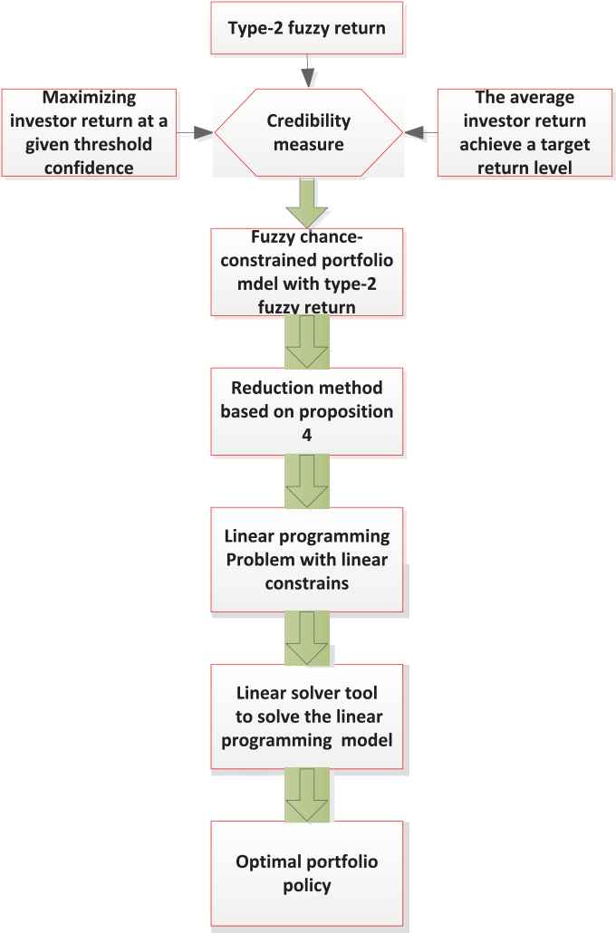
Framework of the method.
5.1. Chance-Constrained Programing Using Generalized Credibility
We formulate a chance-constrained programing model with reduced fuzzy parameters to solve the above problem. By using credibility measures, Liu and Iwamura [72], Yang and Liu [73], and Kundu et al. [74] developed chance-constrained programing with fuzzy parameters. However, the usual credibility measure could not be further used because of the unnormalization of the reduced fuzzy parameters. Thus, using generalized credibility, the problem becomes a maximization problem and can be formulated as the following chance-constrained programing model (36):
Regarding notation, the following generalized credibility is replaced by the usual credibility measure.
5.2. Crisp Equivalence
Proposition 4.
Let ξi be the reduction of the type-2 triangular fuzzy variable
If 0 < α ≤ 0.25, then the equivalent parametric programing problem for the model (36) is
If 0.25 < α ≤ 0.5, then the equivalent parametric programing problem for model (36) is
If 0.5 < α ≤ 0.75, then the equivalent parametric programing problem for model (36) is
If 0.75 < α ≤ 1, then the equivalent parametric programing problem for model (36) is
Proof.
The model formulations for the four cases can be obtained immediately from Propositions 1 and 2.
Proposition 4 may be used to show that the portfolio selection model with type-2 fuzzy return variables is transformed into a linear programing model by the reduction method. There are four cases to be considered per confidence level α (in fact, there are also four cases per confidence curve level β). Theoretically, 16 cases must be considered with respect to four different interval values for both α and β. For each α, there are four cases for different values of β, as can be seen from Eq. (33).
To further elaborate on our main idea, the first step is to reformulate a new type-2 fuzzy portfolio selection model based on a credibility measure; then, using Proposition 4, our proposed model is transformed into an easy linear programing model. We use the six-step algorithm shown in Table 3 to obtain optimal portfolio strategies.
| For Our Type-2 Fuzzy Portfolio Model |
|---|
| Step 1. Input parameters of type-2 fuzzy n assets return, |
| Step 2. Determine the given parameters |
| Step 3. Determine one of four cases in Proposition 4 and formulate a linear programing portfolio model. |
| Step 4. Use a linear programing tool (MATLAB or LINGO) to solve the proposed model. |
| Step 5. Repeat steps 3 and 4. |
| Step 6. Output the optimal portfolio policy |
Algorithm steps for our proposed model.
The portfolio problem is easily solved for these four cases using a linear optimization solver. The next section gives an illustrative example.
6. NUMERICAL EXAMPLE
In this section, we first present an example to show the effectiveness of the proposed model, then we provide a sensitivity analysis for some parameters.
6.1. Performance of the Proposed Model
To illustrate the portfolio choice model (44) and to demonstrate its performance, we provide some illustrative examples. For this purpose, all code is run in MATLAB R2017a. Fuzzy data with respect to type-2 fuzzy return for 20 different assets are provided in the following example. Assume that an investor intends to invest his fund in 20 securities in the market. Let xi be the investment proportion of the securities i, and assume that ξi are the mutually independent type-2 triangular fuzzy returns for i = 1, 2,…, 20. The parametric distributions of,
| ξ1 | r11 | r12 | r13 | θ1,l | θ1,r |
|---|---|---|---|---|---|
| Asset 1 | 0.9946 | 1.0012 | 1.0016 | 0.2058 | 0.8147 |
| ξ2 | r21 | r22 | r23 | θ2,l | θ2,r |
| Asset 2 | 1.0011 | 1.0061 | 1.0092 | 0.3134 | 0.1275 |
| ξ3 | r31 | r32 | r33 | θ3,l | θ3,r |
| Asset 3 | 0.9986 | 1.0081 | 1.0094 | 0.0975 | 0.6324 |
| ξ4 | r41 | r42 | r43 | θ4,l | θ4,r |
| Asset 4 | 0.9983 | 1.0122 | 1.0263 | 0.3469 | 0.2785 |
| ξ5 | r51 | r52 | r53 | θ5,l | θ5,r |
| Asset 5 | 1.0033 | 1.0262 | 1.0310 | 0.2649 | 0.9575 |
| ξ6 | r61 | r62 | r63 | θ6,l | θ6,r |
| Asset 6 | 1.0146 | 1.0248 | 1.0499 | 0.3706 | 0.1576 |
| ξ7 | r71 | r72 | r73 | θ7,l | θ7,r |
| Asset 7 | 1.0209 | 1.0146 | 1.0553 | 0.0854 | 0.9572 |
| ξ8 | r81 | r82 | r83 | θ8,l | θ8,r |
| Asset 8 | 1.0291 | 1.0468 | 1.0679 | 0.1419 | 0.8003 |
| ξ9 | r91 | r92 | r93 | θ9,l | θ9,r |
| Asset 9 | 1.0259 | 1.0818 | 1.0709 | 0.3157 | 0.8218 |
| ξ10 | r101 | r102 | r103 | θ10,l | θ10,r |
| Asset 10 | 1.0350 | 1.0671 | 1.0830 | 0.2595 | 0.7922 |
| ξ11 | r111 | r112 | r113 | θ11,l | θ11,r |
| Asset 11 | 1.0388 | 1.0702 | 1.0851 | 0.0357 | 0.6557 |
| ξ12 | r121 | r122 | r123 | θ12,l | θ12,r |
| Asset 12 | 1.0385 | 1.0758 | 1.0986 | 0.2340 | 0.8491 |
| ξ13 | r131 | r132 | r133 | θ13,l | θ13,r |
| Asset 13 | 1.0414 | 1.0770 | 1.1024 | 0.3577 | 0.6787 |
| ξ14 | r141 | r142 | r143 | θ14,l | θ14,r |
| Asset 14 | 1.0511 | 1.0790 | 1.1116 | 0.1922 | 0.7431 |
| ξ15 | r151 | r152 | r153 | θ15,l | θ15,r |
| Asset 15 | 1.0422 | 1.0877 | 1.1168 | 0.1712 | 0.6555 |
| ξ16 | r161 | r162 | r163 | θ16,l | θ16,r |
| Asset 16 | 1.0373 | 1.0972 | 1.1171 | 0.0318 | 0.7060 |
| ξ17 | r171 | r172 | r173 | θ17,l | θ17,r |
| Asset 17 | 1.0460 | 1.1048 | 1.1269 | 0.0462 | 0.2769 |
| ξ18 | r181 | r182 | r183 | θ18,l | θ18,r |
| Asset 18 | 1.0640 | 1.1130 | 1.1300 | 0.2235 | 0.1971 |
| ξ19 | r191 | r192 | r193 | θ19,l | θ19,r |
| Asset 19 | 1.0615 | 1.1155 | 1.1275 | 0.3171 | 0.6948 |
| ξ20 | r201 | r202 | r203 | θ20,l | θ20,r |
| Asset 20 | 1.0456 | 1.1221 | 1.1257 | 0.0344 | 0.9502 |
Parameters of mutually independent type-2 triangular fuzzy returns for 20 assets.
For simplicity, on the one hand, we first fix the parameters β = 0.2, d = 0.01 and solve the portfolio choice problem; the distributions of the 20 assets are presented in Table 4 for α = 0.2, 0.4, 0.6, 0.8. Given the above parameter settings, we present the allocated money and the results of the model in Table 5, showing that concentrative investment occurs for assets 18 and 5. Actually, in this case, the percentages invested in assets 18 and 5 are around 0.75 ( highly recommended) with respect to parameter α = 0.2, 0.4, 0.6, 0.8.
| α = 0.2 | β = 0.2 | d = 0.01 | |||||||
|---|---|---|---|---|---|---|---|---|---|
| 1 | 2 | 3 | 4 | 5 | 6 | 7 | 8 | 9 | 10 |
| 0.0133 | 0.0133 | 0.0161 | 0.0132 | 0.0130 | 0.0130 | 0.0128 | 0.0127 | 0.0125 | 0.0125 |
| 11 | 12 | 13 | 14 | 15 | 16 | 17 | 18 | 19 | 20 |
| 0.0125 | 0.0124 | 0.0124 | 0.0123 | 0.0123 | 0.0122 | 0.0121 | 0.7572 | 0.0120 | 0.0120 |
| α = 0.4 | β = 0.2 | d = 0.01 | |||||||
| 1 | 2 | 3 | 4 | 5 | 6 | 7 | 8 | 9 | 10 |
| 0.0133 | 0.0133 | 0.0161 | 0.0132 | 0.7585 | 0.0130 | 0.0128 | 0.0127 | 0.0125 | 0.0125 |
| 11 | 12 | 13 | 14 | 15 | 16 | 17 | 18 | 19 | 20 |
| 0.0125 | 0.0124 | 0.0124 | 0.0123 | 0.0123 | 0.0122 | 0.0121 | 0.0120 | 0.0120 | 0.0120 |
| α = 0.6 | β = 0.2 | d = 0.01 | |||||||
| 1 | 2 | 3 | 4 | 5 | 6 | 7 | 8 | 9 | 10 |
| 0.0133 | 0.0133 | 0.0161 | 0.0132 | 0.7582 | 0.0130 | 0.0128 | 0.0127 | 0.0125 | 0.0125 |
| 11 | 12 | 13 | 14 | 15 | 16 | 17 | 18 | 19 | 20 |
| 0.0125 | 0.0124 | 0.0124 | 0.0123 | 0.0123 | 0.0122 | 0.0121 | 0.0120 | 0.0120 | 0.0120 |
| α = 0.8 | β = 0.2 | d = 0.01 | |||||||
| 1 | 2 | 3 | 4 | 5 | 6 | 7 | 8 | 9 | 10 |
| 0.0133 | 0.0133 | 0.0161 | 0.0132 | 0.0130 | 0.0130 | 0.0128 | 0.0127 | 0.0125 | 0.0125 |
| 11 | 12 | 13 | 14 | 15 | 16 | 17 | 18 | 19 | 20 |
| 0.0125 | 0.0124 | 0.0124 | 0.0123 | 0.0123 | 0.0122 | 0.0121 | 0.7572 | 0.0120 | 0.0120 |
Optimal asset allocation given fixed parameters β = 0.2 and d = 0.01.
On the other hand, we fix the parameters, α = 0.2, β = 0.2, taking values d = 0.02 and 0.03. We use the main attributes shown in Table 6 to solve the portfolio choice model. These results show that the allocated money is concentrated on asset 18, which reaches 0.5154 (medium recommended) and 0.2717 (low recommended), respectively. In other words, it is desirable to invest in asset 18, which dominates the portfolio selection compared with the other assets. It can benefit a lot from the combinations in the portfolio. From the results shown in Tables 5 and 6, we can conclude that the relationships between parameter settings and recommended asset levels are as shown in Table 7. In addition, to illustrate the relationship between optimal objective values and various parameters, Table 8 presents the optimal objective values for various fixed parameters. As shown in Table 8, the maximum values of the objective functions depend on the combination of different parameters. Note that in the case where α = 0.8, β = 0.2, d = 0.01, the maximum value of the objective functions is 4.7029, which is greater than that obtained by combining the other parameters.
| α = 0.2 | β = 0.2 | d = 0.01 | |||||||
|---|---|---|---|---|---|---|---|---|---|
| 1 | 2 | 3 | 4 | 5 | 6 | 7 | 8 | 9 | 10 |
| 0.0267 | 0.0265 | 0.0321 | 0.0263 | 0.0261 | 0.0260 | 0.0256 | 0.0255 | 0.0249 | 0.0251 |
| 11 | 12 | 13 | 14 | 15 | 16 | 17 | 18 | 19 | 20 |
| 0.0250 | 0.0248 | 0.0248 | 0.0247 | 0.0246 | 0.0245 | 0.0243 | 0.5154 | 0.0249 | 0.0251 |
| α = 0.2 | β = 0.2 | d = 0.03 | |||||||
| 1 | 2 | 3 | 4 | 5 | 6 | 7 | 8 | 9 | 10 |
| 0.0400 | 0.0398 | 0.0482 | 0.0395 | 0.0391 | 0.0389 | 0.0385 | 0.0382 | 0.0374 | 0.0376 |
| 11 | 12 | 13 | 14 | 15 | 16 | 17 | 18 | 19 | 20 |
| 0.0375 | 0.0373 | 0.0372 | 0.0370 | 0.0369 | 0.0367 | 0.0364 | 0.2717 | 0.0361 | 0.0361 |
Optimal asset allocation given fixed parameters β = 0.2 and α = 0.2.
| Parameter Settings | High | Medium | Low |
|---|---|---|---|
| α = 0.2, β = 0.2, d = 0.01 | Asset 18 | ||
| α = 0.4, β = 0.2, d = 0.01 | Asset 5 | ||
| α = 0.6, β = 0.2, d = 0.01 | Asset 5 | ||
| α = 0.8, β = 0.2, d = 0.01 | Asset 18 | ||
| α = 0.2, β = 0.2, d = 0.02 | Asset 18 | ||
| α = 0.2, β = 0.2, d = 0.03 | Asset 18 |
Recommended asset levels for given parameter settings.
| α | β | d | Optimal Objective Value |
|---|---|---|---|
| 0.2 | 0.2 | 0.01 | 1.0936 |
| 0.4 | 0.2 | 0.01 | 2.6045 |
| 0.6 | 0.2 | 0.01 | 2.5855 |
| 0.8 | 0.2 | 0.01 | 4.7029 |
| 0.2 | 0.2 | 0.02 | 1.0580 |
| 0.2 | 0.2 | 0.03 | 1.0024 |
| 0.6 | 0.4 | 0.02 | 2.3868 |
| 0.6 | 0.8 | 0.02 | 0.9276 |
| 0.6 | 0.6 | 0.02 | 1.0405 |
| 0.8 | 0.6 | 0.03 | 1.0193 |
Optimal objective values for different fixed parameters.
Given this scenario, recall that we desire to invest in 20 assets, so the optimal portfolio must be a combination of these 20 assets and depends on parameters including the investor’s confidence curve, the confidence level, and the maximum risk level that the investor can tolerate. As a numerical example, the risk curve of the optimal money allocation for the portfolio selection is generated, using the parameters listed in Table 8. The whole of the generated portfolio risk curve lies below the investor’s confidence curve. That is, it is safe to invest with this combination of these 20 assets, which reflects the specific investor’s preferences.
6.2. Sensitivity Analysis
In this subsection, we focus on the sensitivity of the model with respect to some important parameters. First, we perform a sensitivity analysis for parameters d and α. The sensitivity results are shown in Figures 2 and 3 for the two parameters, respectively. Figure 2 also shows that the impact on the objective value is reflected in the shape of the normal distribution. Thus, after reaching an objective threshold value, the portfolio selection problem becomes insensitive as the given confidence level of the portfolio moves to a high (i.e., undesirable) level. Figure 3 shows clearly that as increases, the objective value of the generated portfolio decreases. The higher the objective value that the investor tolerates, the lower the return that the investor gains.
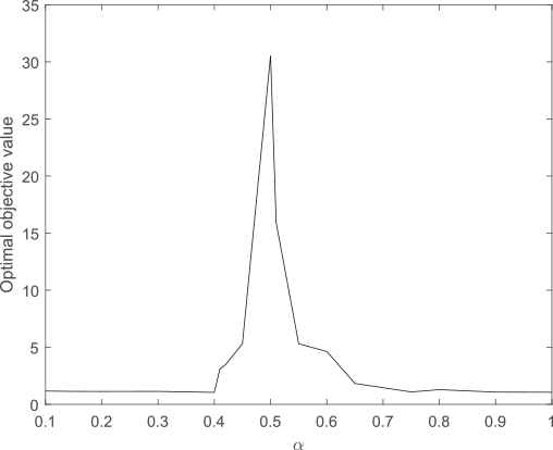
Sensitivity analysis for confidence level.
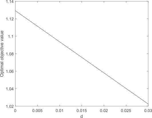
Sensitivity analysis for risk tolerance level.
Next, in line with the setting of [30], we consider a portfolio choice problem with the below confidence curve expression:
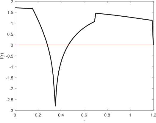
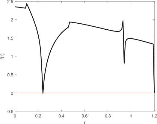
In the following section, we focus on the relationship between the constraints and the optimal solution at different tolerance levels (low, medium, and high). Recall the model constraints that involve β(r); we first define the function f(r) as follows:
We perform a sensitivity analysis with respect to the parameter r on the risk curve. To illustrate the relationship between the optimal solution and the constraints, we first fix the parameters α = 0.2 and d = 0.01. The optimal solutions β(r) for low, medium, and high constraint tolerance are shown in Figures 4–6, respectively. In the low-tolerance case, Figure 4 shows clearly that as increases, f(r) has a V shape. The region below the red line is infeasible. After reaching a value of zero, f(r becomes infeasible as the generated portfolio risk curve moves above the confidence curve of the investor and then enters the undesirable high-risk region. As mentioned earlier, the portfolio fuzzy chance constraints involving β(r [see Eq. (44)] of the model are replaced by the function f(r.
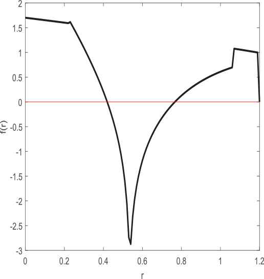
Sensitivity analysis for β(r) for parameters given in Table 9.
| Case I | α = 0.2 | K = 1.3 | d = 0.01 | r = [1.0664, 1.2000] |
| Case II | α = 0.2 | K = 1.3 | d = 0.01 | r = [0.5332, 1.0664] |
| Case III | α = 0.2 | K = 1.3 | d = 0.01 | r = [0.2213, 0.5332] |
| Case IV | α = 0.2 | K = 1.3 | d = 0.01 | r = [0.0000, 0.2213] |
Parameter settings for four cases when K = 1.3.
Sensitivity analysis for parameters given in Table 10.
| Case I | α = 0.2 | K = 2 | d = 0.01 | r = [0.6931, 1.2000] |
| Case II | α = 0.2 | K = 2 | d = 0.01 | r = [0.3466, 0.6931] |
| Case III | α = 0.2 | K = 2 | d = 0.01 | r = [0.1438, 0.3466] |
| Case IV | α = 0.2 | K = 2 | d = 0.01 | r = [0.0000, 0.1438] |
Parameter settings for four cases when K = 2.
Sensitivity analysis for parameters given in Table 11.
| Case I | α = 0.2 | K = 3 | d = 0.01 | r = [0.4621, 1.2000] |
| Case II | α = 0.2 | K = 3 | d = 0.01 | r = [0.2310, 0.4621] |
| Case III | α = 0.2 | K = 3 | d = 0.01 | r = [0.0959, 0.2310] |
| Case IV | α = 0.2 | K = 3 | d = 0.01 | r = [0.0000, 0.0959] |
Parameter settings for four cases when K = 3.
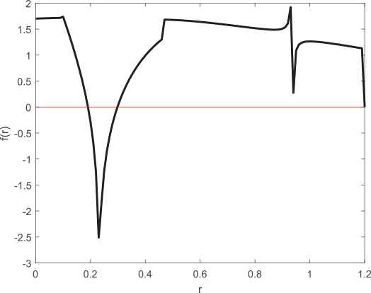
Similar to Figure 4, Figures 5 and 6 illustrate the relationship between f(r) and the severity of the loss for the medium and low tolerance levels, respectively. Figure 5 shows that as increases, the function enters the infeasible region earlier compared with that in Figure 4. After reaching the threshold value, f(r) becomes increasingly “dramatic” and tends to enter feasible regions. However, when it hits the boundary, it goes to zero immediately. As shown in Figure 6, f(r) fluctuates several times after reaching the threshold value, and its terminal value tends to zero. The same phenomenon is observed as in the previous cases, showing that it becomes infeasible as the generated portfolio risk curve moves above the confidence curve of the investor and then enters the undesirable high-risk region. The underlying reason for this is that the violation of such fuzzy chance constraints causes the infeasibility problem.
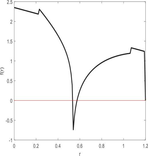
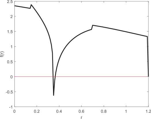
For the three different tolerance levels, we reconsider the relationship f(r) when the parameters, α = 0.6, d = 0.03 are fixed. The severity levels of the loss are shown in Figures 7–9, respectively, and the corresponding parameters are shown in Tables 12–14. The most obvious difference due to the parameter settings is that the infeasible regions become smaller than in the cases shown in Figures 4–6. The numerical results show that the relationship between investor tolerance of portfolio risk and the values attained for the four objective functions is consistent with expectations for the risk–return trade-off.
Sensitivity analysis for β(r) for parameters shown in Table 12.
| Case I | α = 0.6 | K = 1.3 | d = 0.03 | r = [1.0664, 1.2000] |
| Case II | α = 0.6 | K = 1.3 | d = 0.03 | r = [0.5332, 1.0664] |
| Case III | α = 0.6 | K = 1.3 | d = 0.03 | r = [0.2213, 0.5332] |
| Case IV | α = 0.6 | K = 1.3 | d = 0.03 | r = [0.0000, 0.2213] |
Parameter settings for four cases when K = 1.3.
Sensitivity analysis for parameters shown in Table 13.
| Case I | α = 0.6 | K = 2 | d = 0.03 | r = [0.6931, 1.2000] |
| Case II | α = 0.6 | K = 2 | d = 0.03 | r = [0.3466, 0.6931] |
| Case III | α = 0.6 | K = 2 | d = 0.03 | r = [0.1438, 0.3466] |
| Case IV | α = 0.6 | K = 2 | d = 0.03 | r = [0.0000, 0.1438] |
Parameter settings for four cases when K = 2.
Sensitivity analysis for parameters shown in Table 14.
| Case I | α = 0.6 | K = 3 | d = 0.03 | r = [0.4621, 1.2000] |
| Case II | α = 0.6 | K = 3 | d = 0.03 | r = [0.2310, 0.4621] |
| Case III | α = 0.6 | K = 3 | d = 0.03 | r = [0.0959, 0.2310] |
| Case IV | α = 0.6 | K = 3 | d = 0.03 | r = [0.0000, 0.0959] |
Parameter settings for four cases when K = 3.
6.3. Comparison of Performance with Other Methods
In this subsection, AHP, TOPSIS, HIA, and GA are selected as benchmark methods with which to compare the performance of our proposed method. In particular, we calculate the CPU running time as a performance index. The test results are shown in Table 15. Owing to the insensitivity of running CPU time for the above-mentioned four cases, we only calculate it for Case I, setting the following parameters, α = 0.2, K = 1.3, d = 0.01, r = [1.0664, 1.2000]. As the number of assets increases, we use MATLAB to generate randomly type-2 triangular fuzzy returns with preset fixed right and left parameters (see Table 4). The results shown in Table 15 indicate that our proposed reduction method has superior performance compared with other methods.
| Method | AHP | TOPSIS | HIA | GA | Our Method |
|---|---|---|---|---|---|
| Number of Assets | Time | Time | Time | Time | Time |
| n = 20 | 0.10 s | 0.11 s | 0.10 s | 0.10 s | 0.10 s |
| n = 50 | 0.20 s | 0.23 s | 0.28 s | 0.11 s | 0.10s |
| n = 100 | 0.25 s | 0.35 s | 0.30 s | 0.25 s | 0.10 s |
| n = 1000 | 0.50 s | 0.49 s | 27 s | 25 s | 0.20 s |
| n = 10000 | 1.50 s | 1.60 s | 50 s | >1 min | 0.25 s |
Performance comparisons with other methods.
7. CONCLUSION
In this paper, we reformulate type-2 fuzzy returns of the portfolio selection problem using chance-constrained programing. The uncertain variables used here focus on the portfolio return for type-2 fuzzy variables. We use an analytical reduction method to transform type-2 fuzzy variables into type-1 fuzzy variables, and the chance-constrained programing model based on a credibility measure is transformed into a linear programing model. Furthermore, we present a numerical example involving different confidence curves for portfolio selection. The numerical results show that the relationship between investor tolerance of portfolio risk and values attained by the objective functions is consistent with the risk–return trade-off. We also performed numerical experiments to reflect investor preferences with respect to the objective functions; the results are shown to be nearly linear with investor special preferences. The comparisons of the results of the numerical analysis clearly show both the efficiency of the reduction method and the good performance of the model in different situations.
Note that the proposed model also has some limitations; in particular, a large number of problems exist that cannot be transformed into linear programing problems. Future possible work includes extending the model by considering the higher-order moment of the risky returns in a type-2 fuzzy environment (i.e., considering skewness as another essential criterion). Another future direction would be to make use of heuristic algorithms to solve more realistic portfolio choice problems associated with type-2 fuzzy variables, such as strategic supplier selection problems, sustainable supplier selection problems, and low carbon supplier selection. Regarding multi-attribute portfolio selection problems, there are other possible methods; for instance, some novel operators, Maclaurin symmetric mean operators, Heronian mean operators, entropy measures, and the TOPSIS method have been applied to solve complex multi-attribute decision-making problems [75–78].
CONFLICTS OF INTEREST
The authors declare they have no conflicts of interest.
AUTHORS' CONTRIBUTIONS
Guang Yang: Methodology, Formal analysis, Funding acquisition, Writing - review & editing. Mei Cai: Validation, Funding acquisition, Writing - review & editing, Xinwang Liu: Validation, Funding acquisition, Writing-review & editing, Supervision. Jindong Qin: Validation, Funding acquisition, Writing-review & editing, Supervision. Xu Zhang: Validation, Funding acquisition, Writing - review & edit.
ACKNOWLEDGMENTS
The authors gratefully acknowledge financial support from the National Science Foundation of China (grant nos. 71871121, 71903097, 72071045, 72071151), the Startup Foundation for Introducing Talent of NUIST (grant no. 1441182001002), the General Project of Philosophy and Social Science Research in Colleges and Universities in Jiangsu Province (grant no. 2020SJA0174), the Natural Science Foundation of Jiangsu Province (BK20190767), the Ministry of Education in China Project of Humanities and Social Sciences (17YJC630114), and the Natural Science Foundation of Hubei Province (2020CFB773). The authors thank the editors and the anonymous reviewers for their valuable comments and suggestions that have greatly improved the quality of this paper.
REFERENCES
Cite this article
TY  - JOUR
AU  - Guang Yang
AU  - Mei Cai
AU  - Jindong Qin
AU  - Xinwang Liu
AU  - Xu Zhang
PY  - 2021
DA  - 2021/05/26
TI  - Analytical Reduction Method for New Type-2 Fuzzy Chance-Constrained Portfolio Selection Model
JO  - International Journal of Computational Intelligence Systems
SP  - 1617
EP  - 1632
VL  - 14
IS  - 1
SN  - 1875-6883
UR  - https://doi.org/10.2991/ijcis.d.210507.001
DO  - 10.2991/ijcis.d.210507.001
ID  - Yang2021
ER  -