International Journal of Computational Intelligence Systems

Volume 14, Issue 1, 2021, Pages 1653 - 1671

Some Cosine Similarity Measures and Distance Measures between Complex q-Rung Orthopair Fuzzy Sets and Their Applications

Authors
Peide Liu1, *, ORCID, Zeeshan Ali2, Tahir Mahmood2, ORCID
1School of Management Science and Engineering, Shandong University of Finance and Economics, Jinan, 250015, China
2Department of Mathematics and Statistics, International Islamic University, Islamabad, 44000, Pakistan
*Corresponding author. Email: peide.liu@gmail.com
Corresponding Author
Peide Liu
Received 21 March 2021, Accepted 25 May 2021, Available Online 10 June 2021.
DOI
10.2991/ijcis.d.210528.002How to use a DOI?
Keywords
Complex q-rung orthopair fuzzy sets; Cosine similarity measures; Cosine distance measures; Technique for an order of preference by similarity to ideal solution
Abstract

As a modification of the q-rung orthopair fuzzy sets (QROFSs), complex QROFSs (CQROFSs) can describe the inaccurate information by complex-valued truth grades with an additional term, named as phase term. Cosine similarity measures (CSMs) and distance measures (DMs) are important tools to verify the grades of discrimination between the two sets. In this manuscript, we develop some CSMs and DMs for CQROFSs. Firstly, the CSMs and Euclidean DMs (EDMs) for CQROFSs and their properties are investigated. Because the CSMs do not keep the axiom of similarity measure (SM), we investigate a technique to develop other SMs based on CQROFSs, and they meet the axiom of the SMs. Moreover, we propose a cosine DM (CDM) based on CQROFSs by considering the interrelationship among the SMs and DMs, then we propose an extended TOPSIS method to solve the multi-attribute decision-making problems. Finally, we provide some sensible examples to demonstrate the practicality and efficiency of the suggested procedure, at the same time, the graphical representations of the developed measures are also utilized in this manuscript.

Copyright
© 2021 The Authors. Published by Atlantis Press B.V.
Open Access
This is an open access article distributed under the CC BY-NC 4.0 license (http://creativecommons.org/licenses/by-nc/4.0/).

1. INTRODUCTION

For a real example, when an institute chooses whether to enroll a tutoring team, a ten-representative committee of authorities evaluated the selected persons, seven of them approved to employ these persons, two of them gave negative opinion, and the additional one did not give any judgment. To characterize this result, an intuitionistic fuzzy set (IFS) was presented by Atanassov [1] to express this kind of information by including a falsity grade based on the fuzzy set (FS) [2] The truth and the falsity in IFS meet a rule that the sum of both of them is restricted to [0, 1]. Now IFS has received extensive attentions from many scholars and has been widely utilized in the different decision areas [3–7]. Due to some complications of decision environment, sometimes, it is difficult for IFS to describe some daily life issues, for instance, if a person gives 0.6 for truth grade and 0.5 for falsity, then the sum of both values is beyond the scope of [0, 1], the IFS is not able to express this type of information accurately. Therefore, Yager [8] proposed the Pythagorean FS (PFS) which is a proficient and capable technique to express complex information for the decision-making problems. The truth and falsity in PFS meet a rule that the sum of the squares of them is in [0, 1]. The PFS has been widely utilized in the different decision making areas [9–14]. Similarly, if a person gives 0.9 for truth grade and 0.8 for falsity, then the sum of the squares of both values is not in [0, 1], the PFS is not able to express this type of information accurately. Therefore, Yager [15] proposed the q-rung orthopair FS (QROFS) to solve this issue. The truth and falsity in QROFS meet a rule that the sum of the q-powers of them is restricted to [0, 1]. Now the QROFS has received extensive attentions from many scholars and has been widely utilized in the different areas [16–19].

To process complex fuzzy information, the truth and falsity degrees are modified from a real subset to the unit disc of the complex plane, and then Alkouri and Salleh [20] established the complex IFS (CIFS) by including the complex-valued falsity on the basis of complex FS (CFS) [21] to handle complex information. The truth and falsity in CIFS meet the rule that the sum of the real parts (also for imaginary parts) of them is restricted to [0, 1]. The CIFS has received extensive attentions from many scholars and has been widely utilized in the different areas [22–25]. However, the CIFS is not able to process some problems, for instance, if a person gives 0.6ei2π7 for truth grade and 0.5ei2π6 for falsity, then the sum of the real parts (also for imaginary parts) of both values is beyond the scope of [0, 1]. Therefore, Ullah et al. [26] proposed the complex PFS (CPFS) in which the truth and falsity meet the rule that the sum of the squares of the real parts (also for imaginary parts) of them is restricted to [0, 1]. The CPFS has received extensive attentions from scholars and has been widely utilized in the different areas [27]. Similarly, if a person gives 0.9ei2π8 for truth grade and 0.8ei2π7 for falsity, then the sum of the squares of the real parts (also for imaginary parts) of them is beyond the scope of [0, 1], the CPFS is not able to describe this type of information accurately. Therefore, Liu et al. [28,29] proposed the complex QROFS (CQROFS) in which the truth and falsity meet the rule that the sum of the q-powers of the real parts (also for imaginary parts) of them is restricted to [0, 1]. The CQROFS has received extensive attentions from many scholars and has been widely utilized in the different areas [30–36].

In real decision problems, we go over numerous circumstances where we need to measure the vulnerability existing in the information to get one ideal choice. Data measures are significant tools for taking care of uncertain information presented in our day-to-day life issues. Different measures of information, such as similarity, distance, entropy, and inclusion, can process the uncertain information and facilitate us to reach some conclusions. Recently, these measures have gained much attention from many scholars due to their wide applications in various fields, such as pattern recognition, medical diagnosis, clustering analysis, and image segment. All the prevailing approaches of decision-making, based on information measures for PFS and QROFS, can only deal with the real-valued truth and falsity grades. In CQROFS, truth and falsity grades are complex-values and are represented in polar coordinates. The amplitudes corresponding to truth and falsity degrees give the extents of membership and nonmembership of an object in a CQROFS with a rule that the sum of the q-powers of the real and unreal parts of both grades is restricted to the unit interval. The phase parts are novel parameters of the truth and falsity degrees added from traditional QROFS. QROFS can deal with only one dimension at a time, which results in information loss in some instances. However, in real life, we come across complex natural phenomena where only one dimensional information cannot express fully the evaluation value, and the second dimensional information is needed to express the truth and falsity grades. By adding the second dimension, the complete information can be projected in one set, and hence, loss of information can be avoided. To illustrate the significance of the phase term, we give an example. Assume XYZ organization chooses to set up biometric-based participation gadgets (BBPGs) in the entirety of its workplaces spread everywhere in the country. For this, the organization counsels a specialist who gives the data concerning (i) demonstrates of BBPGs and (ii) creation dates of BBPGs. The organization needs to choose the most ideal model of BBPGs with its creation date all the while. Here, this issue is two-dimensional, to be specific, the model of BBPGs and the creation date of BBPGs. This kind of issue cannot be expressed precisely by the conventional QROFS. The most ideal approach to address this problem is by utilizing the CQROFS. The amplitudes in CQROFS might be utilized to give the organization's choice regarding the model of BBPGs and the phase parts might be utilized to address the organization's judgment concerning the creation date of BBPGs.

In addition, cosine similarity is one of the most important measures, which can not only compare one data entity with others but also show the extents of association between them and their direction. Also, CQROFSs have a powerful ability to model the imprecise and ambiguous information in real-world applications than the existing information expressions such as CFSs, CIFSs, CPFSs. Besides, the SM is a valid tool to examine the interrelationships among any number of CQROFSs, and it has been utilized to different areas [34]. Rani and Garg [23] investigated the distance similarity by using CIFS. Garg and Rani [37] proposed some information measures based on CIFS. Garg and Rani [24] developed the robust correlation coefficient based on CIFS. But up to date, the SMs for CQROFSs have not been investigated. Because the CQROFSs are a reliable technique to express complex fuzzy information, and the SM is an important tool for decision-making problems, it is necessary to develop some SMs for CQROFSs. Therefore, keeping the advantages of SMs and CQROFSs, the main investigations of this manuscript are summarized as follows:

  1. The cosine similarity measures (CSMs) and Euclidean distance measures (EDMs) for CQROFSs and their properties are investigated.

  2. Considering that the CSMs do not meet the axiom of similarity measure (SM), some new SMs based on CQROFSs using the explored CSMs and EDMs are developed, which meets the axiom of the SMs.

  3. Cosine DMs (CDMs) based on CQROFSs by considering the interrelationship among the SM and DMs are proposed and an extended TOPSIS method is developed.

  4. Some examples are given to demonstrate the practicality and efficiency of the suggested procedure.

  5. The graphical representations of the developed measures are also given in this manuscript.

This manuscript is summarized as follows: In Section 2, we briefly recall the concept of CIFSs, CPFSs, CQROFSs, and their fundamental laws. In Section 3, we develop the CSMs and DMs by using CQROFNs. In Section 4, we develop the TOPSIS method based on the investigated measures. In Section 5, we give a comparative analysis of the proposed work with some existing approaches. The conclusion of this manuscript is discussed in Section 6.

2. PRELIMINARIES

In this work, we recall the main ideas of CIFSs, CPFSs, CQROFSs, and their fundamental laws. We use the symbol O⏞ for universal sets and the truth and falsity degrees are shown by MℭCQ and NℭCQ, where MℭCQo⏞=MℭRPo⏞ei2πMℭIPo⏞ and NℭCQo⏞=NℭRPo⏞ei2πNℭIPo⏞.

Definition 1.

[20] A CIFS ℭCQ is demonstrated by

ℭCQ=MℭCQo⏞,NℭCQo⏞:o⏞∈O⏞(1)
where MℭCQo⏞=MℭRPo⏞ei2πMℭIPo⏞ and NℭCQo⏞=NℭRPo⏞ei2πNℭIPo⏞ express the truth degree and the falsity degree with 0≤MℭRPo⏞+NℭRPo⏞≤1 and 0≤MℭIPo⏞+NℭIPo⏞≤1. Moreover, the term ℐℭCQo⏞=ℐℭRPo⏞ei2πℐℭIP=1−MℭRPo⏞−NℭRPo⏞ei2π1−MℭIPo⏞−NℭIPo⏞ expresses the degree of indeterminacy.

Definition 2.

[26] A CPFS ℭCQ is demonstrated by

ℭCQ=MℭCQo⏞,NℭCQo⏞:o⏞∈O⏞(2)
where MℭCQo⏞=MℭRPo⏞ei2πMℭIPo⏞ and NℭCQo⏞=NℭRPo⏞ei2πNℭIPo⏞ express the truth degree and the falsity degree with 0≤MℭRP2o⏞+NℭRP2o⏞≤1 and 0≤MℭIP2o⏞+NℭIP2o⏞≤1. Moreover, the term ℐℭCQo⏞=ℐℭRPo⏞ei2πℐℭIP=1−MℭRP2o⏞−NℭRP2o⏞12ei2π1−MℭIP2o⏞−NℭIP2o⏞12 expresses the degree of indeterminacy.

Definition 3.

[28,29] A CQROFS ℭCQ is demonstrated by

ℭCQ=MℭCQo⏞,NℭCQo⏞:o⏞∈O⏞(3)
where MℭCQo⏞=MℭRPo⏞ei2πMℭIPo⏞ and NℭCQo⏞=NℭRPo⏞ei2πNℭIPo⏞ express the truth degree and the falsity degree with 0≤MℭRPqCQo⏞+NℭRPqCQo⏞≤1 and 0≤MℭIPqCQo⏞+NℭIPqCQo⏞≤1,qCQ≥1. Moreover, the term ℐℭCQo⏞=ℐℭRPo⏞ei2πℐℭIP=1−MℭRPqCQo⏞−NℭRPqCQo⏞1qCQei2π1−MℭIPqCQo⏞−NℭIPqCQo⏞1qCQ expresses the degree of indeterminacy. Throughout, this manuscript, the complex q-rung orthopair fuzzy numbers (CQROFNs) are shown by ℭCQ=MℭRPei2πMℭIP,NℭRPei2πNℭIP. Further, we define the score and accuracy values such that
SCQℭCQ=12MℭRPqCQ+MℭIPqCQ−NℭRPqCQ−NℭIPqCQ,SCQℭCQ∈−1,1(4)
ℌCQℭCQ=12MℭRPqCQ+MℭIPqCQ+NℭRPqCQ+NℭIPqCQ,ℌCQℭCQ∈0,1(5)

To find the relationships between any two CQROFNs ℭCQ−1=MℭRP−1ei2πMℭIP−1,NℭRP−1ei2πNℭIP−1 and ℭCQ−2=MℭRP−2ei2πMℭIP−2,NℭRP−2ei2πNℭIP−2, we use the following rules:

  1. If SCQℭCQ−1>SCQℭCQ−2⇒ℭCQ−1>ℭCQ−2;

  2. If SCQℭCQ−1<SCQℭCQ−2⇒ℭCQ−1<ℭCQ−2;

  3. If SCQℭCQ−1=SCQℭCQ−2⇒;

    1. If ℌCQℭCQ−1>ℌCQℭCQ−2⇒ℭCQ−1>ℭCQ−2;

    2. If ℌCQℭCQ−1<ℌCQℭCQ−2⇒ℭCQ−1<ℭCQ−2.

3. CSMs AND DMs BETWEEN CQROFSs

In this part, some CSMs and DMs for CQROFSs are proposed.

Definition 4.

For any two CQROFNs ℭCQ−1=MℭRP−1oi⏞ei2πMℭIP−1oi⏞,NℭRP−1oi⏞ei2πNℭIP−1oi⏞ and ℭCQ−2=MℭRP−2oi⏞ei2πMℭIP−2oi⏞,NℭRP−2oi⏞ei2πNℭIP−2oi⏞,i=1,2,,...,n˜, based on a universal set O⏞=o1⏞,o2⏞,…,on˜⏞, then the CSM CSMCQℭCQ−1,ℭCQ−2 is demonstrated by

CSMCQℭCQ−1,ℭCQ−2=1n˜∑i=1n˜MℭRP−1qCQoi⏞MℭRP−2qCQoi⏞+MℭIP−1qCQoi⏞MℭIP−2qCQoi⏞+NℭRP−1qCQoi⏞NℭRP−2qCQoi⏞+NℭIP−1qCQoi⏞NℭIP−2qCQoi⏞MℭRP−12qCQoi⏞+MℭIP−12qCQoi⏞+NℭRP−12qCQoi⏞+NℭIP−12qCQoi⏞×MℭRP−22qCQoi⏞+MℭIP−22qCQoi⏞+NℭRP−22qCQoi⏞+NℭIP−22qCQoi⏞(6)

Theorem 1.

For any two CQROFNs ℭCQ−1=MℭRP−1oi⏞ei2πMℭIP−1oi⏞,NℭRP−1oi⏞ei2πNℭIP−1oi⏞ and ℭCQ−2=MℭRP−2oi⏞ei2πMℭIP−2oi⏞,NℭRP−2oi⏞ei2πNℭIP−2oi⏞,i=1,2,,...,n˜, based on a universal set O⏞=o1⏞,o2⏞,…,on˜⏞, then the CSM CSMCQℭCQ−1,ℭCQ−2 holds the following conditions:

  1. 0≤CSMCQℭCQ−1,ℭCQ−2≤1;

  2. CSMCQℭCQ−1,ℭCQ−2=CSMCQℭCQ−2,ℭCQ−1;

  3. CSMCQℭCQ−1,ℭCQ−2=1 if ℭCQ−1=ℭCQ−2 that is MℭRP−1=MℭRP−2,MℭIP−1=MℭIP−2NℭRP−1=NℭRP−2,NℭIP−1=NℭIP−2.

Proof:

Based on Definition 4, conditions (1) and (2) are straightforward. Moreover, if we choose the ℭCQ−1=ℭCQ−2, that is, MℭRP−1=MℭRP−2,MℭIP−1=MℭIP−2NℭRP−1=NℭRP−2,NℭIP−1=NℭIP−2, then

CSMCQℭCQ−1,ℭCQ−2=1n˜∑i=1n˜MℭRP−1qCQoi⏞MℭRP−2qCQoi⏞+MℭIP−1qCQoi⏞MℭIP−2qCQoi⏞+NℭRP−1qCQoi⏞NℭRP−2qCQoi⏞+NℭIP−1qCQoi⏞NℭIP−2qCQoi⏞MℭRP−12qCQoi⏞+MℭIP−12qCQoi⏞+NℭRP−12qCQoi⏞+NℭIP−12qCQoi⏞×MℭRP−22qCQoi⏞+MℭIP−22qCQoi⏞+NℭRP−22qCQoi⏞+NℭIP−22qCQoi⏞=1n˜∑i=1n˜MℭRP−1qCQoi⏞MℭRP−1qCQoi⏞+MℭIP−1qCQoi⏞MℭIP−1qCQoi⏞+NℭRP−1qCQoi⏞NℭRP−1qCQoi⏞+NℭIP−1qCQoi⏞NℭIP−1qCQoi⏞MℭRP−12qCQoi⏞+MℭIP−12qCQoi⏞+NℭRP−12qCQoi⏞+NℭIP−12qCQoi⏞×MℭRP−12qCQoi⏞+MℭIP−12qCQoi⏞+NℭRP−12qCQoi⏞+NℭIP−12qCQoi⏞=1n˜∑i=1n˜MℭRP−12qCQoi⏞+MℭIP−12qCQoi⏞+NℭRP−12qCQoi⏞+NℭIP−12qCQoi⏞MℭRP−12qCQoi⏞+MℭIP−12qCQoi⏞+NℭRP−12qCQoi⏞+NℭIP−12qCQoi⏞12+12=1.

Hence, we obtain CSMCQℭCQ−1,ℭCQ−2=1.

By using the weight vector ΩWV=ΩWV−1,ΩWV−2,…,ΩWV−n˜ with ∑i=1n˜ΩWV−i=1,ΩWV−i∈0,1, then the WCSM is given by

Definition 5.

For any two CQROFNs ℭCQ−1=MℭRP−1oi⏞ei2πMℭIP−1oi⏞,NℭRP−1oi⏞ei2πNℭIP−1oi⏞ and ℭCQ−2=MℭRP−2oi⏞ei2πMℭIP−2oi⏞,NℭRP−2oi⏞ei2πNℭIP−2oi⏞,i=1,2,,...,n˜, based on a universal set O⏞=o1⏞,o2⏞,…,on˜⏞, then the WCSM WCSMCQℭCQ−1,ℭCQ−2 is defined by

WCSMCQℭCQ−1,ℭCQ−2=∑i=1n˜ΩWV−iMℭRP−1qCQoi⏞MℭRP−2qCQoi⏞+MℭIP−1qCQoi⏞MℭIP−2qCQoi⏞+NℭRP−1qCQoi⏞NℭRP−2qCQoi⏞+NℭIP−1qCQoi⏞NℭIP−2qCQoi⏞MℭRP−12qCQoi⏞+MℭIP−12qCQoi⏞+NℭRP−12qCQoi⏞+NℭIP−12qCQoi⏞×MℭRP−22qCQoi⏞+MℭIP−22qCQoi⏞+NℭRP−22qCQoi⏞+NℭIP−22qCQoi⏞(7)

For any two CQROFNs ℭCQ−1=MℭRP−1oi⏞ei2πMℭIP−1oi⏞,NℭRP−1oi⏞ei2πNℭIP−1oi⏞ and ℭCQ−2=MℭRP−2oi⏞ei2πMℭIP−2oi⏞,NℭRP−2oi⏞ei2πNℭIP−2oi⏞,i=1,2,,...,n˜, based on a universal set O⏞, if we choose the weight vector ΩWV=ΩWV−1,ΩWV−2,…,ΩWV−n˜=1n˜,1n˜,…,1n˜, then the WCSMCQℭCQ−1,ℭCQ−2 is reduced to CSMCQℭCQ−1,ℭCQ−2.

Theorem 2.

For any two CQROFNs ℭCQ−1=MℭRP−1oi⏞ei2πMℭIP−1oi⏞,NℭRP−1oi⏞ei2πNℭIP−1oi⏞ and ℭCQ−2=MℭRP−2oi⏞ei2πMℭIP−2oi⏞,NℭRP−2oi⏞ei2πNℭIP−2oi⏞,i=1,2,,...,n˜, based on a universal set O⏞=o1⏞,o2⏞,…,on˜⏞, then the WCSM WCSMCQℭCQ−1,ℭCQ−2 holds the following conditions:

  1. 0≤WCSMCQℭCQ−1,ℭCQ−2≤1;

  2. WCSMCQℭCQ−1,ℭCQ−2=WCSMCQℭCQ−2,ℭCQ−1;

  3. WCSMCQℭCQ−1,ℭCQ−2=1 if ℭCQ−1=ℭCQ−2 that is MℭRP−1=MℭRP−2,MℭIP−1=MℭIP−2NℭRP−1=NℭRP−2,NℭIP−1=NℭIP−2.

Proof:

All are omitted.

Example 1.

Based on the universal set O⏞=o1⏞,o2⏞,o3⏞,o4⏞,o5⏞, two CQROFNs are ℭCQ−1=o1⏞,0.2ei2π0.21,0.5ei2π0.51,o2⏞,0.4ei2π0.41,0.2ei2π0.21,o3⏞,0.5ei2π0.51,0.4ei2π0.41,o4⏞,0.3ei2π0.31,0.3ei2π0.31,o5⏞,0.7ei2π0.71,0.1ei2π0.11 andℭCQ−2=o1⏞,0.2ei2π0.21,0.7ei2π0.71,o2⏞,0.6ei2π0.61,0.3ei2π0.31,o3⏞,0.4ei2π0.41,0.3ei2π0.31,o4⏞,0.4ei2π0.41,0.4ei2π0.41,o5⏞,0.6ei2π0.61,0.1ei2π0.11, further, suppose qCQ=3, and ΩWV=ΩWV−1,ΩWV−2,ΩWV−3,ΩWV−4,ΩWV−5=0.35,0.2,0.1,0.15,0.2, then we can get WCSMCQℭCQ−1,ℭCQ−2=0.99938. If we ignore the imaginary parts in all the above information, then we get WCSMCQℭCQ−1,ℭCQ−2=0.999438, which is discussed in Ref. [38]. When an SM holds the conditions of SMs, then it is called the original SM.

Lemma 1.

For any two FSs ℭCQ−1 and ℭCQ−2, if an SM SMCQℭCQ−1,ℭCQ−2 holds the following axioms:

  1. 0≤SMCQℭCQ−1,ℭCQ−2≤1;

  2. SMCQℭCQ−1,ℭCQ−2=SMCQℭCQ−2,ℭCQ−1;

  3. SMCQℭCQ−1,ℭCQ−2=1 if ℭCQ−1=ℭCQ−2.

Then, we say that the SMCQℭCQ−1,ℭCQ−2 is called the original SM. Where the DM is given by DMCQℭCQ−1,ℭCQ−2=1−SMCQℭCQ−1,ℭCQ−2 based on SM. Moreover, we develop the EDM EDMCQℭCQ−1,ℭCQ−2, which is demonstrated below.

Definition 6.

For any two CQROFNs ℭCQ−1=MℭRP−1oi⏞ei2πMℭIP−1oi⏞,NℭRP−1oi⏞ei2πNℭIP−1oi⏞ and ℭCQ−2=MℭRP−2oi⏞ei2πMℭIP−2oi⏞,NℭRP−2oi⏞ei2πNℭIP−2oi⏞,i=1,2,,...,n˜, based on a universal set O⏞=o1⏞,o2⏞,…,on˜⏞, then the EDM EDMCQℭCQ−1,ℭCQ−2 is defined by

EDMCQℭCQ−1,ℭCQ−2=14n˜∑oi⏞∈O⏞MℭRP−1qCQoi⏞−MℭRP−2qCQoi⏞2+MℭIP−1qCQoi⏞−MℭIP−2qCQoi⏞2+NℭRP−1qCQoi⏞−NℭRP−2qCQoi⏞2+NℭIP−1qCQoi⏞−NℭIP−2qCQoi⏞212(8)

By using the weight vector ΩWV=ΩWV−1,ΩWV−2,…,ΩWV−n˜ meeting ∑i=1n˜ΩWV−i=1,ΩWV−i∈0,1, then the WEDM WEDMCQℭCQ−1,ℭCQ−2 is defined below.

WEDMCQℭCQ−1,ℭCQ−2=14∑oi⏞∈O⏞ΩWV−iMℭRP−1qCQoi⏞−MℭRP−2qCQoi⏞2+MℭIP−1qCQoi⏞−MℭIP−2qCQoi⏞2+NℭRP−1qCQoi⏞−NℭRP−2qCQoi⏞2+NℭIP−1qCQoi⏞−NℭIP−2qCQoi⏞212(9)

Theorem 3.

For any two CQROFNs ℭCQ−1=MℭRP−1oi⏞ei2πMℭIP−1oi⏞,NℭRP−1oi⏞ei2πNℭIP−1oi⏞ and ℭCQ−2=MℭRP−2oi⏞ei2πMℭIP−2oi⏞,NℭRP−2oi⏞ei2πNℭIP−2oi⏞,i=1,2,,...,n˜, based on a universal set O⏞=o1⏞,o2⏞,…,on˜⏞, then the WEDMCQℭCQ−1,ℭCQ−2 holds the following conditions:

  1. 0≤WEDMCQℭCQ−1,ℭCQ−2≤1;

  2. WEDMCQℭCQ−1,ℭCQ−2=WEDMCQℭCQ−2,ℭCQ−1;

  3. WEDMCQℭCQ−1,ℭCQ−2=0 if ℭCQ−1=ℭCQ−2 that is MℭRP−1=MℭRP−2,MℭIP−1=MℭIP−2NℭRP−1=NℭRP−2,NℭIP−1=NℭIP−2.

Proof:

  1. Based on Definition 6, we know that 0≤MℭRP−1,MℭRP−2,MℭIP−1,MℭIP−2NℭRP−1,NℭRP−2,NℭIP−1,NℭIP−2≤1 and the parameter qCQ>0, then 0≤MℭRP−1qCQoi⏞−MℭRP−2qCQoi⏞2≤1,0≤MℭIP−1qCQoi⏞−MℭIP−2qCQoi⏞2≤1,0≤NℭRP−1qCQoi⏞−NℭRP−2qCQoi⏞2≤1 and 0≤NℭIP−1qCQoi⏞−NℭIP−2qCQoi⏞2≤1. Therefore, 0≤WEDMCQℭCQ−1,ℭCQ−2≤14124∑oi⏞∈O⏞ΩWV−i12=1.

  2. By using Definition 6, we easily obtain the WEDMCQℭCQ−1,ℭCQ−2=WEDMCQℭCQ−2,ℭCQ−1.

  3. WEDMCQℭCQ−1,ℭCQ−2=0⇔MℭRP−1qCQoi⏞−MℭRP−2qCQoi⏞2=0, MℭIP−1qCQoi⏞−MℭIP−2qCQoi⏞2=0,NℭRP−1qCQoi⏞−NℭRP−2qCQoi⏞2=0, NℭIP−1qCQoi⏞−NℭIP−2qCQoi⏞2=0 that is MℭRP−1=MℭRP−2,MℭIP−1=MℭIP−2NℭRP−1=NℭRP−2,NℭIP−1=NℭIP−2⇔ℭCQ−1=ℭCQ−2.

Definition 7.

For any two CQROFNs ℭCQ−1=MℭRP−1oi⏞ei2πMℭIP−1oi⏞,NℭRP−1oi⏞ei2πNℭIP−1oi⏞ and ℭCQ−2=MℭRP−2oi⏞ei2πMℭIP−2oi⏞,NℭRP−2oi⏞ei2πNℭIP−2oi⏞,i=1,2,,...,n˜, based on a universal set O⏞=o1⏞,o2⏞,…,on˜⏞, then the new SM NSMCQℭCQ−1,ℭCQ−2 is demonstrated by

NSMCQℭCQ−1,ℭCQ−2=CSMCQℭCQ−1,ℭCQ−2+1−EDMCQℭCQ−1,ℭCQ−22(10)
where
CSMCQℭCQ−1,ℭCQ−2=1n˜∑i=1n˜MℭRP−1qCQoi⏞MℭRP−2qCQoi⏞+MℭIP−1qCQoi⏞MℭIP−2qCQoi⏞+NℭRP−1qCQoi⏞NℭRP−2qCQoi⏞+NℭIP−1qCQoi⏞NℭIP−2qCQoi⏞MℭRP−12qCQoi⏞+MℭIP−12qCQoi⏞+NℭRP−12qCQoi⏞+NℭIP−12qCQoi⏞×MℭRP−22qCQoi⏞+MℭIP−22qCQoi⏞+NℭRP−22qCQoi⏞+NℭIP−22qCQoi⏞
EDMCQℭCQ−1,ℭCQ−2=14n˜∑oi⏞∈O⏞MℭRP−1qCQoi⏞−MℭRP−2qCQoi⏞2+MℭIP−1qCQoi⏞−MℭIP−2qCQoi⏞2+NℭRP−1qCQoi⏞−NℭRP−2qCQoi⏞2+NℭIP−1qCQoi⏞−NℭIP−2qCQoi⏞212

By using the weight vector ΩWV=ΩWV−1,ΩWV−2,…,ΩWV−n˜ meeting ∑i=1n˜ΩWV−i=1,ΩWV−i∈0,1, then the weighted new SM WNSMCQℭCQ−1,ℭCQ−2 is defined as follows.

Definition 8.

For any two CQROFNs ℭCQ−1=MℭRP−1oi⏞ei2πMℭIP−1oi⏞,NℭRP−1oi⏞ei2πNℭIP−1oi⏞ and ℭCQ−2=MℭRP−2oi⏞ei2πMℭIP−2oi⏞,NℭRP−2oi⏞ei2πNℭIP−2oi⏞,i=1,2,,...,n˜, based on a universal set O⏞=o1⏞,o2⏞,…,on˜⏞, then the WNSMCQℭCQ−1,ℭCQ−2 is demonstrated by

NSMCQℭCQ−1,ℭCQ−2=WCSMCQℭCQ−1,ℭCQ−2+1−WEDMCQℭCQ−1,ℭCQ−22(11)
where
WCSMCQℭCQ−1,ℭCQ−2=∑i=1n˜ΩWV−iMℭRP−1qCQoi⏞MℭRP−2qCQoi⏞+MℭIP−1qCQoi⏞MℭIP−2qCQoi⏞+NℭRP−1qCQoi⏞NℭRP−2qCQoi⏞+NℭIP−1qCQoi⏞NℭIP−2qCQoi⏞MℭRP−12qCQoi⏞+MℭIP−12qCQoi⏞+NℭRP−12qCQoi⏞+NℭIP−12qCQoi⏞×MℭRP−22qCQoi⏞+MℭIP−22qCQoi⏞+NℭRP−22qCQoi⏞+NℭIP−22qCQoi⏞
WEDMCQℭCQ−1,ℭCQ−2=14∑oi⏞∈O⏞ΩWV−iMℭRP−1qCQoi⏞−MℭRP−2qCQoi⏞2+MℭIP−1qCQoi⏞−MℭIP−2qCQoi⏞2+NℭRP−1qCQoi⏞−NℭRP−2qCQoi⏞2+NℭIP−1qCQoi⏞−NℭIP−2qCQoi⏞212

If we choose the vector ΩWV=ΩWV−1,ΩWV−2,…,ΩWV−n˜=1n˜,1n˜,…,1n˜, then the WNSMCQℭCQ−1,ℭCQ−2 is reduced to NSMCQℭCQ−1,ℭCQ−2.

Theorem 4.

For any two CQROFNs ℭCQ−1=MℭRP−1oi⏞ei2πMℭIP−1oi⏞,NℭRP−1oi⏞ei2πNℭIP−1oi⏞ and ℭCQ−2=MℭRP−2oi⏞ei2πMℭIP−2oi⏞,NℭRP−2oi⏞ei2πNℭIP−2oi⏞,i=1,2,,...,n˜, based on a universal set O⏞=o1⏞,o2⏞,…,on˜⏞, then the WNSM WNSMCQℭCQ−1,ℭCQ−2 holds the following conditions:

  1. 0≤WNSMCQℭCQ−1,ℭCQ−2≤1;

  2. WNSMCQℭCQ−1,ℭCQ−2=WNSMCQℭCQ−2,ℭCQ−1;

  3. WNSMCQℭCQ−1,ℭCQ−2=1 iff ℭCQ−1=ℭCQ−2 that is MℭRP−1=MℭRP−2,MℭIP−1=MℭIP−2NℭRP−1=NℭRP−2,NℭIP−1=NℭIP−2.

Proof:

  1. Based on Definition 8 and Theorem 2, we know that 0≤WCSMCQℭCQ−1,ℭCQ−2≤1 for the parameter qCQ>0, then 0≤WEDMCQℭCQ−1,ℭCQ−2≤1, then by using Lemma 1, we obtain 0≤WCSMCQℭCQ−1,ℭCQ−2+1−WEDMCQℭCQ−1,ℭCQ−22≤1 which implies that 0≤WNSMCQℭCQ−1,ℭCQ−2≤1.

  2. By using Definition 6, Theorem 2, and Theorem 3, we easily obtain the WNSMCQℭCQ−1,ℭCQ−2=WNSMCQℭCQ−2,ℭCQ−1.

  3. When ℭCQ−1=ℭCQ−2, we know that WCSMCQℭCQ−1,ℭCQ−2=1 and WEDMCQℭCQ−1,ℭCQ−2=0, then WNSMCQℭCQ−1,ℭCQ−2=1. In contrast, we have WCSMCQℭCQ−1,ℭCQ−2=1, then WCSMCQℭCQ−1,ℭCQ−2+1−WEDMCQℭCQ−1,ℭCQ−2=1+1−0=2, such that CSMCQℭCQ−1,ℭCQ−2=1−WEDMCQℭCQ−1,ℭCQ−2. For all CQROFNs 0≤WCSMCQℭCQ−1,ℭCQ−2≤1 and 0≤WEDMCQℭCQ−1,ℭCQ−2≤1 exists continuously, then WCSMCQℭCQ−1,ℭCQ−2=1 and WEDMCQℭCQ−1,ℭCQ−2=0, by using Theorem 3, if WEDMCQℭCQ−1,ℭCQ−2=0, then it is obviously ℭCQ−1=ℭCQ−2. Hence WNSMCQℭCQ−1,ℭCQ−2=1 iff ℭCQ−1=ℭCQ−2 that is MℭRP−1=MℭRP−2,MℭIP−1=MℭIP−2NℭRP−1=NℭRP−2,NℭIP−1=NℭIP−2.

Definition 9.

For any two CQROFNs ℭCQ−1=MℭRP−1oi⏞ei2πMℭIP−1oi⏞,NℭRP−1oi⏞ei2πNℭIP−1oi⏞ and ℭCQ−2=MℭRP−2oi⏞ei2πMℭIP−2oi⏞,NℭRP−2oi⏞ei2πNℭIP−2oi⏞,i=1,2,,...,n˜, based on a universal set O⏞=o1⏞,o2⏞,…,on˜⏞, then the weighted DM WDMCQℭCQ−1,ℭCQ−2 is expressed by:

WDMCQℭCQ−1,ℭCQ−2=1−WNSMCQℭCQ−1,ℭCQ−2=1−WCSMCQℭCQ−1,ℭCQ−2+WEDMCQℭCQ−1,ℭCQ−22(12)
where
WCSMCQℭCQ−1,ℭCQ−2=∑i=1n˜ΩWV−iMℭRP−1qCQoi⏞MℭRP−2qCQoi⏞+MℭIP−1qCQoi⏞MℭIP−2qCQoi⏞+NℭRP−1qCQoi⏞NℭRP−2qCQoi⏞+NℭIP−1qCQoi⏞NℭIP−2qCQoi⏞MℭRP−12qCQoi⏞+MℭIP−12qCQoi⏞+NℭRP−12qCQoi⏞+NℭIP−12qCQoi⏞×MℭRP−22qCQoi⏞+MℭIP−22qCQoi⏞+NℭRP−22qCQoi⏞+NℭIP−22qCQoi⏞
WEDMCQℭCQ−1,ℭCQ−2=14∑oi⏞∈O⏞ΩWV−iMℭRP−1qCQoi⏞−MℭRP−2qCQoi⏞2+MℭIP−1qCQoi⏞−MℭIP−2qCQoi⏞2+NℭRP−1qCQoi⏞−NℭRP−2qCQoi⏞2+NℭIP−1qCQoi⏞−NℭIP−2qCQoi⏞212

If we choose the weight vector ΩWV=ΩWV−1,ΩWV−2,…,ΩWV−n˜=1n˜,1n˜,…,1n˜, then the WDMCQℭCQ−1,ℭCQ−2 is reduced to DMCQℭCQ−1,ℭCQ−2.

Definition 10.

For any two CQROFNs ℭCQ−1=MℭRP−1oi⏞ei2πMℭIP−1oi⏞,NℭRP−1oi⏞ei2πNℭIP−1oi⏞ and ℭCQ−2=MℭRP−2oi⏞ei2πMℭIP−2oi⏞,NℭRP−2oi⏞ei2πNℭIP−2oi⏞,i=1,2,,...,n˜, based on a universal set O⏞=o1⏞,o2⏞,…,on˜⏞, then the weighted DM WDMCQℭCQ−1,ℭCQ−2 is defined by

WDMCQℭCQ−1,ℭCQ−2=1−NSMCQℭCQ−1,ℭCQ−2=1−CSMCQℭCQ−1,ℭCQ−2+EDMCQℭCQ−1,ℭCQ−22(13)
where
CSMCQℭCQ−1,ℭCQ−2=1n˜∑i=1n˜MℭRP−1qCQoi⏞MℭRP−2qCQoi⏞+MℭIP−1qCQoi⏞MℭIP−2qCQoi⏞+NℭRP−1qCQoi⏞NℭRP−2qCQoi⏞+NℭIP−1qCQoi⏞NℭIP−2qCQoi⏞MℭRP−12qCQoi⏞+MℭIP−12qCQoi⏞+NℭRP−12qCQoi⏞+NℭIP−12qCQoi⏞×MℭRP−22qCQoi⏞+MℭIP−22qCQoi⏞+NℭRP−22qCQoi⏞+NℭIP−22qCQoi⏞
EDMCQℭCQ−1,ℭCQ−2=14n˜∑oi⏞∈O⏞MℭRP−1qCQoi⏞−MℭRP−2qCQoi⏞2+MℭIP−1qCQoi⏞−MℭIP−2qCQoi⏞2+NℭRP−1qCQoi⏞−NℭRP−2qCQoi⏞2+NℭIP−1qCQoi⏞−NℭIP−2qCQoi⏞212

Theorem 5.

For any two CQROFNs ℭCQ−1=MℭRP−1oi⏞ei2πMℭIP−1oi⏞,NℭRP−1oi⏞ei2πNℭIP−1oi⏞ and ℭCQ−2=MℭRP−2oi⏞ei2πMℭIP−2oi⏞,NℭRP−2oi⏞ei2πNℭIP−2oi⏞,i=1,2,,...,n˜, based on a universal set O⏞=o1⏞,o2⏞,…,on˜⏞, then the WDMCQℭCQ−1,ℭCQ−2 holds the following conditions:

  1. 0≤WDMCQℭCQ−1,ℭCQ−2≤1;

  2. WDMCQℭCQ−1,ℭCQ−2=WDMCQℭCQ−2,ℭCQ−1;

  3. WDMCQℭCQ−1,ℭCQ−2=1 iff ℭCQ−1=ℭCQ−2 that is MℭRP−1=MℭRP−2,MℭIP−1=MℭIP−2NℭRP−1=NℭRP−2,NℭIP−1=NℭIP−2.

Proof:

Based on Theorem 4, we obtain WDMCQℭCQ−1,ℭCQ−2=1−WNSMCQℭCQ−1,ℭCQ−2, by Theorem 4, we easily obtain the proof of Theorem 5.

4. EXTENDED TOPSIS METHOD WITH CQROFSs

TOPSIS method is a useful tool for MADM problems, and many researches on extended TOPSIS for the different FSs are done, for example, Chen et al. [39] proposed an extended TOPSIS method for PHFLTS; Chen et al. [40] proposed a proportional interval type-2 hesitant fuzzy TOPSIS approach based on Hamacher aggregation operators and andness optimization models. Now there are no extensions of TOPSIS for CQROFSs, so it is necessary to develop TOPSIS method for CQROFSs.

In this part, we develop the extended TOPSIS method for CQROFSs. Suppose the family of alternatives is EAl=EAl−1,EAl−2,…,EAl−m˜, which is evaluated by the decision-maker concerning the attributes PAt=PAt−1,PAt−2,…,PAt−n˜ by using CQROFNs. ℭCQ−ij=MℭRP−ijei2πMℭIP−ij,NℭRP−ijei2πNℭIP−ij is an evaluation value of alternative EAl−i for attribute PAt−j meeting 0≤MℭRP−ijqCQ+NℭRP−ijqCQ≤1 and 0≤MℭIP−ijqCQ+NℭIP−ijqCQ≤1,qCQ≥1 with ΩWV=ΩWV−1,ΩWV−2,…,ΩWV−n˜. Then the complex q-rung orthopair fuzzy decision matrix (CQROFDM) QDM=EAl−ijm˜×n˜=MℭRP−ijei2πMℭIP−ij,NℭRP−ijei2πNℭIP−ijm˜×n˜ is expressed as follows:

QDM=EAl−11EAl−12EAl−12…EAl−1n˜EAl−21EAl−22EAl−23…EAl−2n˜EAl−31EAl−32EAl−33…EAl−3n˜……………EAl−m˜1EAl−m˜2EAl−m˜3…EAl−m˜n˜

Based on the investigated CSMs, the steps of the developed decision-making procedure are as follows:

Step 1: The CQROFDM QDM=EAl−ijm˜×n˜=MℭRP−ijei2πMℭIP−ij,NℭRP−ijei2πNℭIP−ijm˜×n˜ is normalized. If all criteria are benefits, then we cannot do anything, but, if one criterion is cost type, then we convert the cost criteria into benefits, by

EAl−ij˜=M˜ℭRP−ijei2πM˜ℭIP−ij,N˜ℭRP−ijei2πN˜ℭIP−ij=MℭRP−ijei2πMℭIP−ij,NℭRP−ijei2πNℭIP−ijfor benefit typesNℭRP−ijei2πNℭIP−ij,MℭRP−ijei2πMℭIP−ijfor cost types(14)

Step 2: the positive ideal solution (PIS) EAl+=EAl−1+,EAl−2+,…,EAl−n˜+ and negative ideal solution (NIS) EAl−=EAl−1−,EAl−2−,…,EAl−n˜− are obtained by score values, which are shown as

EAl−j+=maxSCQEAl−1j,SCQEAl−2j,….,SCQEAl−m˜j,j=1,2,…,n˜(15)
EAl−j−=minSCQEAl−1j,SCQEAl−2j,….,SCQEAl−m˜j,j=1,2,…,n˜(16)

Step 3: the closeness indexes ΨCI−i and Ψ'CI−i, can be calculated by

ΨCI−i=WDMCQℭCQ−i,EAl+WDMCQℭCQ−i,EAl++WDMCQℭCQ−i,EAl−,i=1,2,…,m˜(17)
Ψ′CI−i=WNSMCQℭCQ−i,EAl+WNsMCQℭCQ−i,EAl++WNSMCQℭCQ−i,EAl−,i=1,2,…,m˜(18)

Step 3: rank all alternatives by the closeness indexes ΨCI−i and Ψ′CI−i.

Because the DM between the alternative EAl−i and PIS EAl+ is smaller and the CM between the alternative EAl−i and PIS EAl+ is bigger, the alternative EAl−i is better. So we can rank the ΨCI−i from smallest to biggest, or rank the Ψ′CI−i from biggest to smallest, and we can get the ranking orders of all alternatives from the best to worst.

Example 2.

To show the application of the investigated method, we choose the real MADM example from Ref. [38]. To increase monthly income, an enterprise wants to invest money in the market. For this, we choose four potential companies denoted by ℭCQ−1,ℭCQ−2,ℭCQ−3,ℭCQ−4 as alternatives, which are evaluated by the family of attributes shown as follows:

PAt−1: Risk analysis.

PAt−2: Growth analysis.

PAt−3: Social Impact.

PAt−4: Environment Impact.

where PAt−1 is cost type, and the others are benefit types. To solve this example, suppose the weight vector of the attributes is 0.4,0.3,0.2,0.1T, then the CQROFDM is expressed shown in Table 1.

Alternatives\Attributes PAt−1 PAt−2 PAt−3 PAt−4
ℭCQ−1 0.7ei2π0.6,0.9ei2π0.8 0.91ei2π0.81,0.71ei2π0.61 0.92ei2π0.82,0.72ei2π0.62 0.93ei2π0.83,0.73ei2π0.63
ℭCQ−2 0.8ei2π0.7,0.85ei2π0.89 0.86ei2π0.9,0.81ei2π0.71 0.87ei2π0.91,0.82ei2π0.72 0.88ei2π0.92,0.83ei2π0.73
ℭCQ−3 0.6ei2π0.9,0.7ei2π0.8 0.71ei2π0.81,0.61ei2π0.91 0.72ei2π0.82,0.62ei2π0.92 0.73ei2π0.83,0.63ei2π0.93
ℭCQ−4 0.81ei2π0.61,0.85ei2π0.7 0.86ei2π0.71,0.82ei2π0.62 0.87ei2π0.72,0.83ei2π0.63 0.88ei2π0.73,0.84ei2π0.64
Table 1

Orignal decision matrix by complex q-rung orthopair fuzzy numbers.

The steps of the extended TOPSIS method are shown as follows:

Step 1: The CQROFDM QDM=EAl−ij4˜×4˜=MℭRP−ijei2πMℭIP−ij,NℭRP−ijei2πNℭIP−ij4˜×4˜ is normalized which is shown in Table 2. (only convert the attribute PAt−1).

Alternatives\Attributes PAt−1 PAt−2 PAt−3 PAt−4
ℭCQ−1 0.9ei2π0.8,0.7ei2π0.6 0.91ei2π0.81,0.71ei2π0.61 0.92ei2π0.82,0.72ei2π0.62 0.93ei2π0.83,0.73ei2π0.63
ℭCQ−2 0.85ei2π0.89,0.8ei2π0.7 0.86ei2π0.9,0.81ei2π0.71 0.87ei2π0.91,0.82ei2π0.72 0.88ei2π0.92,0.83ei2π0.73
ℭCQ−3 0.7ei2π0.8,0.6ei2π0.9 0.71ei2π0.81,0.61ei2π0.91 0.72ei2π0.82,0.62ei2π0.92 0.73ei2π0.83,0.63ei2π0.93
ℭCQ−4 0.85ei2π0.7,0.81ei2π0.61 0.86ei2π0.71,0.82ei2π0.62 0.87ei2π0.72,0.83ei2π0.63 0.88ei2π0.73,0.84ei2π0.64
Table 2

Normalized decision matrix.

Step 2: The PIS EAl+=EAl−1+,EAl−2+,…,EAl−n˜+ and NIS EAl−=EAl−1−,EAl−2−,…,EAl−n˜− are obtained as follows:

EAl−j+=0.93ei2π0.83,0.73ei2π0.63,0.88ei2π0.92,0.83ei2π0.73,0.7ei2π0.8,0.6ei2π0.9,0.88ei2π0.73,0.84ei2π0.64
EAl−j−=0.9ei2π0.8,0.7ei2π0.6,0.85ei2π0.89,0.8ei2π0.7,0.73ei2π0.83,0.63ei2π0.93,0.85ei2π0.7,0.81ei2π0.61

Step 3: WDMCQℭCQ−i,EAl+, WNSMCQℭCQ−i,EAl+ and WDMCQℭCQ−i,EAl−, WNSMCQℭCQ−i,EAl− are calculated shown as (qCQ=6).

WDMCQℭCQ−1,EAl+=0.5871 WDMCQℭCQ−1,EAl−=0.5871
WDMCQℭCQ−2,EAl+=0.5835 WDMCQℭCQ−2,EAl−=0.5867
WDMCQℭCQ−3,EAl+=0.649 WDMCQℭCQ−3,EAl−=0.6326
WDMCQℭCQ−4,EAl+=0.6037 WDMCQℭCQ−4,EAl−=0.5963
and
WNSMCQℭCQ−1,EAl+=0.4129 WNSMCQℭCQ−1,EAl−=0.4129
WNsMCQℭCQ−2,EAl+=0.4165 WNSMCQℭCQ−2,EAl−=0.4133
WDMCQℭCQ−3,EAl+=0.351 WNSMCQℭCQ−3,EAl−=0.3674
WNSMCQℭCQ−4,EAl+=0.3963 WNSMCQℭCQ−4,EAl−=0.4037

Then the closeness indexes ΨCI−i and Ψ′CI−i are gotten as follows:

ΨCI−1=0.5,ΨCI−2=0.4986,ΨCI−3=0.5064,ΨCI−4=0.5031
Ψ′^CI−1CI−1=0.5,Ψ′^CI−2=0.5019,Ψ′^CI−3=0.4886,Ψ′^CI−4=0.4954

The graphical shows the closeness indexes in Figure 1.
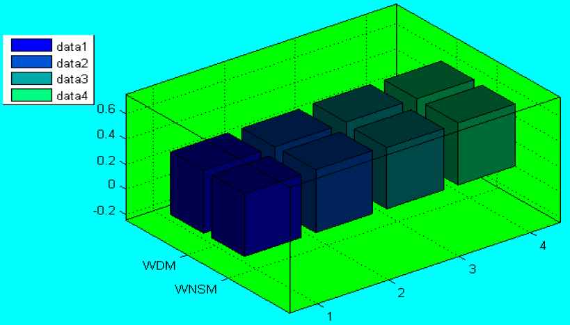
Figure 1

Geometrical expressions of the Example 2.

Step 3: The ranking results can be obtained as follows:

Because

ΨCI−3>ΨCI−4>ΨCI−1>ΨCI−2
Ψ′^CI−2>Ψ^′CI−1>Ψ′^CI−4>Ψ^′CI−3

So we can get the ranking orders of four alternatives shown as ℭCQ−2>ℭCQ−1>ℭCQ−4>ℭCQ−3.

From this ranking result, the TOPSIS based on WDM and WNSM obtained the same ranking result. In Example 2, the CQROFNs are used to express the evaluation information. Moreover, we choose the complex Pythagorean fuzzy information (CPFIs) and complex intuitionistic fuzzy information (CIFIs) to solve it by using the investigated measures. To discuss the above issues, we use the following examples.

Example 3.

To show the application of the investigated procedure in the environment of the MADM technique, we choose the real MADM example from Ref. [38]. Moreover, the needed information is discussed in Example 2. To resolve the above issue, we considered the weight vector for the attributes is demonstrated by: 0.4,0.3,0.2,0.1T, then the CPFIs are expressed shown in Table 3 (which are normalized). Based on the proposed TOPSIS, the steps of the developed decision-making procedure are given as follows.

Alternatives\Attributes PAt−1 PAt−2 PAt−3 PAt−4
ℭCQ−1 0.9ei2π0.8,0.1ei2π0.2 0.91ei2π0.81,0.11ei2π0.21 0.92ei2π0.82,0.12ei2π0.22 0.93ei2π0.83,0.13ei2π0.23
ℭCQ−2 0.85ei2π0.89,0.2ei2π0.1 0.86ei2π0.9,0.21ei2π0.11 0.87ei2π0.91,0.22ei2π0.12 0.88ei2π0.92,0.23ei2π0.13
ℭCQ−3 0.7ei2π0.8,0.3ei2π0.3 0.71ei2π0.81,0.31ei2π0.31 0.72ei2π0.82,0.32ei2π0.32 0.73ei2π0.83,0.33ei2π0.33
ℭCQ−4 0.85ei2π0.7,0.2ei2π0.3 0.86ei2π0.71,0.22ei2π0.32 0.87ei2π0.72,0.23ei2π0.33 0.88ei2π0.73,0.24ei2π0.34
Table 3

Normalized decision matrix with CPFIs.

Then by the investigated measures, the closeness indexes ΨCI−i and Ψ′CI−i are obtained as follows:

ΨCI−1=0.5009,ΨCI−2=0.4995,ΨCI−3=0.5052,ΨCI−4=0.5046
Ψ^′CI−1=0.4994,Ψ′^CI−2=0.5003,Ψ′^CI−3=0.4961,Ψ^′CI−4=0.4968

The calculated values are demonstrated in Figure 2. fig 2
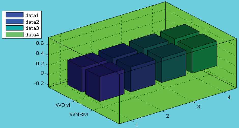
Figure 2

Geometrical expressions of Example 3.

Next, the ranking results can be obtained as follows:

Because

ΨCI−3>ΨCI−4>ΨCI−1>ΨCI−2
Ψ′^CI−2>Ψ^′CI−1>Ψ′^CI−4>Ψ^′CI−3

So we can get the ranking orders of four alternatives shown as

ℭCQ−2>ℭCQ−1>ℭCQ−4>ℭCQ−3

There are the same ranking results by WDM and WNSM, and the best alternative is ℭCQ−2. In Example 3, we used the CPFIs to resolve this problem by investigated measures. Moreover, we choose the complex intuitionistic fuzzy information (CIFIs) to resolve this problem.

Example 4.

To show the application of the investigated procedure in the environment of the MADM technique, we choose the real MADM example from Ref. [38]. Moreover, the needed information is discussed in Example 2. To resolve this problem, we considered the weight vector for the attributes is 0.4,0.3,0.2,0.1T, then the CIFIs are expressed shown in Table 4 (which are normalized). Based on the proposed TOPSIS, the steps of the developed decision-making procedure are given as follows.

Alternatives\Attributes PAt−1 PAt−2 PAt−3 PAt−4
ℭCQ−1 0.7ei2π0.6,0.1ei2π0.2 0.71ei2π0.61,0.11ei2π0.21 0.72ei2π0.62,0.12ei2π0.22 0.73ei2π0.63,0.13ei2π0.23
ℭCQ−2 0.6ei2π0.8,0.2ei2π0.1 0.61ei2π0.81,0.21ei2π0.11 0.62ei2π0.82,0.22ei2π0.12 0.63ei2π0.83,0.23ei2π0.13
ℭCQ−3 0.5ei2π0.5,0.3ei2π0.3 0.51ei2π0.51,0.31ei2π0.31 0.52ei2π0.52,0.32ei2π0.32 0.53ei2π0.53,0.33ei2π0.33
ℭCQ−4 0.7ei2π0.4,0.2ei2π0.3 0.71ei2π0.41,0.22ei2π0.32 0.72ei2π0.42,0.23ei2π0.33 0.73ei2π0.43,0.24ei2π0.34
Table 4

Normalized decision matrix with CIFIs.

The calculated values are demonstrated in Figure 3.

Then by the investigated measures, the closeness indexes ΨCI−i and Ψ′CI−i are obtained as follows.
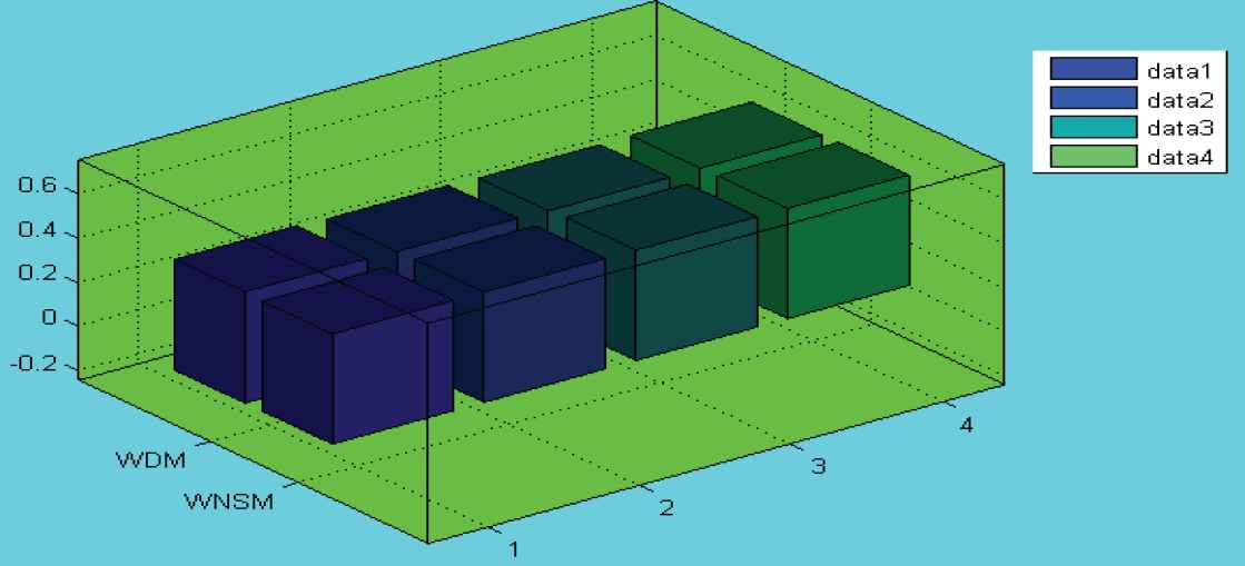
ΨCI−1=0.5051,ΨCI−2=0.4981,ΨCI−3=0.4937,ΨCI−4=0.4973
Ψ′^CI−1=0.4996,Ψ^′CI−2=0.5002,Ψ′^CI−3=0.5007,Ψ′^CI−4=0.5003
Figure 3

Graphical expressions of Example 4.

Then the ranking results can be obtained as follows:

Because

ΨCI−1>ΨCI−2>ΨCI−4>ΨCI−3
Ψ′^CI−3>Ψ^′CI−4>Ψ′^CI−2>Ψ^′CI−1

So we can get the ranking orders of four alternatives shown as

ℭCQ−3>ℭCQ−4>ℭCQ−2>ℭCQ−1

There are the same ranking results by WDM and WNSM, and the best alternative is ℭCQ−3. Therefore, the investigated measures based on CQROFSs are extensively useful to process complex data.

5. COMPARATIVE ANALYSIS

To show the validity and capability of the presented approach, we can compare it with some existing methods discussed as follows: Ye [41] developed CSMs based on IFSs, Mohd and Abdullah [42] explored CSMs for PFS, Liu et al. [38] presented CSMs for QROFSs, Garg and Rani [37] investigated the SMs for CIFSs, and Ullah et al. [27] explored DMs for CPFSs. By Example 2, the comparative analysis is shown in Tables 5 and 6.

Methods Score Values/Measures Values Ranking Values
Ye [41] Cannot resolve it Cannot resolve it
Mohd and Abdullah [42] Cannot resolve it Cannot resolve it
Liu et al. [38] Cannot resolve it Cannot resolve it
Garg and Rani [37] Cannot resolve it Cannot resolve it
Ullah et al. [27] Cannot resolve it Cannot resolve it
Proposed WDM ΨCI−1=0.5,ΨCI−2=0.4986,ΨCI−3=0.5064,ΨCI−4=0.5031 ℭCQ−2>ℭCQ−1>ℭCQ−4>ℭCQ−3
Table 5

Comparative analysis of the proposed and existing distance measures.

Methods Score Values/Measures Values Ranking Values
Ye [41] Cannot resolve it Cannot resolve it
Mohd and Abdullah [42] .. Cannot resolve it
Liu et al. [38] Cannot resolve it Cannot resolve it
Garg and Rani [37] Cannot resolve it Cannot resolve it
Ullah et al. [27] Cannot resolve it Cannot resolve it
Proposed WNSM Ψ′^CI−1=0.5,Ψ′^CI−2=0.5019,Ψ′^CI−3=0.4886,Ψ′^CI−4=0.4954 ℭCQ−2>ℭCQ−1>ℭCQ−4>ℭCQ−3
Table 6

Comparative analysis of the proposed and existing ideas for similarity measures.

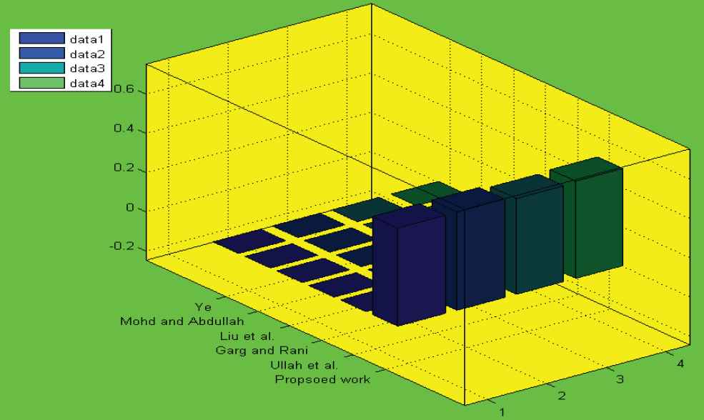
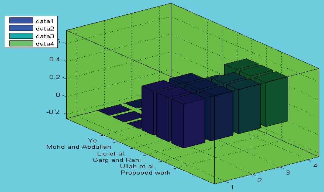
The calculated values in Tables 5 and 6 are demonstrated in Figures 4 and 5.
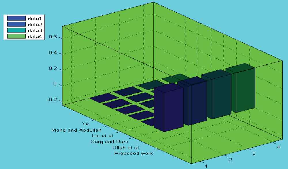
Figure 4

Geometrical expressions of Table 5.

Figure 5

Geometrical expressions of Table 6.

Figures 4 and 5 contain graphical expressions of six different types of measures, and each measure contains four alternatives.

Based on the information of Example 3, the comparative analysis of the presented method with some existing methods is discussed in Tables 7 and 8.

Methods Score Values/Measures Values Ranking Values
Ye [41] Cannot resolve it Cannot resolve it
Mohd and Abdullah [42] Cannot resolve it Cannot resolve it
Liu et al. [38] Cannot resolve it Cannot resolve it
Garg and Rani [37] Cannot resolve it Cannot resolve it
Ullah et al. [27] ΨCI−1=0.6171,ΨCI−2=0.6003,ΨCI−3=0.6278,ΨCI−4=0.6189 ℭCQ−2>ℭCQ−1>ℭCQ−4>ℭCQ−3
Proposed WDM ΨCI−1=0.5009,ΨCI−2=0.4995,ΨCI−3=0.5052,ΨCI−4=0.5046 ℭCQ−2>ℭCQ−1>ℭCQ−4>ℭCQ−3
Table 7

Comparative analysis of the proposed and existing distance measures.

Methods Score Values/Measures Values Ranking Values
Ye [41] Cannot resolve it Cannot resolve it
Mohd and Abdullah [42] Cannot resolve it Cannot resolve it
Liu et al. [38] Cannot resolve it Cannot resolve it
Garg and Rani [37] Cannot resolve it Cannot resolve it
Ullah et al. [27] Ψ^CI−1=0.3829,Ψ^CI−2=0.3997,Ψ^CI−3=0.3722,Ψ^CI−4=0.3811 ℭCQ−2>ℭCQ−1>ℭCQ−4>ℭCQ−3
Proposed WNSM Ψ′^CI−1=0.4994,Ψ′^CI−2=0.5003,Ψ′^CI−3=0.4961,Ψ′^CI−4=0.4968 ℭCQ−2>ℭCQ−1>ℭCQ−4>ℭCQ−3
Table 8

Comparative analysis of the proposed and existing ideas for similarity measures.

For the existing measures, we choose another set: ℭCQ=1ei2π1,0.0ei2π0.0,1ei2π1,0.0ei2π0.0,1ei2π1,0.0ei2π0.0,1ei2π1,0.0ei2π0.0, then

The calculated values in Table 7 are demonstrated in Figure 6.
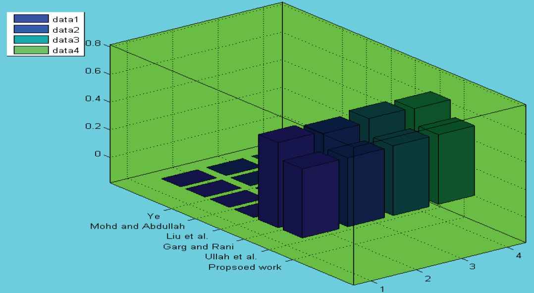
Figure 6

Graphical expressions of Table 7.

The calculated values in Table 8 are demonstrated in Figure 7.
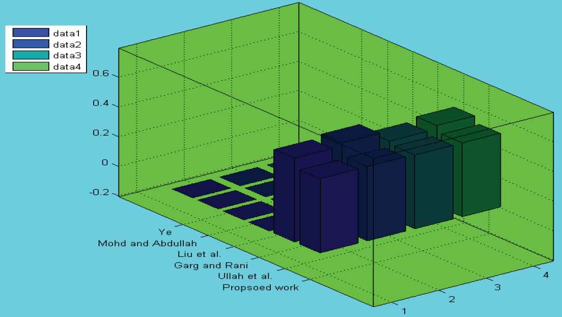
Figure 7

Graphical expression of Table 8.

Figures 6 and 7 contain graphical expressions of six different types of measures, and each measure contains four alternatives.

Based on the information of Example 4, the comparative analysis of the presented method with some existing methods is discussed in Tables 9 and 10.

Methods Score Values/Measures Values Ranking Values
Ye [41] Cannot resolve it Cannot resolve it
Mohd and Abdullah [42] Cannot resolve it Cannot resolve it
Liu et al. [38] Cannot resolve it Cannot resolve it
Garg and Rani [37] Ψ^CI−1=0.5038,Ψ^CI−2=0.4978,Ψ^CI−3=0.3926,Ψ^CI−4=0.4955 ℭCQ−3>ℭCQ−4>ℭCQ−2>ℭCQ−1
Ullah et al. [27] Ψ^CI−1=0.5115,Ψ^CI−2=0.4991,Ψ^CI−3=0.5043,Ψ^CI−4=0.5025 ℭCQ−2>ℭCQ−4>ℭCQ−3>ℭCQ−1
Proposed WDM ΨCI−1=0.5051,ΨCI−2=0.4981,ΨCI−3=0.4937,ΨCI−4=0.4973 ℭCQ−3>ℭCQ−4>ℭCQ−2>ℭCQ−1
Table 9

Comparative analysis of the proposed and existing distance measures.

Methods Score Values/Measures Values Ranking Values
Ye [41] Cannot resolve it Cannot resolve it
Mohd and Abdullah [42] Cannot resolve it Cannot resolve it
Liu et al. [38] Cannot resolve it Cannot resolve it
Garg and Rani [37] Ψ^CI−1=0.4985,Ψ^CI−2=0.4991,Ψ^CI−3=0.4998,Ψ^CI−4=0.4993 ℭCQ−3>ℭCQ−4>ℭCQ−2>ℭCQ−1
Ullah et al. [27] Ψ^CI−1=0.4991,Ψ^CI−2=0.4997,Ψ^CI−3=0.5002,Ψ^CI−4=0.4999 ℭCQ−3>ℭCQ−4>ℭCQ−2>ℭCQ−1
Proposed WNSM Ψ′^CI−1=0.4996,Ψ′^CI−2=0.5001,Ψ′^=0.5007,Ψ^CI−4=0.5003 ℭCQ−3>ℭCQ−4>ℭCQ−2>ℭCQ−1
Table 10

Comparative analysis of the proposed and existing similarity measures.

The ranking order produced by Ullah et al. [27] is different from the others.

The calculated values in Tables 9 and 10 are demonstrated in Figures 8 and 9.
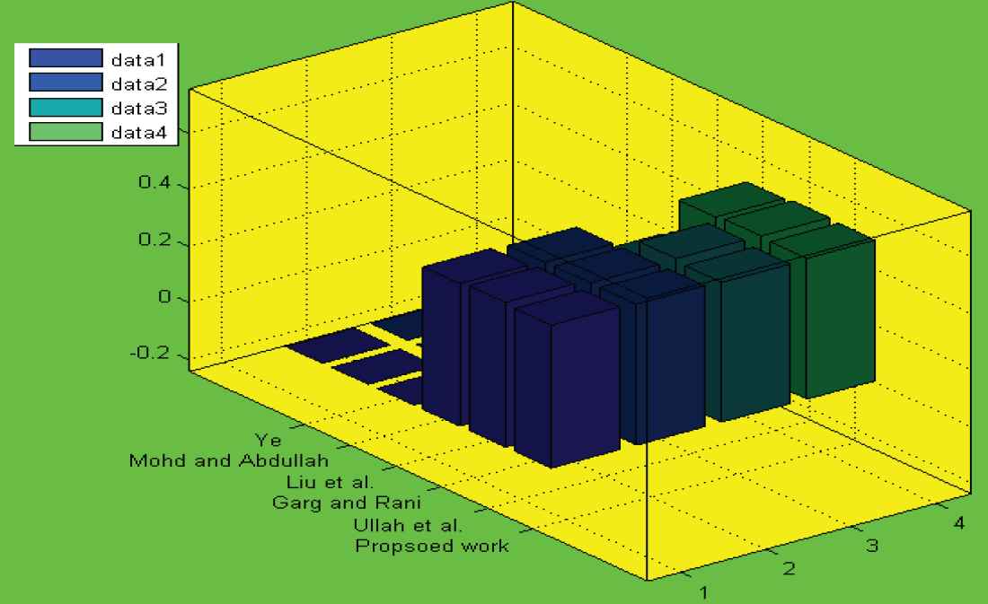
Figure 8

Geometrical expressions of Table 9.

Figure 9

Geometrical expressions of Table 10.

Figures 8 and 9 contain graphical expressions of six different types of measures, and each measure contains four alternatives.

From the above discussions, we obtain that if we choose the CQRIFIs, then the existing measures based on CIFSs, CPFSs are their special cases based on Tables 5–10. Therefore, the investigated measures based on CQROFSs are more general and useful to solve the MADM problem with complex uncertain information.

6. CONCLUSION

As a modification of the QROFSs, CQROFSs are an important and useful tool to describe the complex inaccurate information by complex-valued truth grades with an additional term, named as phase term. CSMs and DMs are an important tool to verify the grades of similarity and discrimination between the two sets. In this manuscript, we develop some CSMs and DMs for CQROFSs. Then based on CSMs and EDMs of CQROFSs, we propose an extended TOPSIS method to solve the MADM problems. Finally, we provide some examples to demonstrate the practicality and efficiency of the suggested procedure. The graphical representations of the developed measures are also utilized in this manuscript.

The proposed work is more powerful than the existing ones such as IFSs, CIFSs, PFSs, CPFSs, and QROFSs. In the future, In the future, we will also extend some ideas [39,40,43,44] for complex QROFSs, or for some consensus-based extensions, we will extend the proposed ideas to complex spherical FSs [45] and complex T-spherical FS [46]. We will also develop some new MADM methods based on the proposed CSMs and EDMs for CQROFSs.

CONFLICTS OF INTEREST

The authors declare they have no conflicts of interest.

AUTHORS' CONTRIBUTIONS

Peide Liu: Conceptualization, Formal analysis, Data curation, Fund, Supervision, Writing review & editing. Zeeshan Ali: Conceptualization, Formal analysis, Investigation, Visualization, Project administration, Writing – original draft. Tahir Mahmood: Supervision, Validation, Software, Writing – review & editing.

ACKNOWLEDGMENTS

This paper is supported by the National Natural Science Foundation of China (No. 71771140), Project of cultural masters and “the four kinds of a batch” talents, the Special Funds of Taishan Scholars Project of Shandong Province (No. ts201511045), Major bidding projects of National Social Science Fund of China (No. 19ZDA080).

REFERENCES

Journal
International Journal of Computational Intelligence Systems
Volume-Issue
14 - 1
Pages
1653 - 1671
Publication Date
2021/06/10
ISSN (Online)
1875-6883
ISSN (Print)
1875-6891
DOI
10.2991/ijcis.d.210528.002How to use a DOI?
Copyright
© 2021 The Authors. Published by Atlantis Press B.V.
Open Access
This is an open access article distributed under the CC BY-NC 4.0 license (http://creativecommons.org/licenses/by-nc/4.0/).

Cite this article

TY  - JOUR
AU  - Peide Liu
AU  - Zeeshan Ali
AU  - Tahir Mahmood
PY  - 2021
DA  - 2021/06/10
TI  - Some Cosine Similarity Measures and Distance Measures between Complex q-Rung Orthopair Fuzzy Sets and Their Applications
JO  - International Journal of Computational Intelligence Systems
SP  - 1653
EP  - 1671
VL  - 14
IS  - 1
SN  - 1875-6883
UR  - https://doi.org/10.2991/ijcis.d.210528.002
DO  - 10.2991/ijcis.d.210528.002
ID  - Liu2021
ER  -