
Comparing Circular Histograms by Using Modulo Similarity and Maximum Pair-Assignment Compatibility Measure
- DOI
- 10.2991/ijcis.2017.10.1.1How to use a DOI?
- Keywords
- Circular histograms; similarity; Łukasiewicz logic; Similarity; Modulo similarity; Compatibility
- Abstract
Histograms are an intuitively understandable tool for graphically presenting frequency data that is available for and useful in modern data-analysis, this also makes comparing histograms an interesting field of research. The concept of similarity and similarity measures have been gaining in importance, because similarity and similarity measures can be used to replace the simpler distance measures in many data-analysis applications. In this paper we concentrate on circular histograms that are well-suited for time or direction-stamped frequency data and especially on the comparison of circular histograms by way of similarity. We focus on Łukasiewicz many-valued logic based similarities and introduce a new similarity measure, the “modulo similarity” for circular problems. We prove that modulo similarity is a similarity measure in the strict sense. We also present a new compatibility measure, the “maximum pair assignment compatibility” that can be used in lossless sample-based comparison of histograms. We demonstrate the usefulness of these two new concepts by numerically applying them to a comparison of circular histograms and comparatively analyze the results with results from a comparison with a bin-based Łukasiewicz many-valued logic based method for the comparison of histograms.
- Copyright
- © 2017, the Authors. Published by Atlantis Press.
- Open Access
- This is an open access article under the CC BY-NC license (http://creativecommons.org/licences/by-nc/4.0/).
1. Introduction
This paper concentrates on the problem of comparing histograms and more specifically focuses on the comparison of circular histograms. Histograms are a well-known graphical representation of frequency data that allows intuitive understanding of the data. “Circular problems” are situations, where information is naturally represented in a circular way, examples include, temporal problems (clock-face) and directional problems (compass-face). In cases, where direction or time-stamped frequency information is available, circular histograms can be used. The difference between normal and circular problems is that where extremes of a scale, e.g., histogram bins, in a normal situation are the furthest apart from each other, in a circular problem they are respectively next to each other.
Histograms are used in a wide variety of applications and their usage is likely to increase in the future. One area of research related to histograms is the comparison of histograms. Comparison of histograms is by no means a trivial task, because when histograms are being compared the type of histogram used, normal (horizontal) or circular, must be taken into consideration.
A common approach in the comparison of histograms is to compute a distance between histograms by using one of many different distance measures.1 One possible way to do this is to first transform the histograms into a probability density functions (PDF) and to then compare these. This PDF-based approach was one of the first ones introduced for comparing histograms, and is based on the assumption that a histogram from measured values provides the basis for an empirical estimate of the PDF.2 Bhattacharyya distance (sometimes referred to as B-distance) is among the first distance measures used for calculating the distance between two statistical populations3; later on also other distance measures have been applied to the comparison of PDFs, e.g., the K-L distance4 being one of the first ones.
In what can be called “vector type of approaches”, histograms are treated as fixed-dimensional vectors, between which a distance is computed. The usually applied distance measures include the Euclidean and the Manhattan distances, or generalizations of these, like the Minkowski distance, see Ref. 5 for a listing of different types of distances and generalizations of standard Euclidean and Manhattan distances. Intersectional approaches consider the overlapping / non-overlapping parts of histograms as a basis for the comparison, these methods also use distances, e.g., earth mover’s distance6 and the idea is that the distance is based on computing the minimal amount of work required to transform one histogram into the other by moving “distribution mass”.
Angular separation and correlation functions are often applied in astrophysics, e.g., see Ref. 7, when histograms are compared. Also, in laser scans histogram correlation is sometimes used8. Chord distribution9,10 is also one way of comparing histograms that is often applied in literature. In this research we concentrate on a Łukasiewicz many-value logic based approach for comparing histograms, see Ref. 11, and leave other approaches outside the focus of this paper.
Comparison of histograms can be done by using a similarity measure instead of using a distance measure. In this paper we further focus on using similarity in the comparison of histograms. The notion of similarity is essentially a generalization of the notion of equivalence, more concretely one can say that a “similarity” relation S, is a fuzzy relation, which is reflexive, symmetric, and transitive.12 In the case that a relation fails to satisfy the condition of transitivity and thus is not a similarity, it is often referred to as a “compatibility”, or a “tolerance” relation.13 Searching through the literature, one can find that several measures that are called “similarity measures” are in reality only reflexive and symmetric, see Refs. 14–16; the definition of a “similarity measure” seems to be imprecise or fuzzy. In fact, several studies (see, e.g., Refs 17–19) show that similarity measures do not necessarily have to be transitive. Since the concept of similarity is a generalization of the notion of equivalence, we can even go as far as to say that first similarity measures were introduced by researchers working on many-valued logic. An excellent short introduction into the history of many-valued logic is given in Ref. 20.
We focus on Łukasiewicz many-valued logic21 based similarities and examine how these similarity measures can be used in the comparison of histograms. In this vein, we introduce a new similarity measure that we call “modulo similarity” and that is based on Łukasiewicz many-valued logic. We also introduce a new compatibility measure that we call “maximum pair assignment compatibility” (MPAC) that is useful in determining the similarity of histograms in terms of sample value similarity by considering the maximum pair assignment between two samples. An observed benefit of this sample value similarity based comparison is that there is no information loss in the comparison between samples of the same size. Both, modulo similarity measure and the maximum pair assignment compatibility measure are recent contributions and they have not been previously analyzed in detail.
This paper continues as follows: in section 2, we give a presentation of different histogram types and present the concept of similarity between histograms. We introduce the new modulo similarity measure for circular problems and present its axiomatic properties. Furthermore, we introduce the new maximum pair assignment compatibility measure (MPAC) and study also its axiomatic properties.
In section 3, a number of numerical illustrations are presented to show the usability of the new concepts in practice. In section 4, we show how the new methods compare with a Łukasiewicz many-valued logic based histogram comparison method that is based on bin comparison. Futhermore, we illustrate how one can overcome problems with histograms with different sample sizes, and observe some benefits and shortcomings of MPAC. Section 5 closes the paper with discussion and conclusions.
2. Similarity of histograms
In order to share light on why modulo similarity is useful and what are the reasons for which it should be applied in the comparison of circular histograms we first start with the definition of a histogram. We also go through the requirements for a lossless representation of histograms, because it is relevant for the lossless comparison of histograms MPAC. After this we move onto presenting different types of histograms, and how to define the similarity between histograms.
Definition 1.
Let x be a feature having m different values given in a set X = {x1,…,xm}. Consider set of elements A = {a1,…,an} where aj ∈ X. The histogram of the set A along with feature x is H(x,A) giving an ordered m-dimensional list consisting of the number of occurrences of the discrete values of x among ai.
Here we focus in the comparison of histograms of the same measurement x, a situation relevant when “standard” frequency data sets are being compared, notation H(A) will be used. If Hi(A), 1 ≤ i ≤ m, denotes the number of elements of A that have values xi, then (A) = {H1(A), H2(A),…,Hm(A)}, where
Note: If Pi(A) denotes the probability of samples in the jth value, then
Definition 2.
Lossless histogram representation:
Let x be a feature having m different values given in a set X = {x1,…,xm} and consider set of elements A = {a1,…,an} where aj ∈ X. Histogram H(A) (or HP(A), if using (2)) and number of bins equaling m presents lossless histogram representation of A.
Example 1.
Consider n=10, m=6 and A={1,6,5,1,1,2,5,5,1,1}, H(A)={5,1,0,0,3,1}, and HP(A)={0.5,0.1,0,0,0.3,0.1}. If the ordering of the elements in the set A is not considered, then H(A) is a lossless representation of A, meaning that A can be fully reconstructed from H(A). Notice that if we introduce requirement that m<6 this reconstruction cannot be done anymore.
2.1. Different histogram types
Histograms can be divided into three different types, in connection with computing histogram similarities: 1) nominal, 2) ordinal, and 3) circular.
In nominal histograms each variable has a “name” that is, “make of a car” can take nominal values such as “Volvo”, “Saab”, “Tesla”, and so forth. Nominal type histograms can, e.g., consist of the frequency of each make of car in a parking lot. In ordinal type histograms, the variables are (can be) ordered, e.g., the number of valves in a car can be quantified into 2 to 5 valves per cylinder, or the weight of the vehicle from 1 to 10 tons and these can be ordered.
In the third, circular type histograms, the measured (or observed) variables form a circle in the same way as hours form a circle on a clock-face with arithmetic modulo 12, or a compass with degrees arithmetic modulo 360. Ordinal and circular histograms are illustrated in Figure 1.
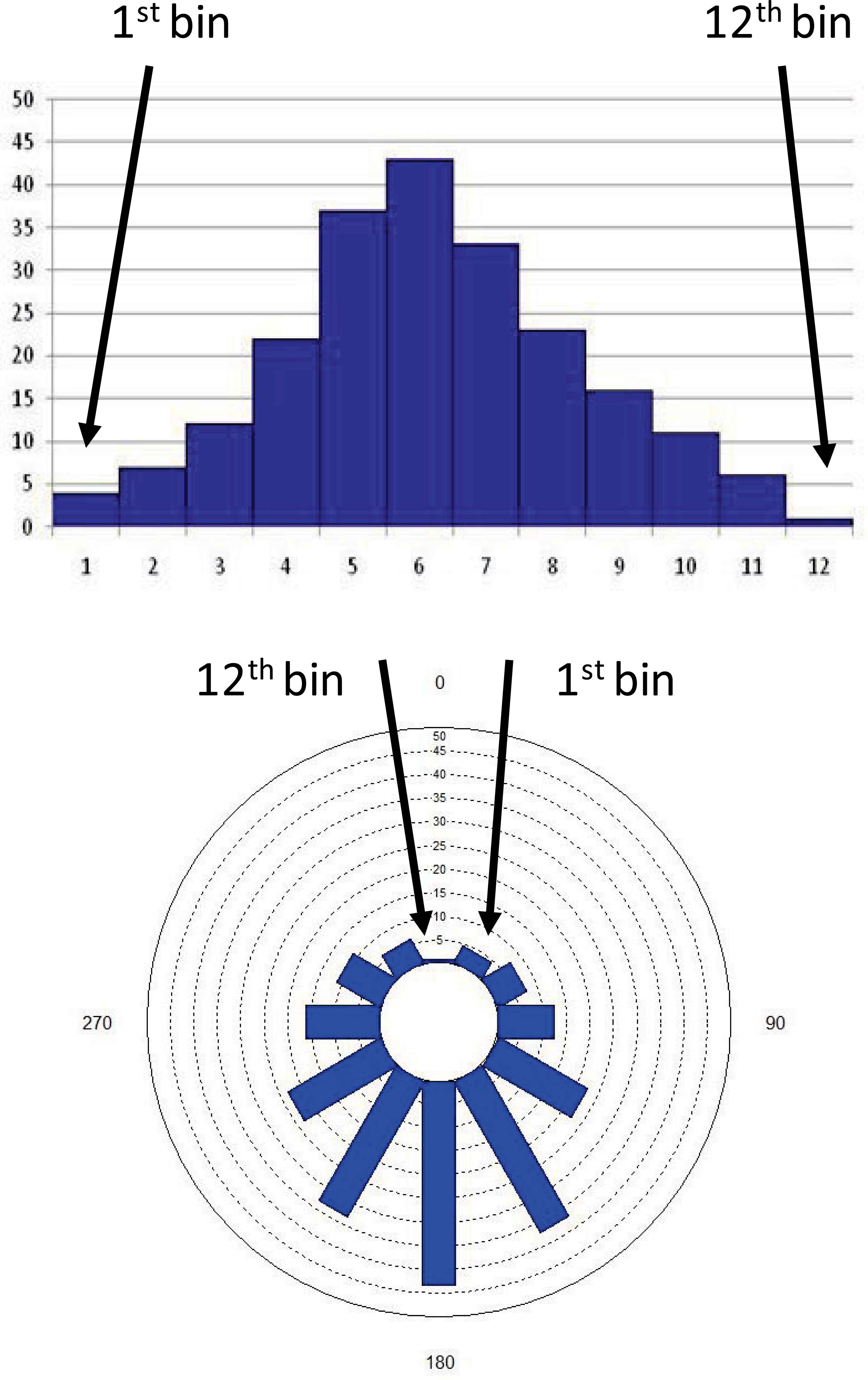
An ordinal and a circular histogram of the same frequency information. The first bin in the circular histogram is at a 30°angle, next to the 12th bin at 360°/0° angle, while in the ordinal histogram the 1st and the 12th bin are the furthest apart.
2.2. Similarity between samples from discrete measurements
Given a set of samples, with each sample containing measured discrete values of a variable, a histogram represents the frequency of each discrete variable value measured. Considering three different types of measurements, nominal, ordinal, and circular (modulo), we present three different similarities between two measurements (samples) xa, xb ∈ X. We normalize the sample values between unit intervals, by setting
Nominal similarity:
Where, for the similarity of two nominal type sample values, we either have a match, or we don’t, this is in line with classical equivalence.
Ordinal similarity:
Where the similarity of the element values is defined in the same way as in the original Łukasiewicz similarity [15, 16].
Modulo similarity:
Where, the values form a circle and the form must be taken into consideration, when the similarity is calculated.
2.3. Similarity in the Łukasiewicz structure and axiomatic properties of modulo similarity
Since, in (4) and (5) we are using similarity based on Łukasiewicz many-valued logic, let us first start by brief review of axiomatic properties required for this similarity. Also note that our first equation for similarity (3) is same as the standard crisp equivalence relation. To be a similarity measure in the strict sense, as discussed above, a Łukasiewicz similarity measure21 needs to satisfy the conditions of reflexivity, symmetricity, and transitivity. Since Łukasiewicz structure can be defined by residuated lattice, we first start by introducing definitions for a lattice and a residuated lattice, then we present the Łukasiewicz structure and Łukasiewicz similarity. In definitions 3–6 we follow closely the work of Turunen, see Ref 20.
Definition 3.
A lattice is partially ordered set in which x ∧ y (infimum) and x ∨ y(supremum) exists in L for all elements x, y ∈ L. A lattice is often denoted by 〈L, ≤,∧,∨〉.
Definition 4.
A lattice is called residuated, if it contains the greatest element 1, and binary operations ⊙ (called multiplication) and → (called residuum) such that following conditions hold
- 1.
⊙ is associative, commutative, and isotone.
- 2.
a ⊙ 1 = a for all elements a ∈ L and
- 3.
for all elements a, b, c ∈ L, a ⊙ b ≤ b if and only if a ≤ b → c
Definition 5.
Letting L be the real unit interval [0,1] endowed with the usual order relation, we may construct the following usual residuated lattice: Łukasiewicz structure: a ⊙ b = max{a + b − 1,0}, a → b = min{1,1 − a + b}.
Definition 6.
Let L be a residuated lattice and X is a non empty set. L-valued binary relation S, defined in X is a similarity if it fulfills the following conditions:
- 1.
∀x ∈ X: S(x, x) = 1
- 2.
∀x1, x2, ∈ X: S(x1, x2) = S(x2, x1)
- 3.
∀x1, x2, x3, ∈ X: S(x1, x2)⊙S(x2, x3) ≤ S(x1, x3)
Notice that in case we let L be the two element set {0,1}, similarity coincides with the usual equivalence relation, see nominal similarity eq. (3). In Łukasiewicz-logic an equivalence relation (or similarity relation) is defined as 1 − max{x1, x2} + min{x1, x2}, or equivalently as S(x1, x2) = 1 − |x1 – x2|, see Ref. 15 and also ordinal similarity eq. (4).
Next we provide theorem that the new modulo similarity is reflexive, symmetric and transitive (conditions 1, 2, and 3 in definition 6) and provide proofs for these in the Appendix.
Theorem 1.
Modulo Smod satisfies reflexivity, symmetricity and transitivity (see proofs in Appendix A).
Because all three axioms hold, we conclude that modulo similarity is a similarity measure in the sense defined by Łukasiewicz21 and satisfies the conditions of reflexivity, symmetricity, and transitivity.
2.4. Maximum pairwise assignment compatibility (MPAC) measure and its axiomatic properties
The similarity between any two histograms can be given in terms of sample value similarities. Given two samples of n elements, A and B we approach this problem by considering maximum similarity of pair assignments between the two samples. The problem is to determine the best one-to-one assignment between the two samples, such that the mean of all similarities between two individual elements in a pair is maximized. Given m elements ai ∈ A, and m elements bi ∈ B, we define the maximum pair assignment compatibility (MPAC) as:
Definition 6.
Given A = {a1,…,an} and B = {b1,…,bn} where aj ∈ X, bj ∈ X, and m different bins representing all possible feature values in a set X = {x1,…,xm}. Normalized values for A and B are
To get a better understanding from S(Am, Bm) we next provide two theorems explaining its properties. Proofs of the theorems are given in the Appendix.
Theorem 2.
S(Am, Am) is non-negative.
Proof:
see Appendix A.
Theorem 3.
S(Am, Am) is reflexive and symmetric.
Proof.
see Appendix A.
Two of the three conditions that are the strict requirement for a similarity are fulfilled by the maximum pairwise compatibility measure.
3. Numerical illustrations of comparing histograms with the maximum pairwise compatibility measure
Next we illustrate, with a numerical example, how modulo similarity can be used with the maximum pair assignment compatibility measure to compare histograms of the same dimension (same m and n). Later we discuss what can be done, if these requirements are not met (e.g. different n), which often is the case in real world situations. We approach this topic by way of two different types of “attitudes”: 1) removal of samples from the larger set and by 2) interpolation of samples from the smaller set.
3.1. Comparing samples of same dimensions
In next example we assume the problem studied to be circular in nature and show how one can end up with different results by applying nominal, ordinal, and modular approaches. Consider the following three samples of observations with the same dimensions m=8 and n=10:
A={1,1,1,1,2,3,7,7,7,8},
B={1,2,2,2,2,3,7,7,7,8}, and
C={1,1,2,3,7,7,7,8,8,8}.
The corresponding histograms are:
H(A)={4,1,1,0,0,0,3,1},
H(B)={1,4,1,0,0,0,3,1}, and
H(C)={2,1,1,0,0,0,3,3}.
Applying the maximum pair assignment similarity to these cases we get:
Figure 2 shows the ordinal and circular histograms for the three sets of observations. And a summary of all the results by maximum pair similarity assignment is visible in Table 1.
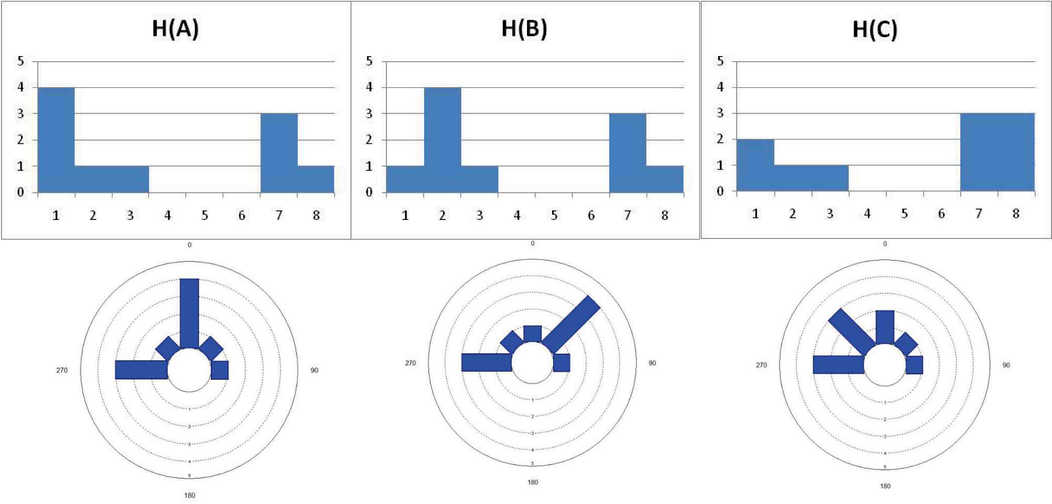
Ordinal and circular histograms H(A), H(B), and H(C)
| Pairs: | Snom | Sord | Smod |
|---|---|---|---|
| A,B | 0.7 | 0.963 | 0.963 |
| A,C | 0.8 | 0.825 | 0.975 |
| B,C | 0.7 | 0.838 | 0.938 |
Maximum pair assignment compatibilities for all the illustrated cases.
If we look at the calculation of the maximum pairwise compatibility between the histograms H(A) and H(C) and visualize the process by looking at the pairs of the observations “within” the histograms graphically, we get Figure 3, where similarity of each pair of observations is first calculated separately and then the sum of the similarities is added up and normalized to yield the maximum pairwise compatibility. It is easy to see from Figure 3 that there is a clear difference between the resulting maximum pairwise compatibilities when using nominal, ordinal, and modulo similarities for the “same data”. Usually we want to find the best possible match with histograms and higher similarity values are considered better. In Figure 3, we can see that nominal or ordinal similarity calculation gives low similarity values for samples without an exact match (s(1,8)=0 with nominal and (s(1,8)=0.125 with ordinal). It is however clear, that as this is a circular problem the sample pair (1,8) are adjacent and they should get high similarity (in the modulo similarity case we get s(1,8)=0.875), a high value). This demonstrates the advantage of using modulo similarity in MPAC for circular problems.
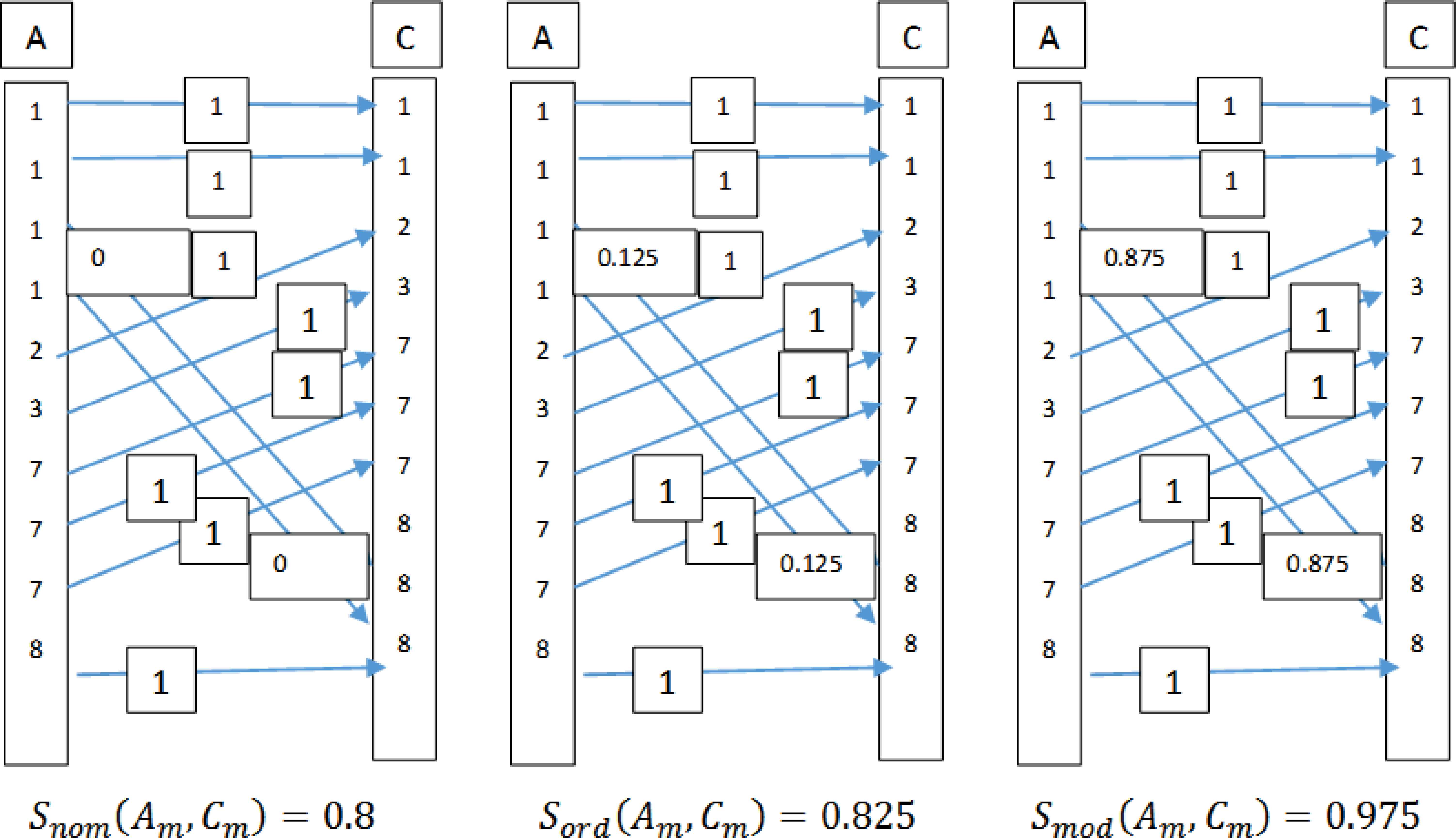
Maximum pairwise compatibility between H(A) and H(C) with, a) nominal similarity b) ordinal similarity and c) modulo similarity
3.2. Comparing samples with a different number of observations
The MPAC requires the sample sizes of the compared histograms to be equal, this is why we study the situation, where sample sizes are different and one must “artificially” make them equal.
The situation with different sample size that is, a different number of observations (sample values) can be considered as a missing data problem. Here we can address this problem by approaching it, e.g., in the following two ways: randomly deleting samples from the histogram with a larger number of samples, or by interpolating more sample values into the histogram with a smaller number of samples. In the first approach, the comparison of histograms can be done, e.g., by randomly selecting a min (nA, nB) amount of samples and calculating the similarity of histograms for histograms resulting from the smallest sample size. To get comprehensive results the procedure can be repeated several times and the average from these results can be used as (an indicator of) a compatibility score. An important issue to remember is that m is defined before the process.
When using an interpolation technique, one would interpolate max (nA, nB) -min (nA, nB) sample values to be added to the smaller set(s) with a lower number of sample values. We use probabilities of HP(A) or HP(B) in our interpolation. Next we shortly illustrate these procedures numerically.
Consider the following three samples with m=8 and nA=12, nB=15 nC=10:
A={1,1,1,1,2,3,4,4,7,7,7,8},
B={1,2,2,2,2,3,5,5,5,6,6,7,7,7,8},
C={1,1,2,3,7,7,7,8,8,8}.
Using random selection, ten sample values are selected from sets A and B. Then similarities and the maximum pairwise assignment compatibility (MPAC) measure values are calculated between the sets (in the same manner as in section 3.1). This procedure is then repeated 100 times and the mean MPAC measure value is computed for each pair of sets. The results of the mean MPAC measure values reached with the experiment are given in Table 2.
| Pairs: | Snom | Sord | Smod |
|---|---|---|---|
| A,B | 0.486 | 0.893 | 0.893 |
| A,C | 0.693 | 0.822 | 0.891 |
| B,C | 0.494 | 0.861 | 0.871 |
Mean maximum pairwise assignment compatibility measure values from 100 repetitions using random sampling, when nominal, ordinal, and modulo similarities are used.
For the example it seems that using nominal similarity with the MPAC leads to clearly lower MPAC values. Also the results between ordinal and modulo similarity are quite similar – in the example, both find the pair (A,B) as the closest match.
When interpolation is used, in this case three samples are created for and added to the set A and respectively five samples for the set C; this is done by using the frequencies presented in HP(A) and HP(C) as probabilities. In this way three sets of fifteen sample values become available. After the interpolation the maximum pairwise assignment compatibility is calculated between the three sets. This process is repeated 100 times and the mean similarities between the sets computed. The results of the mean MPAC values reached with the interpolation method are presented in Table 3. One can see that with ordinal similarity the pair (A,B) is considered to be the closest match, but with modulo similarity the MPAC finds the pair (A,C) the closest match. This result seems to indicate that modulo similarity does not perform as consistently as the nominal and ordinal similarity in situations, where the original number of samples in the to-be-compared histograms is not equal and when random deletion and/or interpolation are used.
| Pairs: | Snom | Sord | Smod |
|---|---|---|---|
| A,B | 0.533 | 0.890 | 0.899 |
| A,C | 0.665 | 0.807 | 0.906 |
| B,C | 0.555 | 0.862 | 0.893 |
Mean maximum pairwise assignment compatibility measure values from 100 repetitions using the interpolation method, when nominal, ordinal, and modulo similarities are used.
4. A bin-comparison based method in the comparison of histograms
Here we present an alternative Łukasiewicz many-valued logic based histogram bin comparison-based method for the comparison of histograms that is based on the “Turunen similarity”. This is done to highlight the benefits that can be obtained by using the MPAC with circular problems, and to demonstrate the difference between using a “sample comparison” based similarity technique to a “bin-based” comparison technique.
We analyze, by using numerical results from the two alternative methods, how different and what kind of differences exist between the selected methods and the maximum pairwise compatibility measure. First, we study the situation, where the compared histograms have same dimensions and then a situation where the dimensions are not the same – for both these cases we analyze the effect of using different number (and size) of bins. The idea is to create a benchmark for understanding the “goodness” and the usability of the MPAC and the Turunen similarity based method in practical circumstances.
4.1. Bin-based comparison of histograms with the same dimensions
We present a similarity measure that is usable for similarity computation of two histograms that is based on comparing bins, or in other words the number of observations in each bin. The comparison is done by comparing each bin to the corresponding bin on the compared-to histogram. This is done by using Łukasiewicz similarity that for the purposes of this research is called “Turunen similarity”, in the following way:
Definition 7.
Given two histograms HP(A) and HP(B) with m bins. Similarity of histograms S(HP(A), HP(B)) considering only m bins is:
This similarity measure is substantially the same as the similarity previously introduced by Turunen20, for the analysis of the axiomatic properties of this similarity measure we refer the interested reader to the original article. We consider the same histograms as in the previous illustration
H(A)={4,1,1,0,0,0,3,1},
H(B)={1,4,1,0,0,0,3,1}, and
H(C)={2,1,1,0,0,0,3,3}
HP(A)={0.4,0.1,0.1,0,0,0,0.3,0.1},
HP(B)={0.1,0.4,0.1,0,0,0,0.3,0.1}, and
HP(C)={0.2,0.1,0.1,0,0,0,0.3,0.3}.
| S(HP(A), HP(B)) | S(HP(A), HP(C)) | S(HP(B), HP(C)) |
|---|---|---|
| 0.925 | 0.925 | 0.925 |
Similarities of three histograms using equation (7) for Turunen similarity
One issue that needs to be noted here is that instead of pairwise sample comparison, the comparison is made for the bins. This means that the number (and the size) of bins matters.
This also means that there is information loss, if the number of bins used is reduced. In Figure 4, one can see how computed similarity values change, when the number of bins used is changed.
Similarities of histograms HP(A), HP(B) and HP(C) when quantity of bins are compared.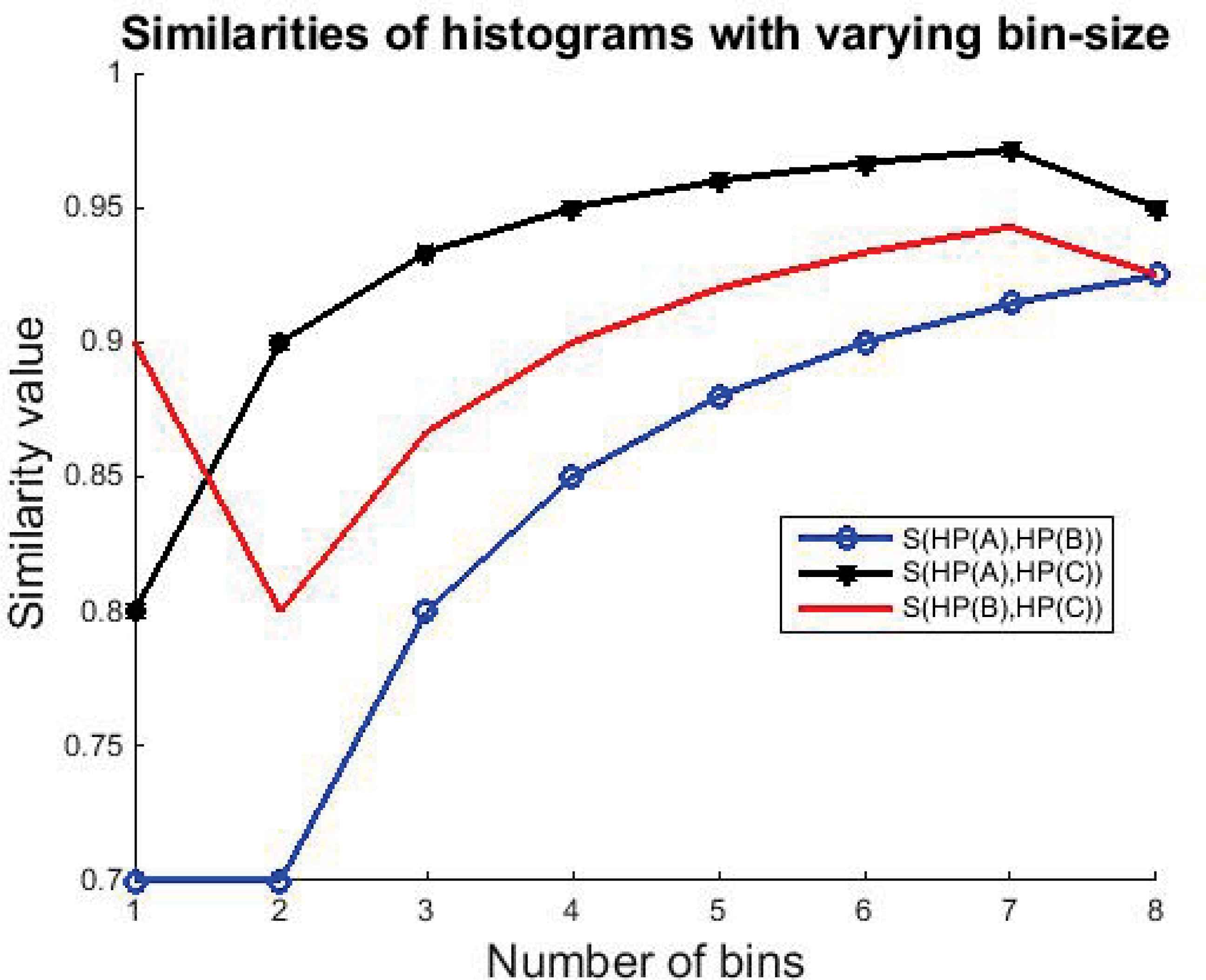
It is visible that even though the most common result for all studied quantities of bins is that histograms HP(A) and HP(C) are most similar, the bin size does affect the results. When only one bin was used the histograms HP(B) and HP(C) were found to bemost similar. When eight bins were used the similarity between the histograms HP(A) and HP(B) and with HP(B) and HP(C) “converged”. Furthermore, in the comparisons that are made based on the bins modularity is not taken into consideration in any way.
The obtained results suggest that the presented method that concentrates (only) on the bin size in the comparison of histograms is a more robust method than the MPAC.
4.2. Comparing histograms with different sample size (n)
In practice, one may encounter situations, where the number of collected samples is not the same for different sets (histograms). In such cases the need to introduce a general definition for histogram distributions with an arbitrary sample size arises. Let N = nA × nB, where nA and nB are the quantity of samples in sets A and B. A common multiplier for these would be N. Using a common multiplier we can derive new histograms HPN(A) and HPN(B), for comparison purposes in the following way:
After the derivation of the comparable histograms we can apply equation (7) in the calculation of similarities between histograms, where the number of samples are different. Consider again the following three cases, with m=8 and nA=12, nB=15, and nC=10:
A={1,1,1,1,2,3,4,4,7,7,7,8},
B={1,2,2,2,2,3,5,5,5,6,6,7,7,7,8},and
C={1,1,2,3,7,7,7,8,8,8}.
Corresponding derived comparable histograms are:
HPN(A)={0.33,0.083,0.083,0.17,0,0,0.25,0.083},
HPN(B)={0.07,0.27,0.07,0,0.2,0.13,0.2,0.07}, and
HPN(C)={0.2,0.1,0.1,0,0,0,0.3,0.3}.
The resulting similarities between the histograms with m=8 are given in Table 5.
|
|
|
|
|---|---|---|
| 0.9897 | 0.9925 | 0.9883 |
Similarities of three histograms by using normalization with a common multiplier
Testing the effect that changing the number of bins used has on the results gives us the results that are visible in Figure 5, where one can see that the number of bins used (bin size) has a clear effect on the similarity results.
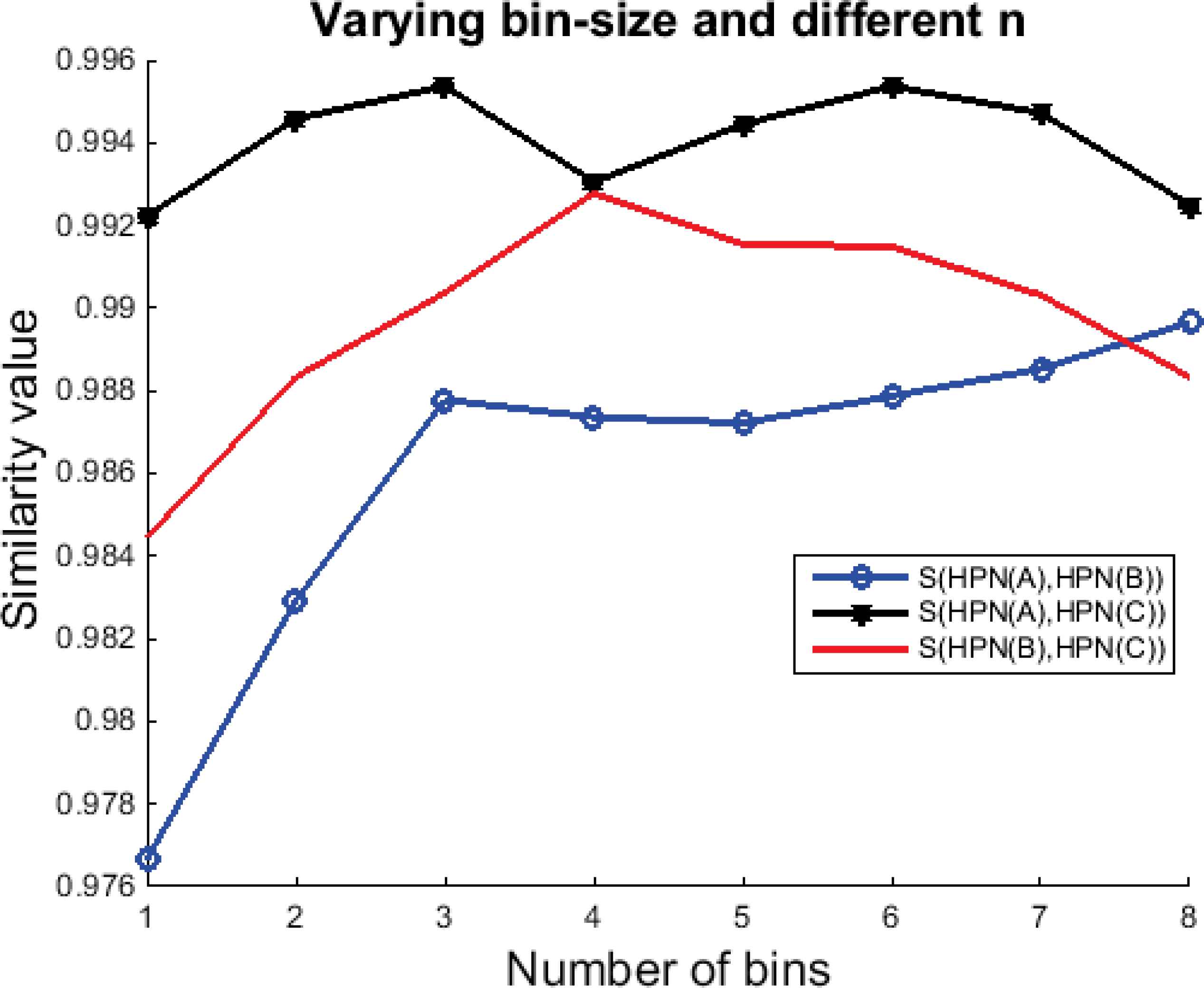
Similarities of histograms HPN(A), HPN(B), and HPN(C) when different quantity of bins are used.
Here we have shown how Łukasiewicz based similarities can be applied in the comparison of the histograms and examined how bin comparison-based comparison of histograms can be constructed by using the Łukasiewicz based Turunen similarity. To the best of our knowledge this is the first time the presented similarity is used for the comparison of histograms.
It was shown that the bin comparison-based similarity is simpler to use than the MPAC in cases, where histograms have different number of samples in the sense that they do not require random sampling or interpolation techniques to work. Shortcoming of the bin comparison-based method is that it does not specifically take into consideration the special circumstances of circular problems.
5. Discussion and conclusions
In this paper we have presented a new similarity measure, the “modulo similarity” and shown that it satisfies the three required axioms of a “true” similarity measure in the many-valued Łukasiewicz structure. We have also introduced a new method for comparing histograms based on pair-wise comparison of individual histogram bin-values that we call “maximum pair assignment compatibility” (MPAC) measure. The MPAC is a method that is based on comparing the individual samples from which the histograms are built, this is different from a bin-based comparison of histograms.
The MPAC method can utilize different types of similarity measures in the comparison of histograms, including using the new modulo similarity. We illustrated the use of the maximum pair assignment compatibility measure numerically by comparing histograms by using nominal, ordinal, and modulo similarities. When modulo similarity is used the MPAC is able to take into consideration the special properties of circular problems. It is clear that the presented new methods are relevant, when time-stamped, or direction-stamped information is used to form histograms.
An important advantage of the new method, over bin-based comparison of histograms, is the fact that more relevant information about the circular problems can be taken into consideration, which causes the results to be more realistic. Furthermore, the MPAC is a lossless procedure that is, as the comparison is performed based on the individual samples no information is lost in the process.
There are also issues that limit the use of the MPAC, or at least require solutions that may affect results. For example, the requirement to have equal sample size in the compared histograms may cause the need to equalize the sample sizes; some methods for achieving this were proposed and shortly illustrated.
We have also examined how a Łukasiewicz logic-based similarity (Turunen similarity) can be applied to comparing histograms. The method is based on comparing the bins of the histogram and to the best of our knowledge this is the first application of the method to comparison of histograms. The results from the Turunen similarity based method have been compared to the results from the MPAC and the findings show that bin-based comparison of histograms allows one to “directly” include cases, where two histograms have a unequal number of observations, however, the studied method cannot take into consideration circular problems.
So far, there has been little in terms of research of comparison of histograms in general and the research on circular histograms is scarce, even though it is quite apparent that there are many applications, where histograms are used and comparison of histograms is needed, as the amount of time- and direction-stamped data is all the time growing.
Future research into this topic will include, among other things, comparison of histograms from samples of fuzzy numbers and research into how the new methods may be used together with the histogram ranking method to compare the results from different parametric MCDM decision-support methods.
Appendix A.
Proof of theorem 1.
Reflexivity.
Symmetricity.
if
If
Transitivity.
Since we know that ∀x1, x2, ∈ X: S(x1, x2) = 1 – |x1, – x2| satisfies condition 3 (see, e.g., [16]) the proof reduces to a study of the cases, where also
- 1)
- 2)
- 3)
For 1) we have x1 ≤ x3 ≤ x2 and
Now,
In the case
Case
Since x2 ≤ x3, x2 – x3 ≤ 0, and we get 0 ≤ 0
In the case that we have x1 ≤ x3 ≤ x2, we get
Case
⇔ 0 ≤ 0
In the last case we have
in case
Since there are no other cases this concludes the proof
Proof of theorem 2.
Since s(ai, bj) ≥ 0 also sum
Proof of theorem 3.
Reflexivity.
For Am = Bm we have also ai = bj and since s(ai, ai) = 1 also in this case s(ai, bj) = 1 ∀ i, j. This leads to
Symmetricity.
Since s(ai, bj) = s(bj, ai) also
References
Cite this article
TY  - JOUR
AU  - Pasi Luukka
AU  - Mikael Collan
PY  - 2017
DA  - 2017/01/01
TI  - Comparing Circular Histograms by Using Modulo Similarity and Maximum Pair-Assignment Compatibility Measure
JO  - International Journal of Computational Intelligence Systems
SP  - 1
EP  - 12
VL  - 10
IS  - 1
SN  - 1875-6883
UR  - https://doi.org/10.2991/ijcis.2017.10.1.1
DO  - 10.2991/ijcis.2017.10.1.1
ID  - Luukka2017
ER  -