Observer based robust neuro-adaptive control of non-square MIMO nonlinear systems with unknown dynamics

Hassan Ghiti Sarand; Bahram Karimi

doi:10.2991/ijcis.2017.10.1.3

<Previous Article In Issue

Download article (PDF)

Next Article In Issue>

Volume 10, Issue 1, 2017, Pages 23 - 33

Observer based robust neuro-adaptive control of non-square MIMO nonlinear systems with unknown dynamics

Authors

Hassan Ghiti Sarand¹^,hghsarand@mut-es.ac.ir, Bahram Karimi¹^,bkarimi@mut-es.ac.ir

¹Department of Electrical Engineering, Malek Ashtar University of Technology, Shahin Shahr, Isfahan, Iran

Received 7 December 2015, Accepted 5 August 2016, Available Online 1 January 2017.

DOI: 10.2991/ijcis.2017.10.1.3 How to use a DOI?
Keywords: Non-square systems; Adaptive control; Observer; Neural network; Lyapunov stability
Abstract: This paper addresses a robust adaptive control problem of non-square nonlinear systems with unmeasurable states. The systems are assumed to be multi-input/multi-output subject to dynamical uncertainties and external disturbances. The approach is studied for two cases, i.e., underactuated and over-actuated nonlinear systems. The new observer does not need to satisfy the SPR conditions. Moreover, a constant full-rank matrix with an adaptive gain is used to approximate the unknown gain matrix. Therefore, the proposed controller’s structure simplifies its implementation. The unknown nonlinearity is estimated neural networks. Stability of the closed-loop system is proved using Lyapunov analysis. The feasibility of the proposed approach is validated by simulation examples.
Copyright: © 2017, the Authors. Published by Atlantis Press.
Open Access: This is an open access article under the CC BY-NC license (http://creativecommons.org/licences/by-nc/4.0/).

1. Introduction

In practice, many of physical systems are nonlinear multi-input/multi-output (MIMO) systems. Because of coupling between inputs and outputs, control of MIMO systems becomes a more complicated problem. One of the most important classes of nonlinear systems is high-order affine systems described as follows

(1)x(n)=f(x¯)+g(x¯)u+w(t)

where x = (x₁,…, x_m)^T ∈ R^m, x(n)=(x1(n1),…,xm(nm))T∈Rm . x¯=(x1,…,x1(n1−1),…,xm,…,xm(nm−1))T∈Rn , u ∈ R^p and w ∈ R^m are states, inputs and disturbances of the system, respectively. n=∑i=1mni is the state vector available for measurement. f(x) ∈ R^m is Lipschitz continuous vector function which represents the system dynamics and g(x) ∈ R^m×p is the input gain matrix. If m = p, the system is called a square or fully-actuated system while it is non-square for m ≠ p. Over-actuated systems have more inputs than outputs while in underactuated systems, number of inputs is less than outputs. The majority of the available researches focuses on controlling square type of unknown nonlinear MIMO systems and applies neural networks (NNs) or fuzzy logic models to approximate unknown nonlinearities, e.g. see Refs. 1–10. However, most of mechanical systems and chemical processes have non-square structure. Then, controller design for such systems becomes more challenging than their square counterparts. In Refs. 11–12, control of over-actuated multivariable nonlinear systems were studied. In Ref. 11 f(x) and g(x) were considered to be known while in Ref. 12 f(x) included unknown parameters. Fuzzy adaptive controllers for non-square nonlinear systems were introduced in Refs. 13–14. Two fuzzy models were used to estimate unknown dynamics and the input gain matrix and the stability analysis was only presented for over-actuated case. Moreover, several works were focused on control of underactuated nonlinear systems which have fewer control inputs than the degrees of freedom (DOF), e.g., Refs. 15–18. In Ref. 15 an adaptive fuzzy hierarchical sliding-mode control was proposed for single-input-multi-output uncertain nonlinear systems. In Ref. 16, an adaptive fuzzy sliding mode was considered for 2 DOF nonlinear systems. Aloui et al. addressed¹⁷ systems of equation (1) using a robust adaptive fuzzy controller. Due to the complex structure of the proposed control law, three fuzzy models were employed to approximate unknown dynamics and parameters. In Ref. 18, an adaptive sliding mode control scheme was proposed for underactuated affine nonlinear systems. In order to make the gain matrix square, slack variables were applied. Totally, a proper choice of slack variables to guarantee convergence of the closed-loop system is a challenging task.

According to the literature review, the proposed methods for control of nonlinear systems of equation (1) have employed two approximators such as NNs or fuzzy models to estimate unknown nonlinearities f(x) and g(x). Therefore, the number of adjustable parameters were increased considerably and resulted in complexity of the controller structure and increasing computational cost.

On the other hand, in many control problems, all the state variables are not available for direct measurement. In recent years, the design of adaptive control based on observer for uncertain nonlinear SISO systems has been developed broadly, e.g. see Refs. 19–25 and the references therein. While the problem is still a challenging task for unknown nonlinear MIMO systems. In Ref. 26, a neuro-sliding mode method combined to a state observer was introduced to control the system (1). In Ref. 27, using the strictly positive real (SPR) conditions on the estimation error dynamics, an observer-based adaptive fuzzy control was designed for nonlinear MIMO systems with constant input gain. In Ref. 28, an adaptive fuzzy robust controller was proposed for unknown systems of the equation (1) and a state observer was designed by using the SPR conditions. In order to satisfy the SPR conditions, a low-pass filter must be applied to augment observation error dynamics which results in the filtering of the fuzzy or NN basis functions and the other terms of the controller. Thus, these methods increase dynamic order of the controller or the observer considerably. Du and Qu proposed²⁹ an observer-based indirect adaptive controller for time delayed version of the system (1) but stability analysis was not presented. In Ref. 30, a high gain disturbance observer-based control was suggested for nonlinear affine systems with known dynamics. In Ref. 31, an observer-based adaptive fuzzy sliding mode control was designed for the system (1). But for the observer implementation, it is necessary all the states to be available for measurement. Then, the controller proposed in Ref. 31 is not realizable. The schemes proposed in Refs. 26–31 have considered the square nonlinear system.

In this paper, an observer based robust neuro-adaptive control method is proposed for non-square nonlinear systems of the equation (1) with unknown nonlinearities and subject to uncertain external disturbances. Instead of the gain matrix estimation by a NN, a constant full-rank matrix with an adaptive gain is employed in the control law which leads to decrease adjustable parameters. Therefore, the proposed method includes only one NN for estimation of the unknown nonlinearities. Furthermore, to avoid the use of the SPR conditions, the output error is filtered and the state variables of the filter are used to design the underlying update laws. Thus, these new contributions result in to simplification of the controller structure and its implementation in practical applications.

The proposed method is investigated for two possible cases of non-square nonlinear systems, i.e. underactuated and over-actuated systems. On the other hand, the assumptions like bound restriction on the gain matrix of the system or being diagonal in Ref. 1 and Hurwitz assumption in Ref. 10 are relaxed here. Therefore, the proposed method covers extensive physical systems and is also applicable to the square nonlinear systems. A radial basis function neural network (RBFNN) is employed to estimate the unknown nonlinearities. By using the Lyapunov analysis, stability of the closed-loop system and boundness of all signals are achieved. Finally, two simulations are performed to verify effectiveness of the proposed control method and its robustness against uncertainties. The remainder of the paper is organized as follows. Problem statement including derivation of the error dynamics for tracking problem is introduced in section 2. In Section 3, first, the controller design is discussed and then an observer is introduced. Section 4 presents the stability analysis using the Lyapunov method to guarantee the performance and the stability of the designed robust adaptive controller based on observer. Simulation results are given in section 5. Finally section 6 concludes the paper.

2. Problem Formulation

Consider high order nonlinear MIMO systems described by

(2)x1(n1)=f1(x¯)+∑i=1pg1i(x¯)ui+w1(t)⋮xm(nm)=fm(x¯)+∑i=1pgmi(x¯)ui+wm(t)

where xjni=dnixj/dtni , j = 1,…, m, x¯=(x1,…,x1(n1−1),…,xm,…,xm(nm−1))T∈Rn . Only x = (x₁,…, x_m)^T ∈ R^m is assumed to be measurable. y = (y₁,…,y_m)^T, u = (u₁,…,u_p)^T ∈ R^p, w_i ∈ R for i = 1, …, m, are the outputs, the inputs and the disturbances of the system, respectively and n=∑i=1mni . Lipschitz continuous function f_i (x) ∈ R and input gain g_i (x) ∈ R^p×1 i = 1,…, m are unknown. Choosing x(n)=(x1(n1),…,xm(nm))T∈Rm , w = (w₁,…, w_m)^T ∈ R^m, f(x) = (f₁(x),…, f_m(x))^T ∈ R^m and g(x) = (g₁(x),…, g_m(x))^T ∈ R^m×p, the compact form in equation (1) is obtained. Also, the input gain matrix is assumed to be bounded for all time, i.e., 0 < ║g(x)║ ≤ g_H. The disturbance vector w(t) is uncertain and bounded. For notational simplicity, x is dropped from any relevant vectors and t is dropped from w(t). Let g⁺(x) be the pseudo-inverse of full rank matrix g(x). Then g⁺ be calculated as follows³²

(3)g+=gT(ggT)−1, m<pg+=g−1, m=pg+=(gTg)−1gT, m>p

The tracking error is defined as

(4)e=x−xd

where e = (e₁,…,e_m)^T ∈ R^m and x_d ∈ R^m is the desired reference trajectory.

Remark 1.

In this paper, 0_n ∈ Rⁿ and I_n are n-dimensional zero and identity matrices, respectively. ⊗ denotes Kronecker product.

Remark 2.

σ¯(.) and σ¯(.) denote minimum and maximum singular values of a matrix and ║.║_F denotes Frobenius norm of a given matrix. tr represents trace of a matrix.

By introducing E = (e^T, ė^T,…, e^{(n−1)^T})^T ∈ R^nm, error dynamics is defined as

(5)E˙=AE+B(x¯−x¯d(n))e=CE

where x¯d=(xdT,x˙dT…,xd(n−1)T)T , Ė = (ė^T,…,e^{(n)^T})^T ∈ R^nm, A=[0Im(n−1)0…0] , B=[0m…0m︸n−1Im]T and C=[Im 0m…0m︸n−1] . Substituting the system dynamics (1) into (5) leads to

(6)E˙=AE+B(f+gu+w−x¯d(n))e=CE

3. Controller and observer design

The control objective here is to find some appropriate controller such that for any initial conditions, the system states follow desired trajectory. In control engineering, NNs and fuzzy systems are usually employed as the function approximator to emulate the unknown functions^{9, 33–35}. The radial basis function neural network (RBFNN) has been shown to have universal approximation ability to approximate any smooth function on a compact set. Also, due to their “linear-in-the-weight” property, RBFNN is a good candidate for this purpose. Assume that the unknown nonlinearities f(x) in (1) can be approximated on a compact set Ω ∈ R by

(7)f(x¯)=wTΦ(x¯)+ε

where weight matrix W ∈ R^n_r×m, n_r denotes the number of neurons, Φ(x¯)=exp(−‖x¯−ζ‖2σ2)∈Rnr is the activation function with ζ as the center and σ as the influence size of the neurons. ε ∈ R^m is the bounded approximation error. Typically, values of the center ζ and the influence size σ are held fixed. The ideal weight matrix W is unknown. Subsequently, its approximations, Wˆ is utilized for real applications. Estimation of (8) is defined as

(8)fˆ (x¯) = WˆTΦ(x¯)

with fˆ∈Rm , and Wˆ∈Rnr×m . If we consider the case where only the output of the system is available for measurement, the control law for system (1) has the form

(9-a)u=G1+1+|αˆ|[−fˆ(xˆ¯)−KcEˆ+us] , m>p

(9-b)u=G2+1+|αˆ|[−fˆ(xˆ¯)−KcEˆ+us] , m<p

where adaptive gain αˆ is approximation of g_H and K_c ∈ R^m×mn is a state feedback gain matrix computed such that the matrix A – BK_c is Hurwitz. G1+=(G1TG1)−1G1T and G2+=G2T(G2G2T)−1 are pseudo-inverse of full rank rectangular diagonal matrices G₁ and G₂, respectively. In addition, it is assumed that the entries on the diagonal of G₁ and G₂ to be positive real numbers. u_s = − ρ tanh(z) ∈ R^m is the robust term to counter approximation error and external disturbances and robust gain ρ > 0. The variable z will be determined later. Let u1=−fˆ(xˆ¯)−KcEˆ+us . Consider the system (1) to be underactuated. By applying control law (9-a) to (6) and adding the identity matrix I_m to and subtracting from gain matrix, gG1+ , and replacing u₁, one obtains

(10)E˙=AE+B(df+W˜TΦ(xˆ¯)+(gG1+1+|αˆ|−Im)u1 −KcEˆ+us+w+ε−xd(n))e=CE

where df=f(x¯)−f(xˆ¯) . Now, the output tracking error dynamics of (10) can be given by

(11)e=H(s)[df+W˜TΦ(xˆ¯)+(gG1+1+|αˆ|−Im)u1 +KcE˜+us+w+ε−xd(n)]

where s is the Laplace variable, H(s) = C(sI_n – A_c)⁻¹ B is strictly Hurwitz. Instead of filtering the regressor vector, in this paper, output error is filtered and the filtered signal is used to update the NN parameters. Motivated by the works in Refs. 36–37, we consider a new variable e_f defined as follows

(12)e˙f+βef=βe

where β > 0. Then, using (11), equation (12) can be expressed as follows

(13)e˙f=−βef+W˜TΦ(xˆ¯)+gG1+1+|αˆ|u1+us+ω1

where ω1=−W˜TΦ(xˆ¯)−gG1+1+|αˆ|u1−us+βH(s)[df+W˜TΦ(xˆ¯)+(gG1+1+|αˆ|−Im)u1+KcE˜+us+w+ε−xd(n)] .

The following adaptive rule is proposed to update the parameters Wˆ and the gain αˆ :

(14)Wˆ˙=kwΦefT−kwη1Wˆ

(15)αˆ˙=kα‖ef‖‖G1+u1‖1+|αˆ|−kαη2αˆ

where k_w, k_α, η₁ and η₂ are real positive constants. Estimation errors of the NN parameters and the adaptive gain αˆ are defined as W˜=w−Wˆ and α˜=gH−αˆ , respectively. Moreover, the robust term can be chosen as u_s = −ρ tanh(e_f). Consider now the following observer for estimating the tracking error vector E:

(16)Eˆ˙=AEˆ−BKcEˆ+Koe˜eˆ=CEˆ

where eˆ=xˆ−xd , Eˆ=xˆ¯−x¯d=(eˆT,eˆ˙T,…,eˆ(n−1)T)T∈Rnm and xˆ¯=(xˆ1,…,xˆ1(n1−1),…,xˆm,…,xˆm(nm−1))T . K_o, the observer-gain vector, is designed such that the matrix A₀ = A – K_oC is strictly Hurwitz. Let us define the observation error vector as Ẽ = E – Ê. Subtracting (16) from (10), we get the dynamics of the observation error as

(17)E˜˙=AoE˜+Bω2e˜=CE˜

where A₀= A – K_oC and

(18)ω2=df+W˜TΦ(x¯ˆ)+(gG1+1+|αˆ|−Im)u1+us +w+ε−xd(n)

Since A₀ and A_c are Hurwitz, there exist unique symmetric positive definite matrices P₁ and P₂ satisfying the Lyapunov matrix equations

(19)P1Ao+AoTP1=−Q1

(20)P2Ac+AcTP2=−Q2

where Q₁ and Q₂ are positive definite matrices.

4. Stability analysis

The following standard assumptions are required;

Assumptions 1.

Uncertain disturbance, w, and approximation error vector, ε, are bounded by constants w_M and ε_M, i.e., ║w║ ≤ w_M and ║ε║ ≤ ε_M.

Assumptions 2.

The state of the reference trajectory and its time-derivatives up to order n are given and bounded. Especially, xd(n) is bound as ‖xd(n)‖≤XM .

Assumptions 3.

Unknown ideal NN weight matrix and NN activation functions are bounded by ║W║ ≤ W_M and ║Φ║ ≤ Φ_M respectively.

Assumptions 4.

Strictly Hurwitz transfer function H(s) is bounded by ║H(s)║ ≤ H_M.

Lemma 1.

If Assumptions 1 to 4 are satisfied, then there exist positive constants c₁, c₂, c₃, c₄, c₅, c₆, c₇ and c_M such as

(21)1. ‖u1‖≤ΦMWM+ΦM‖W˜‖F+σ¯(Kc)‖Eˆ‖+mρ

(22)2. ‖ω1‖≤c1+c2‖W˜‖F+c3‖E˜‖+c4‖Eˆ‖+cM

(23)3. ‖ω2‖≤c5+c6‖W˜‖F+c7‖Eˆ‖

Proof. 1.

From Assumptions 1 to 3 and ║tanh(.)║ = 1, ║u₁║ is given by

(24)‖u1‖=‖−fˆ−KcEˆ+us‖=‖−WˆTΦ−KcEˆ+us‖ ≤(‖WˆTΦ‖F+‖Kc‖‖Eˆ‖+‖us‖) ≤(ΦMWM+ΦM‖W˜‖F+σ¯(Kc)‖Eˆ‖+mρ)

Taking into account Assumption 1 to 4, and the boundedness of u_s and input gain matrix, one obtains

(25)‖ω1‖≤ΦM(1+βHm)‖W˜‖F+(gH‖G1+‖(1+ βHm)+1)‖u1‖+βHmσ¯(Kc)‖E˜‖+ (1+βHm)mρ+βHm[2ΦMWM+ εM+wM+XM]

the fact that 11+|αˆ|<1 was applied to (25). By replacing (24), we have

(26)‖ω1‖≤c1+c2‖W˜‖F+c3‖E˜‖+c4‖Eˆ‖+cM

where c1=(gH‖G1+‖(1+βHm)+1)(ΦMWM+mρ)+(1+βHm)(mρ+XM) , c3=βHmσ¯(Kc) , c2=ΦM[1+(1+βHm)(1+gH‖G1+‖)] , c4=σ¯(Kc)(1+gH‖G1+‖(1+βHm)) and c_M = βH_m[2Φ_MW_M + ε_M + w_M].

3. Using the similar procedures of proof 2, one easily obtains (23) where c5=(gH‖G1+‖+1)(ΦMWM+mρ)+2ΦMWM+XM+εM+wM+mρ , c6=(gH‖G1+‖+2)ΦM , c7=(gH‖G1+‖+1)σ¯(Kc)

First stability analysis is presented for underactuated systems and the results will be easily applied to the over-actuated counterpart.

Theorem 1.

Consider the underactuated system (1) under Assumptions 1–3 and the observer (16). Then, the proposed neuro-adaptive controller (9-a) with the updating rules (14)–(15), guarantees the tracking error converges to a neighborhood of zero and all the signals of the closed-loop system are uniformly ultimately bounded.

Proof.

Consider the following Lyapunov function

(27)V=V1+V2

with

(28)V1=12E˜TP1E˜+12EˆTP2EˆV2=12efTef+tr2kw{W˜TW˜}+α˜22kr

Taking the time derivative of V₁ along the error dynamics (16)–(17)

(29)V˙1=E˜TP1E˜˙+EˆTP2Eˆ˙ =E˜TP1(AoE˜+Bω2)+EˆTP2(AcEˆ+KoCE˜) =12E˜T(P1Ao+AoTP1)E˜+E˜TP1Bω2 +12EˆT(P2Ac+AcTP2)Eˆ+EˆTP2KoCE˜

Substituting Lyapunov matrix equation (19)–(20), using Lemma 1 and considering the fact that σ¯(B)=σ¯(C)=1 , one obtains

(30)V˙1≤−σ¯(Q1)2‖E˜‖2−σ¯(Q2)2‖Eˆ‖2+σ¯(P1)‖E˜‖‖ω2‖ +σ¯(P2Ko)‖E˜‖ ‖Eˆ‖V˙1≤−σ¯(Q1)2‖E˜‖2−σ¯(Q2)2‖Eˆ‖2+σ¯(P1)‖E˜‖(c5 +c6‖W˜‖F)+(c7σ¯(P1)+σ¯(P2Ko))‖E˜‖ ‖Eˆ‖

Differentiating V₂ along of solution (13) yields

(31)V˙2=efTe˙f+trkw{W˜TW˜˙}+α˜α˜˙kr =efT(−βef+W˜TΦ(x¯ˆ)+gG1+1+|αˆ|u1 +us+ω1)+trkw{W˜TW˜˙}+α˜α˜˙kr

Applying the property of the trace operator x^Ty = tr{yx^T} ∀ x, y ∈ R^m to (31) yields

(32)V˙2≤−β‖ef‖2+gH1+|αˆ|‖ef‖ ‖G1+u1‖+efTus+ ‖ef‖‖ω1‖+tr{W˜T(W˜˙kw+Φ(x¯ˆ)efT)}+α˜α˜˙kr

Adding αˆ to and subtracting from numerator of gH1+|αˆ| , Replacing ║u₁║ and ║ω₁║ by inequalities (21)–(22) and u_s by its value and using the fact that |αˆ|1+|αˆ|<1 , (32) becomes

(33)V˙2≤−β‖ef‖2+c8‖ef‖+(ΦM+c2)‖ef‖‖W˜‖F +(σ¯(Kc)+c4)‖ef‖‖Eˆ‖+c3‖ef‖‖E˜‖ +tr{W˜T(W˜˙kw+Φ(x¯ˆ)efT)}+α˜(α˜˙kr +‖ef‖‖G1+u1‖1+|αˆ|)+cM‖ef‖−ρefT tanh(ef)

where c8=‖G1+‖(ΦMWM+mρ)+c1 . Let ρ = c_M. According to the definition of the NN weight estimation error matrix and error gain ᾶ, their derivatives are W˜˙=−Wˆ˙ and α˜˙=−αˆ˙ , respectively. By employing these derivatives to updating laws (14)–(15), and substituting it in (33) and using the inequality |y| − y tanh(y) ≤ k_u for a given a variable y, k_u = 0.2785, (33) can be rewritten as

(34)V˙2≤−β‖ef‖2+c8‖ef‖+(ΦM+c2)‖ef‖‖W˜‖F +(σ¯(Kc)+c4)‖ef‖‖Eˆ‖+c3‖ef‖‖Eˆ‖+ η1WM‖W˜‖F−η1‖W˜‖F2+η2gH|α˜|−η2α˜2 +mρku

Summation of (30) and (34) gives upper bounded of the derivative of the Lyapunov function candidate as following

(35)V˙≤−σ¯(Q1)2‖E˜‖2−σ¯(Q2)2‖Eˆ‖2−β‖ef‖2 −η1‖W˜‖F2−η2α˜2+(c7σ¯(P1)+σ¯(P2Ko)) ×‖E˜‖‖Eˆ‖+c8‖ef‖+σ¯(P1)‖E˜‖(c5 +c6‖W˜‖F)+(ΦM+c2)‖ef‖‖W˜‖F +(σ¯(Kc)+c4)‖ef‖‖Eˆ‖+c3‖ef‖‖E˜‖ +η1WM‖W˜‖F+η2gH|α˜|+mρku

Using the fact that xy≤12(x2+y2) for completion of squares, we have:

(36)V˙≤−k12‖E˜‖2−k22‖Eˆ‖2−k32‖ef‖2−k42‖W˜‖F2 −η2α˜2+c8‖ef‖+c5σ¯(P1)‖E˜‖ +η1WM‖W˜‖F+η2gH|α˜|+mρku

where k1=σ¯(Q1)−(c6+c7)σ¯(P1)−σ¯(P2Ko)−c3 , k2=σ¯(Q2)−c7σ¯(P1)−σ¯(P2Ko)−σ¯(Kc)−c4 , k3=β−ΦM−c2−σ¯(Kc)−c4−c3 and k4=η1−c6σ¯(P1)−ΦM−c2 .

In order V˙ to be negative, it is necessary k_i > 0 for i= 1,…,4. Let μ=max1≤i≤4{ki} and

(37)y=[‖E˜‖ ‖Eˆ‖ ‖W˜‖F ‖ef‖ |α˜|]T,r=[c5σ¯(P1) 0 η1WM c8 η2gH]

then following inequality is obtained

(38)V˙≤−μ‖y‖2+‖r‖‖y‖+mρkuV˙=−μ(‖y‖−‖r‖2μ)2+‖r‖24μ2+mρku

The following condition will guarantee that V˙<0 is negative as long as ║y║ is outside the compact set Ω_y defined as

(39)Ωy={y|‖y‖≤1μmρku+‖r‖24μ2+‖r‖22μ2}

Following inequality results from property that k_i > 0 (14) for i= 1,…,4

(40)σ¯(Q1)>(c6+c7)σ¯(P1)+σ¯(P2Ko)+c3σ¯(Q2)>c7σ¯(P1)+σ¯(P2Ko)+σ¯(Kc)+c4β>ΦM+c2+c3+c4+σ¯(Kc)η1>c6σ¯(P1)+ΦM+c2

(39)–(40) implies the overall system is ultimately bounded and according to section 4.8 in Ref. 38 it is proved that all signals are uniformly ultimately bounded. This completes the proof

Now the stability analysis is presented for over-actuated nonlinear system (1).

Theorem 2.

Consider the over-actuated nonlinear system (1) under Assumptions 1–3 and the observer (16). Then, the proposed neuro-adaptive controller (9-b) with the updating rules (14)–(15), guarantees the tracking error converges to a neighborhood of zero and all the signals of the closed-loop system are uniformly ultimately bounded.

Proof.

By replacing G1+ by G2+ , It is easily seen that the stability analysis of Theorem 2 is the quite similar to the procedures of Theorem 1.

Remark 4.

If m = p, the system of equation (1) represents a square system then by introducing control law u=G0−1[−fˆ(xˆ¯)−KcEˆ+us] , where G0−1 is inverse of constant and symmetric positive definite matrix G₀, it can easily be shown that the proposed method is applicable for square systems.

5. Simulations

Example 1:

In this example, the proposed controller is applied to an underactuated nonlinear ASV with 3 degrees-of-freedom (3DOF) model. The ASV dynamics is highly nonlinear and is represented as following³⁹;

(41)η˙=R(ψ)ν

(42)Mν˙=h(η,ν)+τ

where

(43)R(ψ)=[cos(ψ)−sin(ψ)0sin(ψ)cos(ψ)0001], h(η,ν)=[250vr−70u200ur−100v−50uv−50r], M=[20000025000080]

η = [x, y, ψ]^T ∈ R³ is the position vector in the earth-fixed reference frame and ν = [u, v, r]^T ∈ R³ is velocity vector in the body-fixed reference frame. M = M^T ∈ R³ and R = R(ψ) ∈ R³ denote the inertia matrix and the transformations matrix from the body-fixed to the earth-fixed reference frame, respectively. τ = [τ_u, 0, τ_r]^T ∈ R³ represents the generalized control input. By replacing (42) and its derivative into (41) yields following equation which is in form of the equation (1)

(44)η¨=f(η,η˙)+g(η,η˙)τay=η

where f(.)=RM−1h(η,ν)+R˙R−1η˙ , g(.)=RMa−1 , τ_a = [τ_u, τ_r]^T ∈ R² and Ma−1 is obtained by removing second row and column of M⁻¹. It is assumed that only vector η is available for measurement. The initial condition of the ASV is η(0) = [−5,1,0.52]^T and ν = 0. ηd=[xd,yd,ψd]T=[0.2t, 5cos(t50), arctan(y˙dx˙d)]T is the desired trajectory for t ≤ 400 after that ASV must move in straight line. The external disturbances is chosen as

(45)τdi=[0.6+0.6sin(t50)+0.5sin(t10),−0.25 +0.6sin(t50−π6)+0.5sin(3t50), −0.25sin(0.09t50+π3)−1.2sin(t100)]T

A white noise is also added to the measured signals using randn(.) to simulate real sensors. The design parameters are β = 30, ρ = 10, k_w = 0.01, k_α = 0.25, η₁ = 1, η₂ = 0.1. The centers of RBFNN, ζ, are evenly spaced in [−2,2]×[−0.5,0.5]×[−0.3,0.3]×[−0.53,0.53] with spreads σ = 0.34 and number of neurons at each node are n_r=16. Finally, the column full-rank gain matrix G₁ is chosen as

(46)G1=0.002[100.20.211]

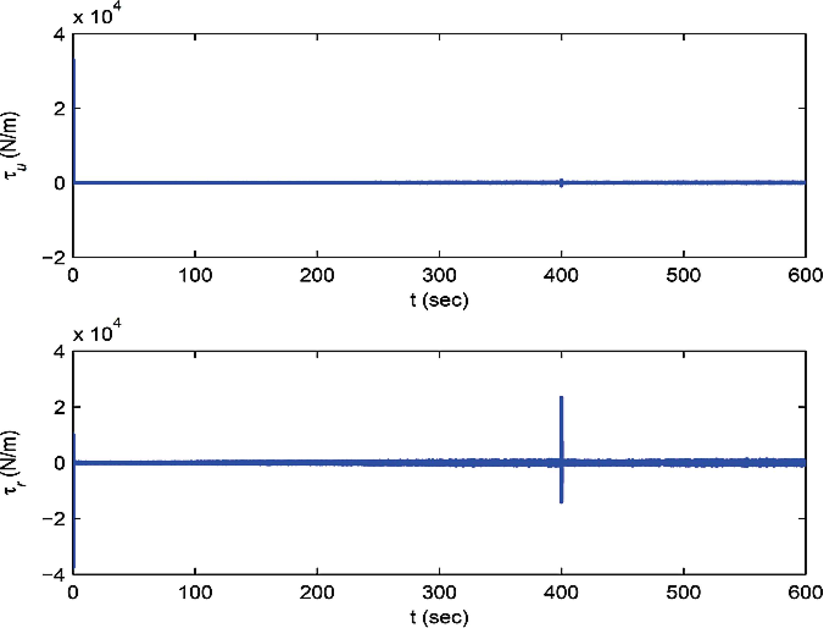
The weights of RBFNN and the adaptive gain are initialized at zero. Figure 1 to Figure 5 illustrate the results of employing the proposed controller (9-a) for the ASV. The movement of ASV in the plane and its heading tracking curve together with estimated states are shown in Figure 1. Figure 2 demonstrates the applied control forces. Observation errors are shown in Figure 3 to Figure 5. It is seen from Figure 1 and Figure 3 that the ASV has realized the tracking task. Figure 4 to Figure 5 illustrate good performance of the designed observer (16) for estimating the unmeasured states. The simulation results imply the effectiveness of the proposed method for control of highly nonlinear systems with unknown dynamics and unmeasured states and its robustness against estimation error, environment disturbances and measurement noises.

Example 2:

The proposed control method in this study is compared with that of Ref. 40 for an underactuated surface vehicle (USV) whose dynamics is given by⁴⁰

(47)h(η,ν)=[2.436u12.992v0.0564r],M=[1.9560002.4050000.403]

Similar to Ref. 40, the initial condition of the robot is η(0) = ν = 0 and the reference trajectory to be tracked is a straight line trajectory. The design parameters are β = 0.75, ρ = 2, k_w = 0.1, k_α = 0.25, η₁ = 1, η₂ = 0.1. The Parameters of RBFNN are selected same as Example 1. Finally, the column full-rank gain matrix G₁ is chosen as

(48)G1=0.002[100.20.211]

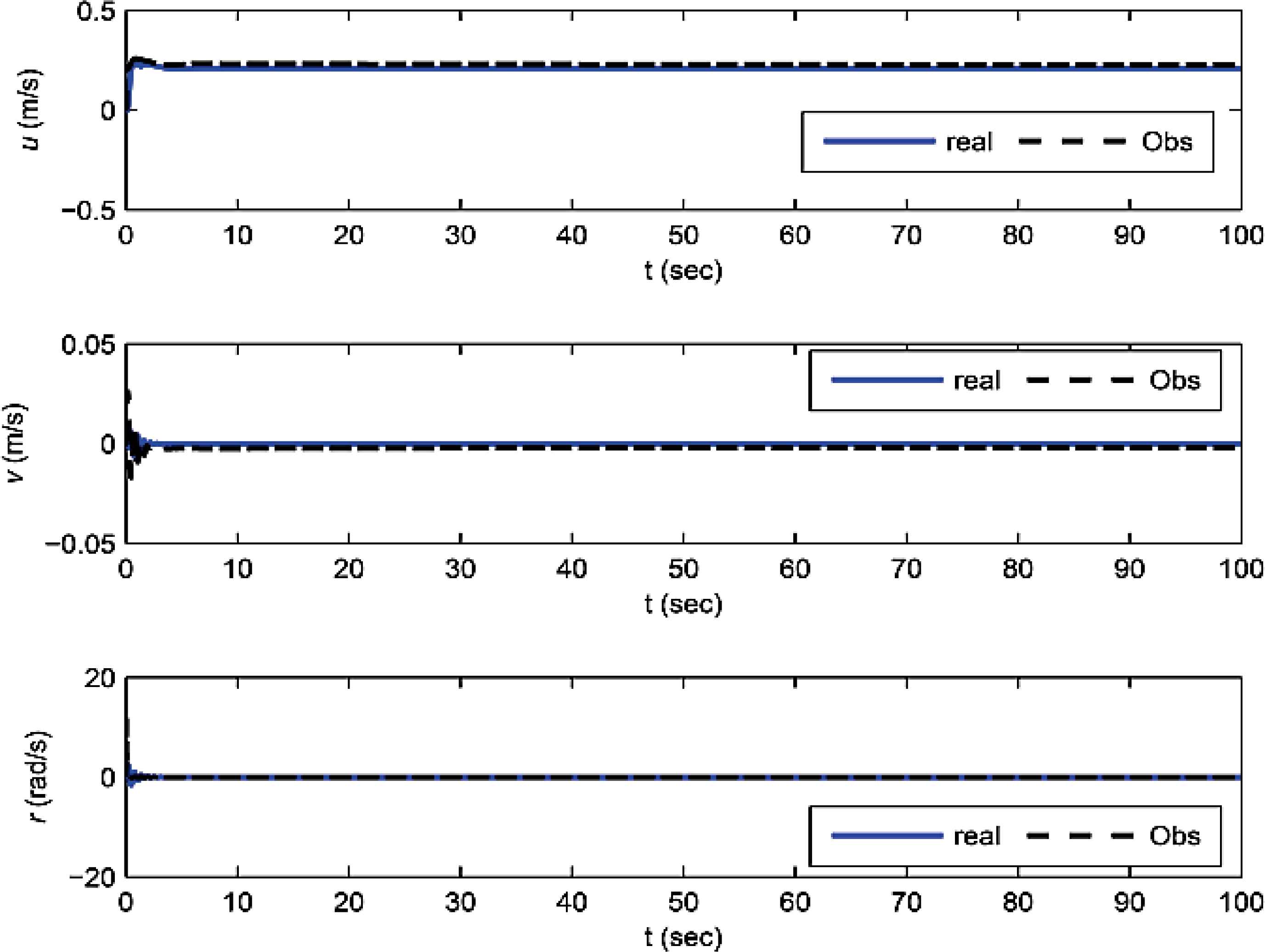
The simulation results are shown in Figure 6 and Figure As shown in Figure 6, the proposed controller can provide faster convergence and higher tracking performance than the controller of Ref. 40. Figure 7 illustrates good performance of the designed observer (16) for estimating the unmeasured states.

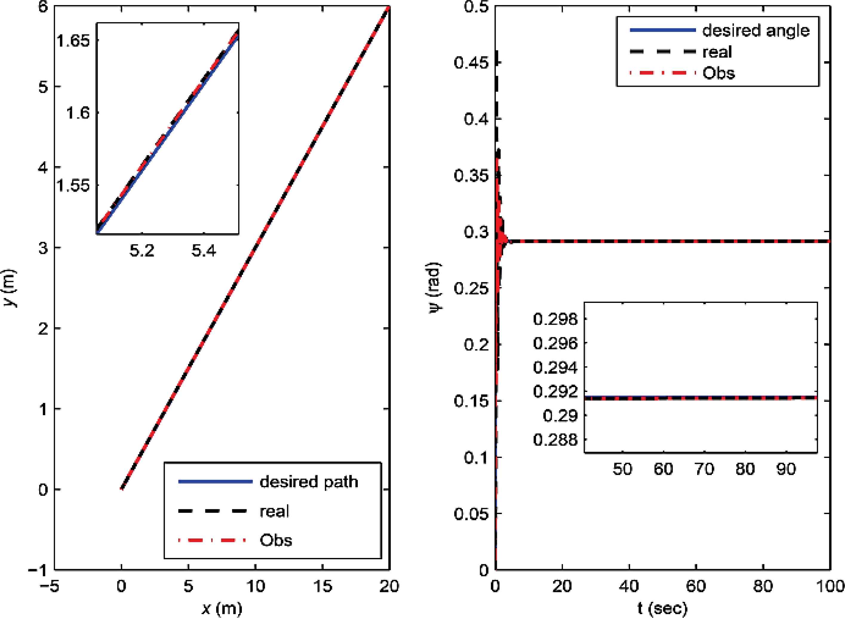
6. Conclusion

This paper has addressed a robust adaptive control based on observer for MIMO non-square nonlinear systems with unknown dynamics. The proposed method is studied for two possible cases, i.e., underactuated and fully-actuated ones. A constant full-rank matrix with an adaptive gain is employed in the control law. Thus, contrast to the majority of the available results which employed two neural networks, the new controller utilizes only one neural network. Furthermore, by filtering the output error, the state variables of the filter are applied to design the underlying update laws. Therefore, the observer does not need to satisfy the SPR conditions. These new contributions result in to simplification of the controller structure and its implementation in practical applications. The Lyapunov analysis is applied to guarantee the closed-loop system stability and convergence of unknown parameters. The simulation results confirm the validity of the proposed controller and its robustness against estimation error, environment disturbances and measurement noises.

References

1.T Hayakawa, MM Haddad, JM Bailey, and N Hovakimyan, Passivity-based neural network adaptive output feedback control for nonlinear nonnegative dynamical systems, IEEE Trans. Neural Netw, Vol. 16, No. 2, 2005, pp. 387-398.

2.G Debbache and N Golea, Neural network based adaptive sliding mode control of uncertain nonlinear systems, J. Syst. Eng. Electr, Vol. 23, No. 1, 2012, pp. 119-128.

3.AK Kostarigka and GA Rovithakis, Adaptive neural network output feedback passivation of MIMO uncertain systems, in 16th Mediterranean Conf. Control Autom. (France, Ajaccio, 2008), pp. 297-302.

4.CP Bechlioulis and GA Rovithakis, Prescribed performance adaptive control for multi-input multi-output affine in the control nonlinear systems, IEEE Trans. Autom. Control, Vol. 55, No. 5, 2010, pp. 1220-1226.

5.EB Kosmatopoulos, Universal stabilization using control Lyapunov functions, adaptive derivative feedback, and neural network approximators, IEEE Trans. Syst. Man, and Cybern., Part B: Cybern, Vol. 28, No. 3, 1998, pp. 472-477.

6.XL Xie, ZG Hou, L Cheng, C Ji, M Tan, and H Yu, Adaptive neural network tracking control of robot manipulators with prescribed performance, Proc. the Inst. Mech. Eng., Part I: J. Syst. Control Eng, Vol. 225, No. 6, 2011, pp. 790-797.

7.Z Wang, A Behal, and P Marzocca, Robust adaptive output feedback control design for a multi-input multi-output aero elastic system, Int. J. Aeronaut.l Space Sci, Vol. 12, No. 2, 2011, pp. 179-189.

8.SS Ge and C Wang, Adaptive neural control of uncertain MIMO nonlinear systems, IEEE Trans. Neural Netw, Vol. 15, No. 3, 2004, pp. 674-692.

9.H Xu and PA Ioannou, Robust adaptive control for a class of MIMO nonlinear systems with guaranteed error bounds, IEEE Trans. Autom. Control, Vol. 48, No. 5, 2003, pp. 728-742.

10.C Wang and Y Lin, Robust adaptive neural control for a class of uncertain MIMO nonlinear systems, Int. J. Syst. Sci, Vol. 46, No. 11, 2015, pp. 1934-1943.

11.S Kolavennu, S Palanki, and JC Cockburn, Nonlinear control of nonsquare multivariable systems, Chem. Eng. Sci, Vol. 56, No. 6, 2001, pp. 2103-2110.

12.S Palankia, JC Cockburn, and S Kolavennu, Robust state feedback synthesis for control of non-square multivariable nonlinear systems, J. of Process Control, Vol. 13, No. 7, 2003, pp. 623-631.

13.S Aloui, O Pag`es, A El Hajjaji, A Chaari, and Y Koubaa, Robust Fuzzy tracking control for a class of perturbed Non-square nonlinear systems, in 2010 American Control Conf. (USA, MD., Baltimore, 2010), pp. 4788-4793.

14.S Aloui, O Pag`es, A El Hajjaji, A Chaari, and Y Koubaa, Generalized fuzzy sliding mode control for mimo nonlinear uncertain and perturbed systems, in 18th Mediterranean Conf. Control & Autom. Congr. (Morocco, Marrakech, 2010), pp. 1164-1169.

15.CL Hwang, CC Chiang, and YW Yeh, Adaptive fuzzy hierarchical sliding-mode control for the trajectory tracking of uncertain underactuated nonlinear dynamic systems, IEEE Trans. Fuzzy Syst, Vol. 22, No. 2, 2014, pp. 286-299.

16.F Nafa, S Labiod, and H Chekireb, Direct adaptive fuzzy sliding mode decoupling control for a class of underactuated mechanical systems, Turkish J. Electr. Eng. Comput. Sci, Vol. 21, No. 6, 2013, pp. 1615-1630.

17.S Aloui, O Pag`es, A El Hajjaji, A Chaari, and Y Koubaa, Robust adaptive fuzzy sliding mode control design for a class of MIMO underactuated system, in Preprints of the 18th IFAC World Congr. (Italy, Milano, 2011), pp. 11127-11132.

18.M Kim, Y Kim, and J Jun, Adaptive sliding mode control using slack variables for affine underactuated systems, in 2012 IEEE 51st Annual Conf. Decis. Control (CDC) (2012), pp. 6090-6095.

19.M Chemachema, Output feedback direct adaptive neural network control for uncertain SISO nonlinear systems using a fuzzy estimator of the control error, Neural Netw, Vol. 36, 2012, pp. 25-34.

20.A Boulkrounea and M M’saad, On the design of observer-based fuzzy adaptive controller for nonlinear systems with unknown control gain sign, Fuzzy Sets Syst, Vol. 201, 2012, pp. 71-85.

21.Y Wang, T Chai, and Y Zhang, State observer-based adaptive fuzzy output-feedback control for a class of uncertain nonlinear systems, Inf. Sci, Vol. 180, No. 24, 2010, pp. 5029-5040.

22.A Boulkrounea, M Tadjineb, and M M’saad, How to design a fuzzy adaptive controller based on observers for uncertain affine nonlinear systems, Fuzzy Sets Syst, Vol. 159, No. 8, 2008, pp. 926-948.

23.HL Choi and JT Lim, Global exponential stabilization of a class of nonlinear systems by output feedback, IEEE Trans. Autom. Control, Vol. 50, No. 2, 2005, pp. 255-257.

24.SS Ge, CC Hang, and T Zhang, Adaptive neural network control of nonlinear systems by state and output feedback, IEEE Trans. Syst. Man Cybernetics, Part B: Cyber, Vol. 29, No. 6, 1999, pp. 818-828.

25.LB Freidovicha and HK Khalil, Lyapunov-based switching control of nonlinear systems using high-gain observers, Automatica, Vol. 43, No. 1, 2007, pp. 150-157.

26.S Frikha, M Djemel, and N Derbel, Observer based adaptive neuro-sliding mode control for MIMO nonlinear systems, Int. J. Control Autom. Syst, Vol. 8, No. 2, 2010, pp. 257-265.

27.YJ Liu, SC Tonga, and TS Li, Observer-based adaptive fuzzy tracking control for a class of uncertain nonlinear MIMO systems, Fuzzy Sets Syst, Vol. 164, No. 1, 2011, pp. 25-44.

28.KS Shih, THS Li, and SH Tsai, Observer-based adaptive fuzzy robust controller with self-adjusted membership functions for a class of uncertain MIMO nonlinear systems: a pso-sa method, Int. J. Innov. Comput. Inf. Control, Vol. 8, No. 2, 2012, pp. 1419-1437.

29.Z Du and Z Qu, Improved adaptive fuzzy control for MIMO nonlinear time-delay systems, J. Control Theory Appl, Vol. 9, No. 2, 2011, pp. 278-282.

30.Y Cheng, W Xie, and W Sun, High gain disturbance observer-based control for nonlinear affine systems, Int. J. Adv. Robot. Syst, Vol. 9, No. 16, 2012.

31.CC Chiang and CH Wu, Observer-based adaptive fuzzy sliding mode control of uncertain multiple-input multiple-output nonlinear systems, in IEEE Int. Fuzzy Syst. Conf. (2007), pp. 1-6.

32.H Saberi Najafi and M Shams Solary, Computational algorithms for computing the inverse of a square matrix, quasi-inverse of a non-square matrix and block matrices, Applied Math. Comput, Vol. 183, No. 1, 2006, pp. 539-550.

33.LX Wang and JM Mendel, Fuzzy basis function, universal approximation, and orthogonal least-squares learning, IEEE Trans. Neural Netw, Vol. 3, No. 5, 1992, pp. 807-814.

34.CY Lee and JJ Lee, Adaptive control for uncertain nonlinear systems based on multiple neural networks, IEEE Trans. Syst. Man, and Cybern., Part B: Cybern, Vol. 34, No. 1, 2004, pp. 325-333.

35.B Karimi and MB Menhaj, Non-affine nonlinear adaptive control of decentralized large-scale systems using neural networks, Inf. Sci, Vol. 180, No. 17, 2010, pp. 3335-3347.

36.E Zergeroglu, W Dixon, D Haste, and D Dawson, A composite adaptive output feedback tracking controller for robotic manipulators, Robotica, Vol. 17, No. 6, 1999, pp. 591-600.

37.JH Parka, GT Parkb, SH Kima, and CJ Moon, Output-feedback control of uncertain nonlinear systems using a self-structuring adaptive fuzzy observer, Fuzzy Sets Syst, Vol. 151, No. 1, 2005, pp. 21-42.

38.H Khalil, Nonlinear Systems, 3rd edn, Prentice Hall, Upper Saddle River, NJ, 2002.

39.M Rayhanoglu, Exponential stabilization of an underactuated autonomous surface vessel, Automatica, Vol. 33, No. 12, 1997, pp. 2249-2254.

40.G Xia, G Wang, X Chen, A Zhao, and C Pang, DRFNN adaptive observer based sliding mode tracking control of an underactuated surface vehicle, in 2015 IEEE Int. Conf. Mech. and Autom. (ICMA) (2015), pp. 2255-2260.

<Previous Article In Issue

Download article (PDF)

Next Article In Issue>

Journal: International Journal of Computational Intelligence Systems
Volume-Issue: 10 - 1
Pages: 23 - 33
Publication Date: 2017/01/01
ISSN (Online): 1875-6883
ISSN (Print): 1875-6891
DOI: 10.2991/ijcis.2017.10.1.3 How to use a DOI?
Open Access: This is an open access article under the CC BY-NC license (http://creativecommons.org/licences/by-nc/4.0/).

Cite this article

ris enw bib

TY  - JOUR
AU  - Hassan Ghiti Sarand
AU  - Bahram Karimi
PY  - 2017
DA  - 2017/01/01
TI  - Observer based robust neuro-adaptive control of non-square MIMO nonlinear systems with unknown dynamics
JO  - International Journal of Computational Intelligence Systems
SP  - 23
EP  - 33
VL  - 10
IS  - 1
SN  - 1875-6883
UR  - https://doi.org/10.2991/ijcis.2017.10.1.3
DO  - 10.2991/ijcis.2017.10.1.3
ID  - Sarand2017
ER  -

download .riscopy to clipboard