
Classification of the risk in the new financing framework of the Deposit Guarantee Systems in Europe: K-Means Cluster Analysis and Soft Computing
- DOI
- 10.2991/ijcis.2017.10.1.6How to use a DOI?
- Keywords
- Deposit Guarantee Systems; European banking system; banking regulation; risk classification; K-means; soft computing
- Abstract
The guidelines published by the European Banking Authority in 2015 about the contributions to the Deposit Guarantee Systems, establish two approaches to classify the member entities’ risk: the bucket method and the sliding scale method, allowing freedom to every Member State to decide which methodology to use. In this work, using the bucket method with two different clustering techniques, k-means and soft computing, in a sample that represents more than 90% of the deposits covered in the Spanish banking system during the 2008 to 2014 period, the differences in the distribution of the Deposit Guarantee Fund risk and in the entities’ contributions is analyzed. The obtained results reveal important differences. Consequently, the technique chosen by each country will determine the contributions regime.
- Copyright
- © 2017, the Authors. Published by Atlantis Press.
- Open Access
- This is an open access article under the CC BY-NC license (http://creativecommons.org/licences/by-nc/4.0/).
1. Introduction
Among the key aspects to secure the financial strength and prevent systemic crisis scenarios are, among others, ensure the safety of the depositors in the credit companies and ensure an orderly management of the bank insolvencies, objectives entrusted to the Deposit Guarantee System (DGS).
Due to the financial crisis, a profound change was boosted in the international regulatory standards aimed at building a more robust banking system, and thereby consolidate financial stability. In this sense the Basel III agreement drawn up by the Basel Committee on Banking Supervision aims to strengthen sound banking, establishing a closer relationship between levels of risk and capital entities. Entities operating at a higher risk should have higher own resources to cope with potential losses avoiding the bankruptcy of the entity. Improve risk management is the basis of the changes in financial regulation, penalizing the institutions taking excessive risks.
The greatest efforts were directed at establishing new frameworks for bank resolution that avoided the authorities from subsequently coming to the rescue, with the consequent burden on the public resources. The pillars of this new agreement1 are four:
- (i)
The requirement for a greater absorption of losses.
- (ii)
The existence of effective resolution regimes.
- (iii)
A reinforced supervisory intensity.
- (iv)
Greater resistance of the market infrastructure.
In Europe, these Guidelines were recently incorporated through the Bank Recovery and Resolution Directive (BRRD)2 that establishes the rules for the resolution of banks and large investment firms and the Directive on the Deposit Guarantee Systems (DDGS)3. Both rules establish that the Member States (EM) will require funds to establish ex contributions paid by banks.
The DDGS establishes, in its Article 13 (3), the commission to the European Banking Authority (EBA) to issue the guidelines specifying the methods for calculating the contributions to the Deposit Guarantee Systems (DGS) and, in particular, will have to include a calculation formula, the specific indicators, the kinds of risks for the members, the risk weights thresholds assigned to specific risk types and other necessary elements. These guidelines are based on the principles agreed upon at an international level, such as the BIS-IADI Basic Principles for Effective Deposit Insurance Systems4 and the IADI General Guidance for the development of differential premiums5.
On May 28th 2015, the EBA publishes the final Guidelines6 “About the methods of calculating the contributions to the Deposit Guarantee System”, and specify five risk categories in order to ensure that a sufficiently wide range of the fundamental aspects in the activity of the entities are reflected in the risk classification: capital adequacy, liquidity and asset quality, business and management model and potential losses for the DGS.
The proposed methods are two, the Bucket Method and the Sliding Scale Method, the EBA allowing the Member Entities freedom to decide which method to use. However, this decision may lead to differences in the contributions by the entities depending on the country, and pose an impediment to the planned harmonization of the future common Guarantee Fund in the European Union.
This work shows how the application of different classification methodologies for a given DGS reflects different risk exposure distributions and consequently an uneven impact on the contributions to be made by the Member Entities. To do this, using the Bucket Method and two different methodologies to classify risk, Cluster analysis7,8 and Clustering techniques based on Soft Computing9,10, analyzes the differences in the risk distribution of the Deposit Guarantee Fund of Credit Institutions in Spain (FGDEC) and the impact on the Member Entities’ contributions from 2008-2014.
The document is structured as follows. The following section presents a review of the related literature. Section 3 analyzes the relevant aspects of the new contributions regime. Section 4 presents the results. Finally, section 5 concludes the document.
2. Background
Internationally there is a consensus on the convenience of establishing financing systems based on risk measures to improve the deposit insurances’ effectiveness. A system with these characteristics will allow defining fairer contributions based on the risk of every insured entity, contributing to a greater market discipline. Charging the banks a flat fee for the deposit insurance, often as a percentage of the deposits, has two major drawbacks. First, it encourages the bank’s risk-taking to maximize the benefits and second, it implies that the lower-risk banks are subsidizing the higher-risk ones11.
The literature proposes three possible approaches for calculating the contributions based on the risk profiles of the DGS members:
- (i)
Using a single indicators’ model.
- (ii)
A multiple indicators’ model.
- (iii)
A default risk model.
The first two models are based on accounting indicators to evaluate the risk profile of the DGS members. Indicators that cover commonly used key areas to evaluate the financial soundness of a bank, such as capital adequacy, liquidity, profitability and asset quality. While the first approach (single indicator model) uses a single indicator based on the accountancy of these categories (for example, the capital adaptation index under the Basel rules) to calculate the risk-based contributions, different studies in the academic field confirm the appropriateness of using the capital ratio or some of the methods established in Basel II to measure risk in order to establish an objective and consistent system of variable premiums12,13,14. The multiple indicator model adds information of different variables to obtain the adjustment coefficient. Currently, the Federal Deposit Insurance Corporation (FDIC) in U.S.A. uses a multiple indicator model based on the CAMELa qualification system.
The credit risk models can be applied if the DGS are considered as holding creditors’ portfolios represented by the banks. Therefore, the use of the option valuation theory originally proposed by Black and Scholes (1973)15 and Merton (1973)16, is possible to fix the price of the deposit insurance cost (Merton, 1977)17. Merton (1977) shows that a DGS can be seen as a sales option on the value of the Bank’s assets with an exercise price equal to the value of its debt maturity. Many of the empirical studies generated by the Merton model focus on the issue of the over or underestimation of the deposit insurance18,19,20,21,22,23. For many banks, the most important drawback of these models is the lack of information on the market prices, which makes the model difficult to apply in practice.
The EBA (2015) states that the DGS must comply with the following principles in developing their calculation methods:
- (i)
the contribution of each member institution must reflect the probability of default of the bank, as well as the potential losses arising from an intervention by the DGS
- (ii)
the contributions must be distributed as evenly as possible over time until the target level is reached, but with due consideration of the phase of the economic cycle and the procyclical impact that the contributions may have on the financial situation of the member banks;
- (iii)
in order to mitigate the moral risk, the incentives provided by the DGS must be compatible with the prudential requirements (i.e., the capital and liquidity requirements reflecting the risk of the member institution);
- (iv)
the calculation methods must take into account the banking sector’s specific characteristics, and be compatible with the regulatory regime, the accounting practices and presentation of reports in the Member State in which the DGS is established;
- (v)
the rules for calculating the contributions must be objective and transparent;
- (vi)
the data necessary for calculating the contributions must not lead to excessive additional information requirements;
- (vii)
the confidential information must be protected; and finally,
- (viii)
the calculation methods must be consistent with the relevant historical data.
The annual contribution to a DGS by a credit entity must be calculated in the following way (EBA, 2015) by Eq. (1):
The contribution rate (CR) is the percentage that a member entity should pay with a global risk weight (ARW) equal to 100% (i.e., assuming there is no risk differentiation in the contributions), in order to meet the annual target level. The DGS will annually establish the contribution rate by dividing the annual target levelb by the amount of the covered deposits of all the member entities.
The global risk weight for a member entity i (ARWi) will be determined according to the added risk score obtained by the entity (ARSi). The ARSi is equal to the sum of the risk weight scores of the different indicators. Two methods are proposed to calculate the ARSi and the assignment of the ARWi: Bucket Method and Sliding Scale Method. In the first, the classification of the risk follows a discrete scale (i.e., using buckets or classes). In the Sliding Scale Method, the classification of the risk follows a continuous scale (it does not require to differentiate buckets or classes).
Finally, the DGS must take into account the phase of the economic cycle and the procyclical impact that the contributions may have on the financial situation of the member institutions when they establish the annual target level. The cyclical adjustment must be made to avoid raising excessive contributions during the economic crises and to allow a more rapid accumulation of the DGS fund in times of economic prosperity.
In a banking system with relatively high-risk institutions, the sum of total annual contributions could be higher that the annual target level that year. Similarly, in a low risk banking system, the sum of total annual contributions would be lower than the annual target level. The adjustment coefficient tries to prevent this discrepancy. It should take into account the risk analysis undertaken by the relevant designated macroprudential authorities and reflect current economic conditions as well as medium-term perspectives, as persistent economic difficulties may not justify low contributions indefinitely. It may also consider the expected evolution in the covered deposits base.
3. Risk Classification Methodology
In this section, the sample considered for the study is described, and then the risk indicators that are selected. Finally, the two risk classifications are presented.
3.1 Sample
The sample considered for the study is made up of 363 credit entities adhered to the Deposit Guarantee Fund of Credit Institutions (FGDEC) from 2008-2014; with a representatively of over 90% of the covered deposits (Table 1). The information used comes from public documents of the Member Entities (annual accounts, reports and information of prudential relevance) and reports of the Deposit Guarantee Fund of Credit Institutions (FGDEC). We use consolidated information, because for some risk indicators is not available at the individual levelc.
| 2008 | 2009 | 2010 | 2011 | 2012 | 2013 | 2014 | |
|---|---|---|---|---|---|---|---|
| Total covered deposits in Spain (millions of Euros) | 736.3 | 781.1 | 790.3 | 792.3 | 794.8 | 796.9 | 788.3 |
| Total covered deposits in the sample (millions of euros) | 651.7 | 730.7 | 686.9 | 790.1 | 781.7 | 791.8 | 781.5 |
| Representativeness of the sample | 88.5% | 93.5% | 86.9% | 99.7% | 98.3% | 99.4% | 99.1% |
| Number of banks | 53 | 69 | 47 | 56 | 49 | 45 | 44 |
Representativeness of the sample
3.2 Selecting the Risk Indicators
To evaluate the different risk categories (capital, liquidity, asset quality, business and management model and potential losses for the DGS), we consider the basic indicators proposed by the EBA (2015: 20) given in Table 2. The information about the liquidity indicators is not available for the study period; proxies have been used from the accounting information available following the recommendations of the EBAd: LCR (Loans / Deposits), NSFR (Stable Financing / Stable Assets), and Liquidity Ratio (Liquid Assets / Total Assets). Table 3 shows some descriptive statistics of the sample in the analyzed period.
| Category | Indicator | Description | Expected sign on bank risk |
|---|---|---|---|
| Capital | Leverage ratio | Tier 1 capital/Total assets | Negative |
| Capital coverage ratio | Actual common equity Tier 1 (CET1) ratio/Required CET1 ratio or, Actual own funds/Required own funds | Negative | |
| CET1 ratio | CET1 capital/Risk weighted assets (RWA) | Negative | |
| Liquidity and Funding | Liquidity coverage ratio (LCR) | LCR ratio as defined in Regulation (EU) No 575/2013 once it becomes fully operational. | Negative |
| Net stable funding ratio (NSFR) | NSFR ratio as defined in Regulation (EU) No 575/2013 once it becomes fully operational. | Negative | |
| Liquidity ratio | Liquid assets/Total assets | Negative | |
| Asset quality | Non-performing loans (NPL) ratio | NPL/Total loans and debt instruments | Positive |
| Business model and management | RWA/TA ratio | RWA/Total assets | Positive |
| Return on assets (ROA) | Net Income/Total assets | Positive/Negative | |
| Potential losses for the DGS | Unencumbered assets/covered deposits | (Total assets – Encumbered assets)/Covered deposits | Positive |
Source: EBA (2015)
Core risk indicators proposed by the EBA (2015)
| Leverage (%) | Capital coverage (%) | CET1 (%) | LTD (%) | SF/SA (%) | Liquidity (%) | NPL (%) | RWA/TA (%) | ROA (%) | UE/CD (%) | |
|---|---|---|---|---|---|---|---|---|---|---|
| Average | 6.80 | 178.44 | 12.34 | 92.44 | 149.67 | 25.78 | 5.62 | 58.69 | 0.07 | 406.89 |
| Median | 5.95 | 158.35 | 10.63 | 92.04 | 113.73 | 19.23 | 4.42 | 60.06 | 0.32 | 303.27 |
| Standard Deviation | 5.62 | 95.57 | 8.01 | 41.02 | 135.41 | 20.98 | 4.01 | 29.96 | 2.25 | 424.34 |
| Minimum | 0.47 | 54.47 | 1.11 | 2.27 | 43.42 | 1.89 | 0.04 | 9.10 | −15.24 | 189.99 |
| Maximum | 72.96 | 811.12 | 62.99 | 311.21 | 1117.29 | 95.87 | 23.00 | 441.94 | 12.03 | 1,197.5 |
| Number of observations | 363 | 363 | 363 | 363 | 363 | 363 | 363 | 363 | 363 | 363 |
Note: Leverage is the leverage ratio (Tier 1 capital/total assets), Capital coverage is the capital coverage ratio (actual own funds/required own funds), CET1 is the CET1 ratio (CET1 capital/risk weighted assets), LTD is the loans-to-deposits ratio, ST/SA is the stable funding/stable assets ratio, Liquidity is the liquidity ratio (liquid assets/total assets), NPL is the non-performing loans ratio, RWA/TA is the risk weighted assets/total assets ratio, ROA is the return on assets (net income/total assets), UE/CD is the unencumbered assets/covered deposits ratio
Descriptive statistics of risk indicators (2008-2014)
3.3 Risk Classification: Cluster Analysis and Soft Computing Analysis
The choice of the “Bucket Method” to calculate the ARW, involves defining a fixed number of buckets for each risk indicator by setting upper and lower limits for each one. The number of buckets for each risk indicator must be at least two, and reflect the different risk profiles of the member institutions (e.g., high, medium, low risk). An individual risk score (IRS), based on these risk levels, will be assigned to each bucket, ranging from 0 to 100, where 0 indicates the lowest risk and 100 the highest. The limits of the buckets can be determined either relatively or absolutely.
When the relative base is used, the banks’ IRS depends on their risk position in the vis-à-vis relation to other institutions (i.e., banks with similar risk profiles can be assigned to different buckets). However, when the absolute base is used, the limits of the buckets are determined to reflect the degree of risk of a specific indicator, i.e., all of the institutions may end up in the same bucket if they all have the same degree of risk level)e. We consider four buckets in our study, where bucket 1 indicates the lowest risk and bucket 4 the highest risk. As we assume a linear application of the IRS to the buckets, the assigned IRS are 0 (bucket 1), 33 (bucket 2), 66 (bucket 3) and 100 (bucket 4). To establish the limits of the buckets we use two classification methodologies: Cluster Analysis and Soft Computing Analysis.
Cluster analysis is a methodology that is widely used among the unsupervised learning techniques whose aim is data analysis and its interpretation 24. It aims at the separation of a set of data objects in a number of groups called clusters through a similarity measure, such that the data objects classified in the same cluster are more similar than any other data object belonging to another cluster 7. Normally every cluster is represented by a prototype or cluster center that characterizes all the data objects belonging to this cluster. Different clustering algorithms obtain the cluster centers as the centroid of the data that belongs to that cluster. This analysis does not impose a priori restrictions on the structure of the data and does not require assumptions about the probabilistic nature (or independence) of the observations25. Although several strategies have been proposed to determine the clusters26,27, the most common method is the relocation of k-means groups28,29.
In the k-means clustering, the formation begins with an initial division, and by means of successive tests, contrasts the effect the allocation of each of the data has on the residual variance to each group30. The minimum value of the variance determines a configuration of new groups with their respective means. It continues to reallocate the data objects to the new centroids, repeating the process until no transfer can reduce the variance or has reached another established stopping criterion. The analysis configures the groups maximizing, in turn, the distance between the centers of gravity and provides a predetermined number of excluding homogeneous clusters, with the maximum divergence between them. To carry out the k-means clustering of indicators from 2008-14f, the Eq. (2) is used, where dij is the similarity measure between observation i and center j.
In the study, the SPSS programg is used, which implements the algorithm described above with the following parameters:
- •
Number of clusters, j={1,..,4}
- •
Initializing cluster centers = Random
- •
Stop criterion = Maximum number of iterations equal to 10
- •
Similarity measure = Euclidean distance.
The traditional or crisp clustering methods, such as the k-means31, are partition methods in which every data object is assigned to a single cluster. However, this course of action does not always provide a convincing partitioned data representation and that is why; clustering methods based on soft computing techniques such as fuzzy clustering were later proposed32. In the fuzzy clustering methods, each data object may belong to multiple clusters with a membership degree7 between zero and one, the sum of the membership degrees of a data object to each cluster being equal to one. Every data object is associated with a membership degree for each cluster, if the membership degree is close to the value of one; such data object represents a high similarity with the data objects contained in that cluster while a degree close to zero membership implies a low similarity between them.
Fuzzy clustering methods are based on objective functions seeking cluster centers for a predefined number of clusters and assign the data objects a fuzzy membership degree for every cluster in an iterative process that minimizes the objective function9,10. A number of fuzzy clusters can be provided in the fuzzy version that represents the maximum number of fuzzy clusters to which every data object can belong, i.e., 0 being the membership degree of that object to the rest of the clusters. Among the most widely used fuzzy clustering methods is the Fuzzy C-Means33 algorithm that uses an optimization process in which the cluster centers and the data objects are updated to find a local optimum.
To carry out the Fuzzy C-Means clustering of indicators from 2008–14h, the Eq. (3) is used, where uij is the membership of observation i in cluster j, and dij is the similarity measure between observation i and cluster center j.
In this study, the following describes the parameters used to obtain the Fuzzy C-Means clusters for the sample of indicators from 2008-14 that have been carried out by using the R software i:
- •
Number of clusters = 4
- •
Maximum number of fuzzy clusters = 2
- •
Initializing cluster centers = Random
- •
Stop criterion = Maximum number of iterations equal to 10
- •
Similarity measure = Euclidean distance
The limits of the buckets obtained with the different analyzes by indicator are shown in Table 4.
| Risk Indicator (RI) | Analysis | Bucket 1 (IRS = 0) | Bucket 2 (IRS = 33) | Bucket 3 (IRS = 66) | Bucket 4 (IRS = 100) |
|---|---|---|---|---|---|
| Leverage | Cluster | RI > 8% | 8% ≥ RI > 6.1% | 6.1% ≥ RI > 4.5% | RI ≤ 4.5% |
| Soft Computing | RI > 11.7% | 11.7% ≥ RI > 6.8% | 6.8% ≥ RI > 4.4% | RI ≤ 4.4% | |
| Capital coverage | Cluster | RI > 196.1% | 196.1% ≥ RI > 167.1% | 167.1% ≥ RI > 140.5% | RI ≤ 140.5% |
| Soft Computing | RI > 180.6% | 180.6% ≥ RI > 177.9% | 177.9% ≥ RI > 143.7% | RI ≤ 143.7% | |
| CET1 | Cluster | RI > 13.9% | 13.9% ≥ RI > 10.8% | 10.8% ≥ RI > 7.9% | RI ≤ 7.9% |
| Soft Computing | RI > 21.0% | 21.0% ≥ RI > 12.4% | 12,4% ≥ RI > 9.0% | RI ≤ 9.0% | |
| LTD | Cluster | RI < 53.9% | 53.9% ≤ RI < 92.9% | 92.9% ≤ RI < 129.8% | RI ≥ 129.8% |
| Soft Computing | RI < 53.8% | 53.8% ≤ RI < 92.2% | 92.2%≤ RI < 139.0% | RI ≥ 139.0% | |
| SF/SA | Cluster | RI > 201.5% | 201.5% ≥ RI > 132.8% | 132.8% ≥ RI > 90.9% | RI ≤ 90.9% |
| Soft Computing | RI > 422.2% | 422.2% ≥ RI > 270.7% | 270.7% ≥ RI > 114.9% | RI ≤ 114.9% | |
| Liquidity | Cluster | RI > 41.7% | 41.7% ≥ RI > 25.7% | 25.7% ≥ RI > 14.7% | RI ≤ 14.7% |
| Soft Computing | RI > 58.4% | 58.4%≥ RI > 28.3% | 28.3% ≥ RI > 15.3% | RI ≤ 15.3% | |
| NPL | Cluster | RI < 3.7% | 3.7% ≤ RI < 6.7% | 6.7% ≤ RI < 10.4% | RI ≥ 10.4% |
| Soft Computing | RI < 3.4% | 3.4% ≤ RI < 6.5% | 6.5%≤ RI < 10.7% | RI ≥ 10.7% | |
| RWA/TA | Cluster | RI < 35.5% | 35.5% ≤ RI < 56.6% | 56.6% ≤ RI < 71.63% | RI ≥71.63% |
| Soft Computing | RI < 32.0% | 32.0% ≤ RI < 52.2% | 52.2%≤ RI < 66.5% | RI ≥ 66.5% | |
| ROA | Cluster | RI > 0.92% | 0.92% ≥ RI > 0.56% | 0.56% ≥ RI > 0.29% | RI ≤ 0.29% |
| Soft Computing | RI > 1.6% | 1.6%≥ RI >0.4% | 0.4% ≥ RI > -1.6% | RI ≤ -1.6% | |
| UE/CD | Cluster | RI > 433.7% | 433.7% ≥ RI > 340.8% | 340.8% ≥ RI > 277.4% | RI ≤ 277.4% |
| Soft Computing | RI > 970.0% | 970.0%≥ RI > 589,9% | 589,9% ≥ RI > 335.5% | RI ≤ 335.5% | |
Buckets for risk indicators: Analysis Cluster y Analysis Soft Computing
The added risk score (ARS) for i bank is calculated by Eq. (4):
In the case of only using key risk indicators to determine the contributions to the DGS, the EBA (2015) recommends assigning the following weights to the risk categories: capital, 24%; liquidity and financing, 24%; asset quality, 18%; business and management model, 17%; and, finally, the potential use of the DGS funds, 17%.
The specific IW assigned to each risk indicator is presented in Table 5.
| Risk categories and risk indicators | Weights |
|---|---|
| Capital | 24% |
| Leverage | 8% |
| Capital coverage | 8% |
| CET1 | 8% |
| Liquidity and funding | 24% |
| LTD | 8% |
| SF/SA | 8% |
| Liquidity | 8% |
| Asset quality | 18% |
| NPL | 18% |
| Business model and management | 17% |
| RWA/TA | 8.5% |
| ROA | 8.5% |
| Potential losses for the DGS | 17% |
| UE/CD | 17% |
Weights for risk categories and risk indicators
The risk scores (ARS) must be grouped into risk levels, and these have a weight assigned (ARW) to calculate the individual contribution of a bank to the DGS according to the expression [1]. Following the recommendations of the EBA (2015), we consider the following classes and risk weights: low risk, 50%; medium risk, 100%; high risk, 150% and very high risk, 200%. For grouping risk scores and the definition of the risk types’ limits, we once again use cluster analysis and soft computing. The obtained results are shown in Table 6.
| Risk class | ARW | Cluster analysis | Soft Computing analysis |
|---|---|---|---|
| Low | 50% | ARS < 35.08 | ARS < 35.89 |
| Medium | 100% | 35.8 ≤ ARS < 50.66 | 38,89 ≤ ARS < 57,42 |
| High | 150% | 50.66 ≤ ARS < 63.78 | 57,42 ≤ ARS < 69,98 |
| Very high | 200% | ARS ≥ 63.78 | ARS ≥ 69,98 |
Risk classes: Cluster and Soft Computing.
4. Results
The use of both methodologies in the risk classification of the entities evidence appreciable differences in both risk distribution and the consequences of the entities’ contributions to the Deposit Guarantee Fund of Credit Institutions (FGDEC).
From the results presented in Table 7, it is observed that the score for medium risk is higher with the soft computing analysis and a little more than half of the entities, they would have a risk score equal to or greater than 63.20 points, reducing to 54.53 with the cluster analysis. However, the degree of dispersion regarding the average is similar with both techniques.
| ARS | Cluster Analysis | Soft Computing Analysis |
|---|---|---|
| Average | 52.62 | 60.48 |
| Median | 54.53 | 63.20 |
| Standard Deviation | 14.70 | 15.45 |
| Coefficient of variation | 0,28 | 0,26 |
| Asymmetry | −0.605 | −1.050 |
| Kurtosis | 0.193 | 1.274 |
| Minimum | 5.28 | 8.09 |
| Maximum | 86.23 | 97.28 |
| Number of observations | 363 | 363 |
Descriptive statistics of ARS (2008-2014)
Both distributions have negative asymmetry, more pronounced with soft computing analysis. In Figure 1 and 2, we can see a greater accumulation of entities in the right lane with the soft computing classification, which shows a higher level of risk in the Deposit Guarantee Fund of Credit Institutions (FGDEC) with this classification procedure.
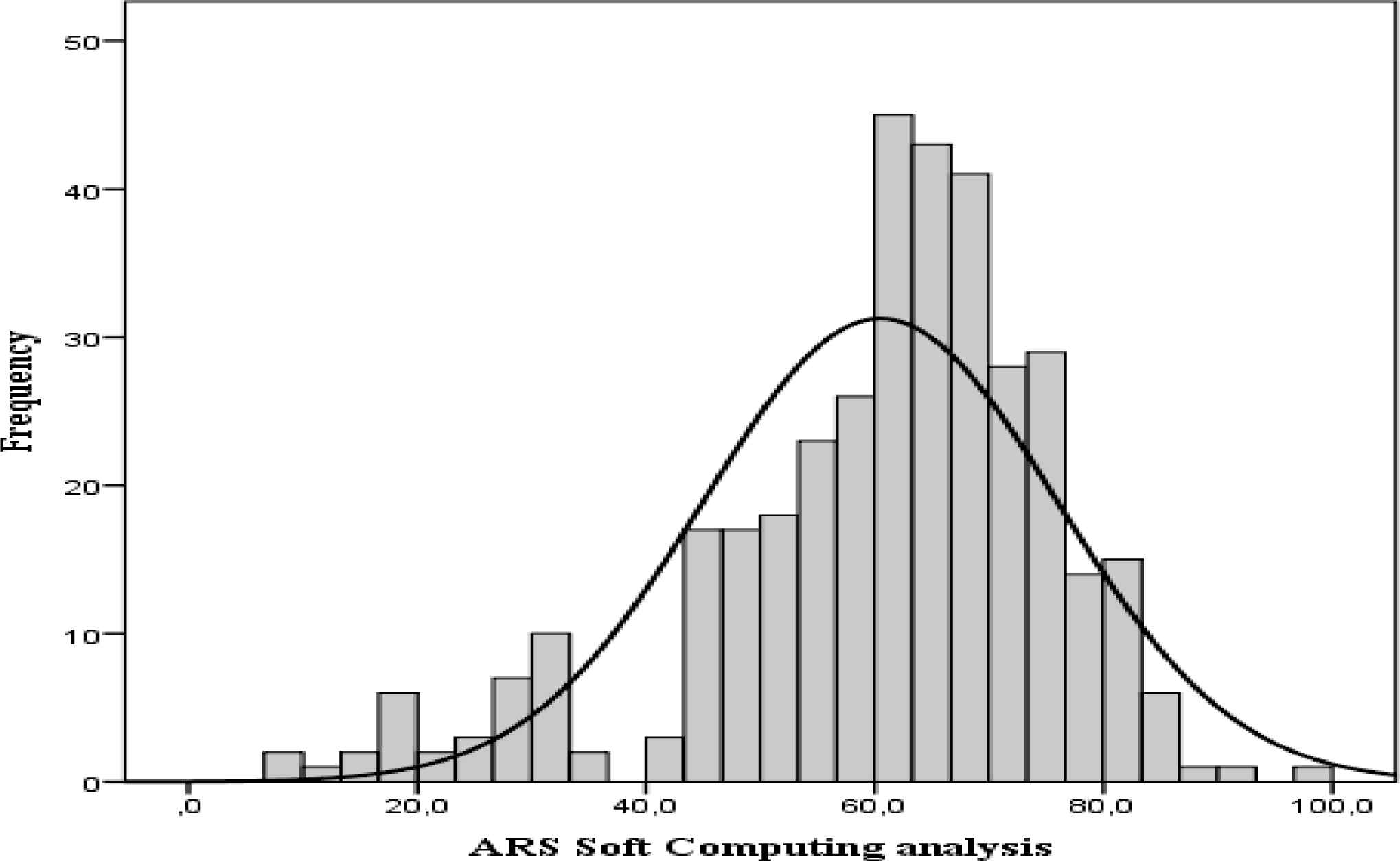
Frequency distribution ARS with Soft computing
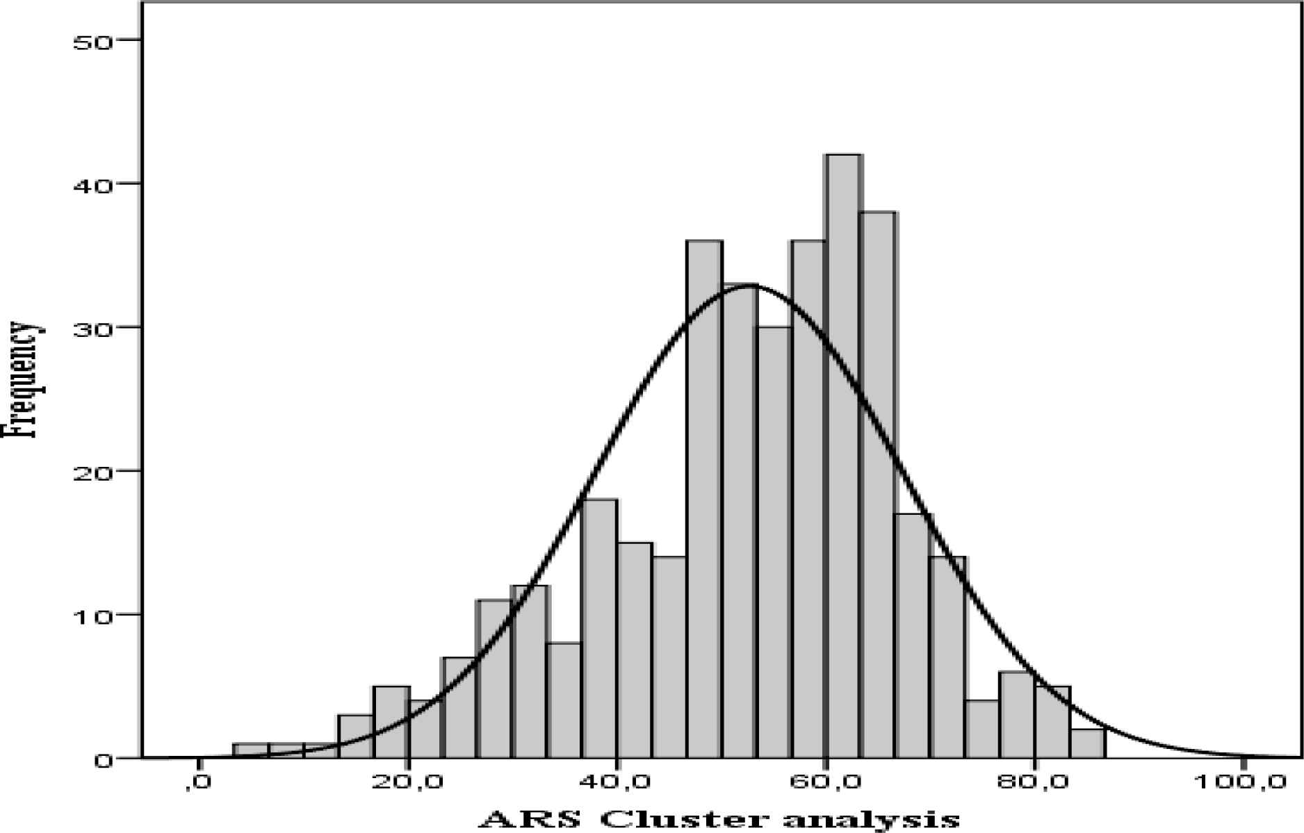
Frequency distribution ARS with Cluster analysis
If we look at the distribution of covered deposits at the risk levels established by both techniques (Figure 3), and taking into account the level of risk associated with the DGS depending on the number of entities in each risk category and, the volume of covered deposits in each one, the distribution of the covered deposits present significant differences according to the classification procedure, mainly in the lanes. The entities classified as of low risk with the cluster analysis account for 13.4% of the Deposit Guarantee Fund of Credit Institutions (FGDEC) deposits, compared to the 0.4% of the soft computing analysis. The higher risk entities group 21.2% of the deposits covered with the soft computing analysis, compared to the 15% of the cluster analysis. Therefore, the distribution of the covered deposits represents a higher risk for the Deposit Guarantee Fund of Credit Institutions (FGDEC) when soft computing is used as a classification technique.

Distribution of deposits covered risk levels (08-14)
To reflect the above results in the total contributions to be undertaken by the entities to the Deposit Guarantee Fund of Credit Institutions (FGDEC), we calculate the risk-adjusted contributions according to the Eq. (1) from the classifications obtained with both analyzes. We determine the contribution rate (CR) needed to achieve the annual patrimony target level and the adjustment coefficient (µ) for every year to avoid the procyclicality of the contributions as established by the EBA (2015), the obtained results are shown in Table 8.
| 2008 | 2009 | 2010 | 2011 | 2012 | 2013 | 2014 | 2008-14 | |
|---|---|---|---|---|---|---|---|---|
| Contribution rate (CR) | 0.080% | 0.081% | 0.080% | 0.084% | 0.084% | 0.085% | 0.083% | 0.082% |
| Total annual risk-unadjusted contributions (millions of Euros) | 521,4 | 591,6 | 547,8 | 664,4 | 655,2 | 672,1 | 651,2 | 614,8 |
| Total annual risk-adjusted contributions (millions of Euros) | ||||||||
| i) Cluster analysis | 604,8 | 628,8 | 678,5 | 860,8 | 906,3 | 847,0 | 819,0 | 763,6 |
| ii) Soft Computing analysis | 655,7 | 772,9 | 699,4 | 932,3 | 959,9 | 977,4 | 870,2 | 838,3 |
| Adjustment coefficient (µ) | ||||||||
| i) Cluster analysis | 0.86 | 0.94 | 0.81 | 0.77 | 0.72 | 0.79 | 0.80 | 0.81 |
| ii) Soft Computing analysis | 0.80 | 0.77 | 0.78 | 0.71 | 0.68 | 0.69 | 0.75 | 0.74 |
Contribution rates and adjustment coefficients
To calculate the CR in the different years covered by the study, we have made the following considerations:
- (i)
In 2008, the FGDEC starts collecting contributions with the aim of achieving the target level of 0.8% of the deposits covered in 10 years (i.e., in 2017);
- (ii)
The contributions are distributed evenly from the initial period; and
- (iii)
Every year the contributions collected by the FGDEC will be equal to the annual target level set for that year.
The total amount of the risk-adjusted contributions confirms the differences already detected in the risk distributions. Applying the soft computing methodology involves greater risk adjusted contributions than with cluster analysis, evidencing an increased risk for the Deposit Guarantee Fund of Credit Institutions (FGDEC). Finally, the amount to be raised cannot exceed the target level set by the Fund, being necessary to use the adjustment coefficient (µ) to determine the final contribution with both methodologies.
Finally, we evaluate the impact of the two classification methodologies on the Member Entities to the Deposit Guarantee Fund of Credit Institutions (FGDEC). To do this, we compare the contributions that each entity would have to make to the Deposit Guarantee Fund of Credit Institutions (FGDEC) to achieve the annual target level without considering the risk with the risk-adjusted contributions, from the relative change between the two contributions:
Where c0 contribution without risk to the planned annual target level, equal to the annual contribution rate for the deposits covered by the entity. ciM risk-adjusted contribution (according to Eq. (1)) in the different methods for risk classification. We analyze the differences between the classification methodologies from the following measures: Percentage of entities that would increase / decrease their contribution, increase / decrease average contributions and variation range (maximum increase and maximum decrease). The obtained results are shown in Table 9.
| Cluster analysis | Soft Computing analysis | |||||||||
|---|---|---|---|---|---|---|---|---|---|---|
| Banks | Mean | SD | Min. | Max. | Banks | Mean | SD | Min. | Max. | |
| Banks that reduce their contribution | 38.3% | -32.8% | 20.7 | -63.9% | -5.9% | 34.4% | -36.4% | 17.4 | -65.9% | -20.5% |
| Banks that increase their contribution | 61.7% | 37.7% | 21.8 | 8.4% | 88.1% | 65.6% | 26.0% | 18.2 | 2.4% | 59.0% |
| Low risk | 13.5% | -59.6% | 3.0 | -63.9% | -53.0% | 9.6% | -63.5% | 2.0 | -65.9% | -60.2% |
| Medium risk | 24.8% | -18.2% | 7.2 | -27.7% | -5.9% | 24.8% | -25.8% | 4.1 | -31.7% | -20.5% |
| High risk | 40.5% | 24.4% | 11.2 | 8.4% | 41.1% | 39.4% | 12.3% | 6.2 | 2.4% | 19.3% |
| Very high risk | 21.2% | 63.1% | 12.4 | 44.6% | 88.1% | 26.2% | 46.6% | 8.1 | 36.5% | 59.0% |
Effect of risk-adjusted contributions: Cluster analysis and Soft Computing analysis (2008-2014)
We found that during the periodunder review, most of the Member Entities would increase their contribution with the new risk-adjusted financing system (around 62% with the cluster analysis and 66% with the soft computing analysis). In the cluster analysis the average increase in contributions would be higher (37.7%) than in the soft computing analysis (26%), it would also produce greater variations between the entities that increase their contribution. For high risk institutions, the average contribution would rise to 5.2 million Euros with the cluster analysis and 4.3 million Euros with Soft Computing analysis. On the contrary, for the entities that reduce contribution, the average decrease would be greater with the soft computing analysis (36.4%) than in the cluster analysis (32.8%). For low risk institutions the contributions decreased in 6 million Euros with Soft Computing analysis and 4.6 million with cluster analysis. The entities classified within the highest risk levels would have a greater penalty (would contribute more) with the cluster classification. While the entities that best manage their risk would benefit from greater reductions in their contributions to the soft computing classification.
5. Conclusions
Among the key aspects to strengthen financial stability and prevent systemic crisis scenarios are, among others, ensure the safety of the depositors in the credit entities and ensure an orderly management of the bank insolvencies, objectives entrusted to the DGS. The last major financial crisis showed that the DGS suffered from significant limitations, leading the European and international authorities to establish measures to improve their funding system while favoring the credit entities’ market discipline. In this context the EBA, at the request of the European Commission, published the Guidelines on the methods of calculating the contributions to the Deposit Guarantee System adjusted to the risk of each entity with the aim of harmonizing the methods to establish contributions in all the Member Entities of the European Union and facilitate the future creation of the Single European Fund in 2015.
However, although the EBA proposes two calculation methods (Bucket Method and Sliding Scale Method) to determine the contributions of the entities to the DGS, instead it allows every country the discretion to decide on the methodology used to determine the risk of every entity and carry out, according to the reached level, the contributions to the system. This competence attributed to every Member Entity can assume significant differences when it comes to quantifying the risk of the DGS and consequently disparity in the contributions depending on every entity’s country of origin.
This work, using the Bucket Method proposed by the EBA, applies two different methodologies to classify the risk for one and the same Deposit Guarantee System (Deposit Guarantee Fund of Credit Institutions), cluster analysis and soft computing analysis, and evidences the situation described above, the risk exposure distributions are different depending on the technique used and therefore a different effect on the contributions that the member entities would have to carry out. Several conclusions can be drawn from the analysis carried out for the regulator, although, the most relevant is the uneven impact when it comes to classifying the risk of every entity depending on the technique used and therefore the contributions to make according to the country where the entity is, having reason to believe that this arbitrariness is an important obstacle in the planned unification of the DGS in the EU.
It would be interesting to extend the effect of the proposal to the different DGS in the EU to determine the impact of the different classification methodologies in the risk profile of DGS of each country, especially when in the future it could be convenient to determine capital requirements of the DGS in line with Basel III recommendations for financial institutions.
Footnotes
CAMEL is an acronym for the following five components of bank safety and soundness: capital sufficiency, asset quality, management quality, earnings and liquidity capability.
The annual target level must be established, at least, by dividing the amount of financing means the DGS needs to raise in a given year in order to reach the target level, for the remaining period of accumulation (expressed in years) to achieve the target level.
The values of the risk indicators must be calculated on an individual basis for each member entity. However, the value of the risk indicators must be calculated on a consolidated basis when the Member State makes use of the option provided for in Article 13 (1) of the Directive 2014/49/UE to allow the central body and all the credit institutions permanently affiliated to the central organism referred to in Article 10 (1) of the Regulation (UE) 575/2013, to be subject as a whole for the risk weighting determined for the central organism and its affiliated entities on a consolidated basis. When a member entity has received an exemption from the compliance with the capital and / or liquidity requirements on an individual basis in accordance with Articles 7, 8 and 21 of the Regulation (UE) 575/2013, the corresponding capital / liquidity indicators must be calculated at a consolidated or semi-consolidated level.
Within each category, the calculation method must include the basic risk indicators specified in Table 2. Exceptionally, any of these indicators may be excluded when it is not available. In this case, the competent authorities must strive to use a proxy as appropriate as possible for the removed indicator (EBA, 2015:20).
However, the EBA (2015) states that the limits of certain buckets over the absolute base must ensure that there is enough and significant differentiation of the member institutions for each risk indicator.
Before carrying out the cluster analysis we eliminate the extreme values of the sample, which could distort the formation of clusters. However, these observations are classified according to the limits established by the cluster analysis.
http://www-01.ibm.com/software/es/analytics/spss/
Before carrying out the cluster analysis we eliminate the extreme values of the sample, which could distort the formation of clusters. However, these observations are classified according to the limits established by the cluster analysis.
References
Cite this article
TY  - JOUR
AU  - Pilar Gómez
AU  - Antonio Partal
AU  - Macarena Espinilla
PY  - 2017
DA  - 2017/01/01
TI  - Classification of the risk in the new financing framework of the Deposit Guarantee Systems in Europe: K-Means Cluster Analysis and Soft Computing
JO  - International Journal of Computational Intelligence Systems
SP  - 78
EP  - 89
VL  - 10
IS  - 1
SN  - 1875-6883
UR  - https://doi.org/10.2991/ijcis.2017.10.1.6
DO  - 10.2991/ijcis.2017.10.1.6
ID  - Gómez2017
ER  -