
Computer Aided Diagnosis System-A Decision Support System for Clinical Diagnosis of Brain Tumours
Current Address: Department of Robotics, Control and Image, cole Centrale de Nantes, 44000, France.
- DOI
- 10.2991/ijcis.2017.10.1.8How to use a DOI?
- Keywords
- Computer aided diagnosis (CAD); Region of interest(s) (ROIs); Magnetic resonance (MR); Artificial neural network (ANN); Graphical user interface (GUI)
- Abstract
The iso, hypo or hyper intensity, similarity of shape, size and location complicates the identification of brain tumors. Therefore, an adequate Computer Aided Diagnosis (CAD) system is designed for classification of brain tumor for assisting inexperience radiologists in diagnosis process. A multifarious database of real post contrast T1-weighted MR images from 10 patients has been taken. This database consists of primary brain tumors namely Meningioma (MENI- class 1), Astrocytoma (AST- class 2), and Normal brain regions (NORM- class 3). The region of interest(s) (ROIs) of size 20 x 20 is extracted by the radiologists from each image in the database. A total of 371 texture and intensity features are extracted from these ROI(s). An Artificial Neural Network (ANN) is used to classify these three classes as it shows better classification results on multivariate non-linear, complicated, rule based domains, and decision making domains. It is being observed that ANN provides much accurate results in terms of individual classification accuracy and overall classification accuracy. The four discrete experiments have been performed. Initially, the experiment was performed by extracting 263 features and an overall classification accuracy 78.10% is achieved, however, it was noticed that MENI (class-1) was highly misclassified with AST (class-2). Further, to improve the overall classification accuracy and individual classification accuracy specifically for MENI (class-1), LAWs textural energy measures (LTEM) are added in the feature bank (263+108=371). An individual class accuracy of 91.40% is obtained for MENI (class-1), 91.43% for AST (class-2), 94.29% for NORM (class-3) and an overall classification accuracy of 92.43% is achieved. The results are calculated with and without addition of LTEM feature with Principle component analysis (PCA)-ANN. LTEM-PCA-ANN approach improved results with an overall accuracy of 93.34%. The texture patterns obtained were clear enough to differentiate between MENI (class-1) and AST (class-2) despite of necrotic and cystic component and location and size of tumor. LTEM detected fundamental texture properties such as level, edge, spot, wave and ripple in both horizontal and vertical directions which boosted the texture energy.
- Copyright
- © 2017, the Authors. Published by Atlantis Press.
- Open Access
- This is an open access article under the CC BY-NC license (http://creativecommons.org/licences/by-nc/4.0/).
1. Introduction
One of the prominent reasons of deaths worldwide is due to brain tumors. Brain tumors are of two type viz. benign and malignant. Benign brain tumors are very slow growing in nature while malignant brain tumors are fast growing in nature and after some time, they may turn into secondary brain tumors. Brain tumors are generally categorized in primary brain tumors and secondary brain tumors. Primary brain tumors are further categorized into many classes such as Glioma, Meningioma, Astrocytoma, Oligodendrogliomas etc. According to World Health Organization (WHO) more than 120 classes are given. The origin of primary brain tumors is in the brain itself while secondary brain tumors originate in any other part of the body and travel towards the brain as Metastatic (METS) tumor. These brain tumors are analyzed and visualized with the help of Magnetic Resonance Imaging (MRI). The detailed images of any part of body are obtained with the help of radio-waves and magnetic field provided through the MRI machine.
These detailed images differ from tumor to tumor, and relaxation time of the excited atoms. These MR images have different texture and intensity patterns for different brain tumors. The texture and intensity of these brain tumors is categorized as isointense, hypo intense or hyper intense. The normal brain cells and tumorous brain cells having similar signal intensity is called iso-intense while tumorous brain cells having darker signal intensity than normal brain cells, is called hypo-intense. If tumorous brain cells have brighter intensity than normal brain cells then it is called hyper-intense.
The person affected from brain tumor may be relieved from mental pressure and pain by timely and proper diagnosis. The brain tumor classification is always an intricate task for radiologists. The reason being iso-intense to hypo-intense properties of brain tumors and inexperience. It is also a hideous task due to the large variance in tumor cells and its infiltration into the adjacent healthy cells. The complexity for classifying brain tumors further depends on its shape, location, size and its intensity and texture of tumorous cells with neighboring normal cells. Though many alternatives such as medication and surgery in the field of medical science have already been developed. However, further assistance is always a requirement for easing up the radiologists in the diagnosis process. A similar initiative is being presented in this paper by developing a CAD system to classify brain tumors on post contrast T1 MR-images. These images are obtained by introducing gadolinium material which enhances contrast. Typically, 0.15-0.20 mMol/kg gadolinium is introduced in patients for contrast enhancement. This results a considerable contrast difference between fluid and solid anatomical structures within the body. Post-contrast T1-weighted MR images are taken as a database for better and large feature bank extraction based on intensity and texture discrimination. In conventional echo repetition time (TR) (<750ms) and echo time (TE) (<40ms) and in gradient echo sequences it can be achieved by flipping angles more than 50° with TE value (<15ms). The reason for attaining these images is conventional spin echo and gradient spin echo sequences which enhances both visual interpretation as well as feature discrimination capability between different classes.
The database consists of MENI (class-1), AST (class-2) and NORM (class-3) as in Fig.1. The clinical decisions concerning diagnosis of brain tumors is a primary part of the treatment process. Mostly clinical decisions are based on visual interpretation for classifying brain tumors. This visualized classification is less accurate for classification of brain tumors thereby radiologist(s) opt for a better accurate solution which can be obtained through computer aided diagnosis (CAD) systems. A boost in accuracy can be achieved for classification with the help of CAD system as it can retrieve various intensity and textural features. The CAD system can be applied to (i) deliver extra reliable differentiation, especially with similar tumors (ii) expedite the diagnosis.
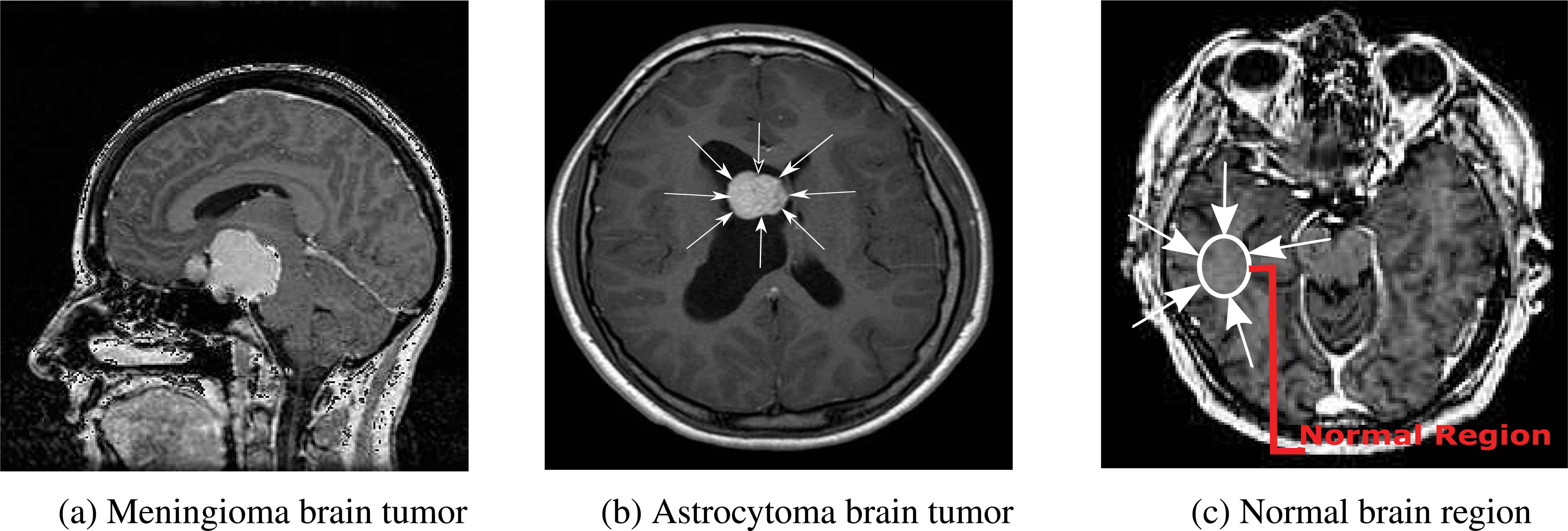
Different brain tumor classes
The main objective of this research is to articulate LAWs texture energy feature analysis [16] to describe the textural and spatial structural variations of tumor cells. MR images obtained from the internet database are salt-paper noise filled due to which the general feature extraction techniques (Gray Level Co-occurrence Matrix (GLCM), First Order Statistics (FOS) etc.) detect tumorous cells as normal cells. Laws texture energy measures (LTEM) is a combination of zero order, first order, and second order statistical analysis, therefore, it removes the ambiguities between tumorous and normal cells and can distinguish between these cells more accurately. The highlighted feature of this technique is the ability to detect micro-structure features (level, edge, spot, ripple, and wave) as well as global feature or macro features (energy, variance etc.) of the region of interest in an image in either one-direction or in bi-direction. The accuracy of LTEM is higher as it can detect textural energy (depends on the length of the mask chosen) in a particular direction.
The CAD system consists of three major parts: The ROIs selection, intensity and texture feature extraction, and classification of brain tumors based on ANN. The ROIs are marked in such a way that they cover both necrotic and cystic part of the tumor. The feature extraction includes First Order Statistics (FOS), Gray Level Co-occurrence Matrix (GLCM), Gray Level Run Length Matrix (GLRLM), LAWs Texture Energy Measure (LTEM), and Gabor Filters (GWT). These intensity and texture features play a crucial role in discriminating different brain tumor classes.
2. Background Theory
Many authors have proposed various algorithms for classification of brain tumors by developing various computer aided diagnostic (CAD) system based on different features and classification algorithm [1–4]. Generally, these systems use image processing techniques such as feature extraction, selection, and classification. The primary motive behind all these developed CAD systems is to achieve maximum accuracy. These systems used different types of brain tumor database such as MR spectroscopy, and echo planar maps related to cerebral blood volume (rCBV) along with MR imaging. The echo planar maps, MR images and MR spectroscopy are used for low grade and high grade brain tumor classification [5]. Along with these techniques, many a times MR image and perfusion data was also used for the same purpose [6, 7].
There are some of previous studies which determine the clinical importance of each MR sequence. A few tumorous regions of interest (ROI(s)) are marked and segregated by radiologists through a GUI developed by the authors. Many researchers have used different sizes of ROI(s) which has a considerable effect on the analysis [11, 12]. However, the optimal ROI size varies according to the feature extraction methodology and its final application. Therefore, it is essential to examine the influence of ROI size on texture analysis for brain tumor classification. The segregated ROI should have sufficient number of pixels which gives better information. The textural feature information is highly sensitive according to the number of pixels i.e. size of ROI [13]. At least 800 pixels are necessary in a selected ROI to obtain the reliable result of texture analysis [14].
These are some feature which depends on the neighbor pixels as Gray Level Run-Length Matrix (GLRLM), Gray Level Co-Occurrence Matrix (GLCM). Haralick, Shanmugum, R M K, and Dinstein I [15] introduced GLCM approach in 1973. The GLCM feature matrix is most commonly used in feature extraction by many researchers. 100 Features are also extracted by Zarchari et al. [17] where in these features are extracted from GLCM, intensity, Gabor, statistical, and shape based techniques.
Many studies have been already performed on multiclass brain tumor classification. Sachdeva et al. [18] took a dataset of 856 SROIs from 428 post-contrast T1 MR-images. A Principal Component Analysis (PCA) along with Artificial Neural Network (ANN) had been used which gave an overall accuracy of 85.23% and an individual class accuracy for Astrocytoma is 86.15%, Glioblastoma Multiforme is 65.10%, 63.36% for Medulloblastoma, 91.50% for Meningioma and for Metastases it is 65.21%. Zacharaki et al. [17] performed experiment on 98 images from which 100 features are extracted. The feature extraction process unit had Gabor, GLCM, intensity, shape and statistical techniques for obtaining features. An Accuracy of 91.7%, 90.9%, 41.2% and 33.4% is obtained for Metastatic, Low-Grade Glioma, Glioblastoma Multiforme and Glioma Grade III respectively. Georgiadis et al. [19] studied Glioma, Meningioma, and Metastatic brain tumors using Least Square Feature Transformed-Probabilistic Neural Network (LSFTPNN). A PNN classifier gave better results than other classifiers in terms of computational load and training. The output of LSFT is given as the input to PNN because of better pattern classification ability of LSFT. A dataset of 75 images of Glioma, Meningiomas, and Metastatic had been collected. An individual class accuracy of 96.67%, 95.24%, and 87.50% had been achieved for Gliomas, Meningiomas, and Metastates respectively. Al-Shaikhli et al. [10] performed a different study on a database which has 50 normal brain images, 50 Glioma brain tumor images, 50 Glioblastoma brain tumor images, and 50 images of Metastatic brain tumor. This database was experimented with dictionary learning and sparse coding classifier which has K-SVD algorithm. An overall accuracy of 93.75% was achieved with this method.
It is being observed that there are only few researchers who have done the classification of Meningioma and Astrocytoma together with Normal brain regions. Mostly researchers classified Glioma, Meningioma, and Metastatic brain tumors. These brain tumors are easily classified as they have distinctive features. Besides this, a very few features were extracted and as a result low accuracy were obtained. No attempts have been made to include LAW’s textural energy measures (LTEM) in feature extraction part to classify brain tumors. A very few studies have been done on classification of Meningioma and Astrocytoma brain tumors with lower classification accuracies due to their similar textural and intensity patterns.
In this papers, these above limitations are surmounted with the help of GUI developed for ROI segregation. 371 texture and intensity features are obtained from the ROI(s) extracted from the database of post-contrast T1 weighted MR-images of 10 patients. Initially, ANN classifier is used to test these ROI(s) with limited number of features excluding LTEM features. LTEM features are then added to obtain more accuracy with ANN classifier. Different experiments have been performed on these two experimental setup for three classes: Meningioma (MENI- Class 1), Astrocytoma (AST- Class 2) and Normal brain region (NORM class-3).
| S. No. | Author (Year) | Brain tumor classes | Number of Features | Individual Class Accuracy | Overall Classification Accuracy | |
|---|---|---|---|---|---|---|
| Brain Tumor | Accuracy | |||||
| 1. | Zarchari (2010) | Low Grade Gliomas, Glioblastoma Multiforme, Metastatic | 100 features from GLCM, Gabor, shape and statistical feature extraction techniques | Low-grade Gliomas | 90.9% | 72% |
| Glioblastoma Multiforme | 33.4% | |||||
| Metastatic | 91.7% | |||||
| 2. | Georgiadis (2008) | Metastases, Meningiomas Gliomas | 4 features from histograms, 22 features were extracted from the GLCM and 10 features were extracted from the run-length matrices | Metastases | 87.50% | 93.14% |
| Meningiomas | 95.24% | |||||
| Gliomas | 96.67% | |||||
| 3. | Sachdeva (2013) | Astrocytoma, Glioblastoma, Multiforme Medulloblastoma, Meningioma, Metastatic, Normal regions | 218 intensity and texture features | Astrocytoma | 90.74% | 85.23% |
| Glioblastoma Multiforme |
88.46% | |||||
| Medulloblastoma | 85% | |||||
| Meningioma | 90.70% | |||||
| Metastatic | 96.67% | |||||
| Normal regions | 93.78% | |||||
| 4. | Present study (2015) | Meningioma, Astrocytoma, Normal Brain | 371 intensity and texture features Using GLCM, GLRLM, GABOR, LTEM, FOS Techniques | Meningioma | 91.40% | 92.43% |
| Astrocytoma | 91.43% | |||||
| Normal Brain | 94.29% | |||||
Overview of the brief study on classification of brain tumors
3. Methodology
In this methodology, a CAD system has been developed as shown in Fig.2 to differentiate three types of brain tumors with higher classification accuracy. The CAD system developed by authors overcomes earlier limitations in multi-class classification of brain tumor. It dwells three main parts which are as following:
- 1.
Segregating ROI(s) from database
- 2.
Intensity and texture feature description
- 3.
ANN classifier with features as an input
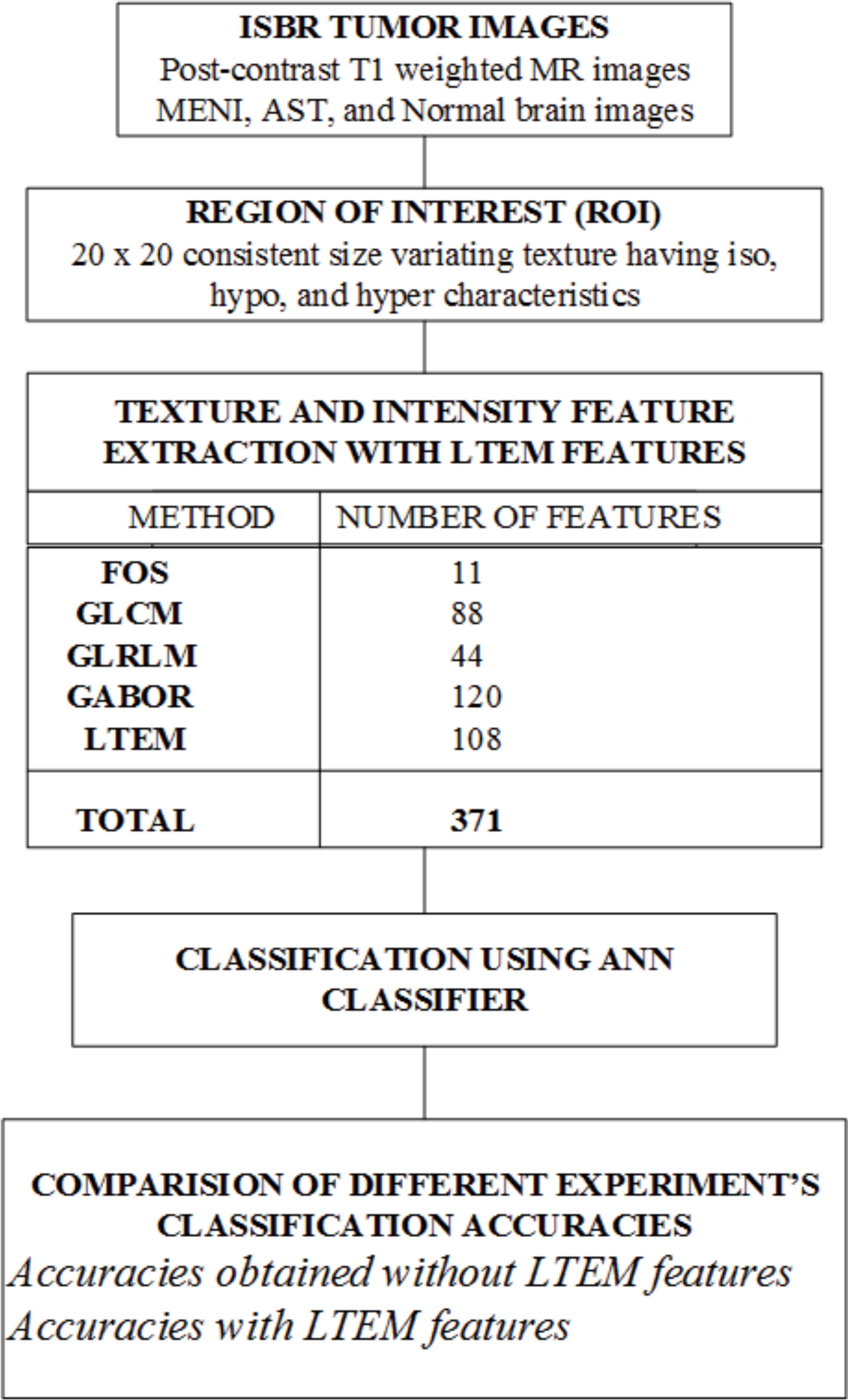
Block diagram of the developed CAD system
3.1. Segregating Regions of Interest (ROIs) from Database
A secondary database of ROI(s) is obtained by developing a GUI using MATLAB 2015a which guides the user to mark as well as segregate the region of interest from the main image. These ROI(s) are a sub part of main image in medical imaging. A ROI has the fundamental diagnosis information which can be used for computations and diagnosis process.
Depending on the methodology used, optimal size of the ROI varies. The ROI size also depends on the application for which it will be used. Either too large ROI like 40×40 or too small ROI like 10×10 does contain too much or too less information for computation respectively [14]. An average size of brain tumor is 30×30.
A comparative analysis has been performed on various sizes 40×40, 30×30, 20×20 of ROI(s) segregated from a particular image from database as shown in Fig. 3. This comparative analysis has been done on these ROI(s) which is based on plotting box plots in Matlab 2015a. These box-plots are based on two different features which are contrast and difference entropy. MENI (class-1) and AST (class-2) have been selected for comparison with two different ROI sizes. MENI-20 signifies Meningioma with ROI size 20×20 and AST- 20 means Astrocytoma with ROI size 20×20.
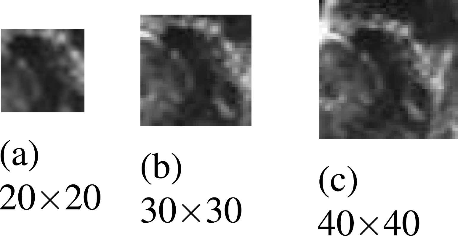
Various sizes of ROIs selected
It has been analyzed from this comparison that the differentiation capability of ROI size 20×20 and 40×40 is almost similar. Along with differentiating two classes, ROI size of 20×20 and 40×40 contains approximately similar information within itself. It is being analyzed from the Fig.4. that MENI-20 and MENI-40 have a dominance in lower range and AST-20 and AST-40 have dominance in upper part. The same type of tumors show similar information except for some typical cases as stated below. The major reasons for segregating 20×20 size ROI(s) are:
- •
ROIs are marked in such a way that they cover both necrotic and cystic (heterogeneous) part of the tumor.
- •
Few of the tumors show peripheral enhancement such as AST and thus cause change in the texture property of the periphery and in the region near to the periphery. ROI of 20× 20 thus cover both the hypo as well as hyper region.
- •
It provides less computational time and high differentiation capability.
Therefore, this size is found out to be appropriate for segregating ROI in this methodology.
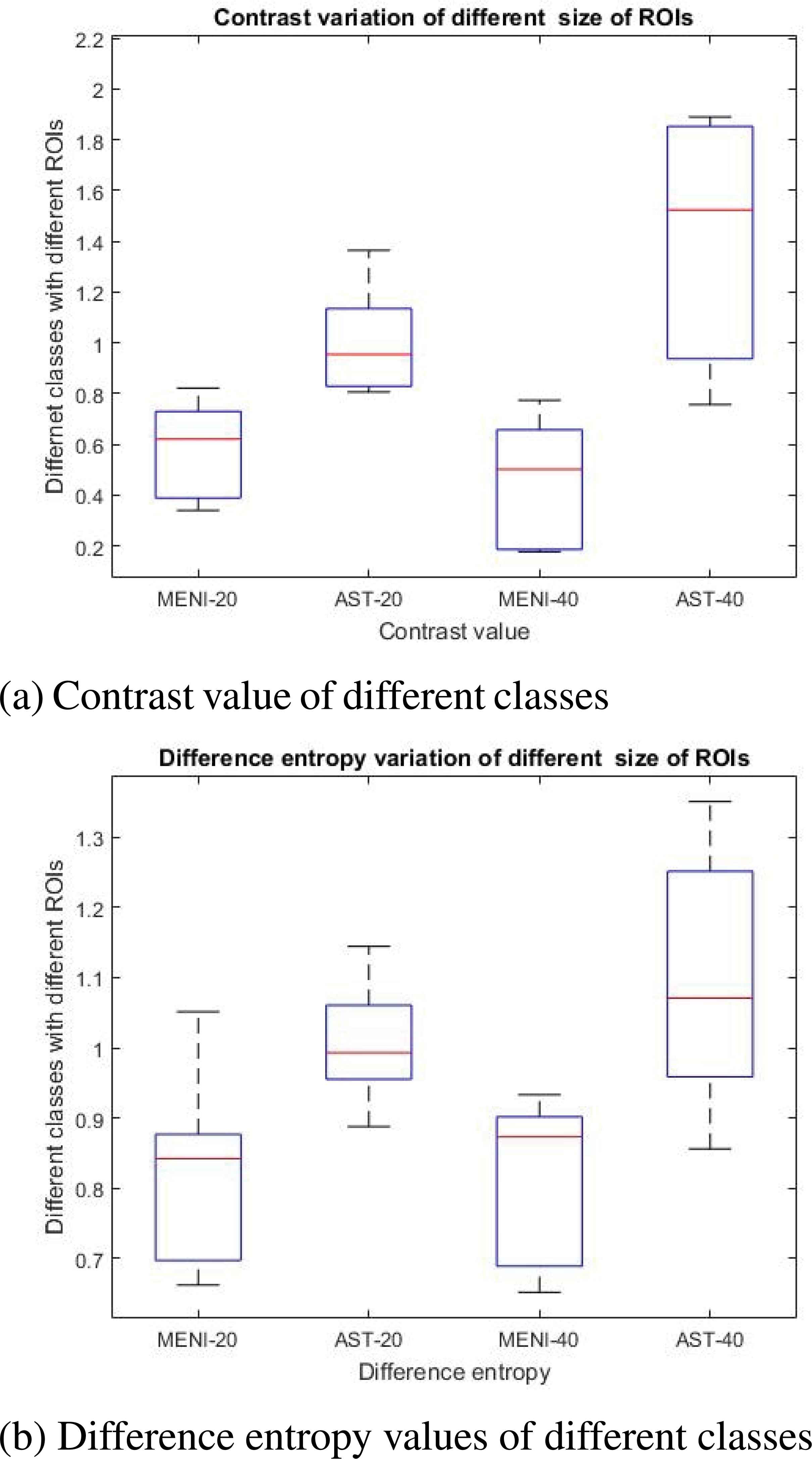
Box plot analysis of different parameters with dissimilar ROI sizes
3.2. Intensity and Texture Feature Description
The combination of intensities at a specific positions relative to each point in the image is named as features. The categorization of features depends on the number of features defining points of an image. These features are categorized into higher order, second order, and first order features, where higher number of feature defining points means higher order.
In the present method, ROI(s) are taken as input to feature extraction unit. Initially, five different intensity and texture features of higher, second and first order statistics, spatial-filtering with laws texture energy mask, and multi-scaled and multi-resolution tune-able analysis with Gabor wavelet are selected. These five methods are (i) First order statistics (FOS) (ii) Gray-level co-occurrence matrix (GLCM) (iii) Gray level run-length matrix (GLRLM) (iv) LAWS Texture energy measures (LTEM) and (v) Gabor wavelet (GWT). There are various studies [21, 22] in which a combination of these features has been used. The feature selection is based on these studies and the type of information it provides. A total of 371 visual and non-visual texture and intensity features are extracted and then applied to present classification CAD system. These methods have one extracted feature set for each hence total five feature sets are obtained from five methods. These sets were concatenate into one feature set named as feature vector. Further, this feature vector is used for characterization of image. These five textural features are:
3.2.1. First Order Statistics (FOS)
A total of 11 First order statistics (FOS) features are extracted. These features are minimum gray level, maximum gray level, mean gray level, median gray level, standard deviation of gray levels, coefficient of variation, gray level skew-ness, gray level kurtosis, gray level energy, gray level entropy, and mode gray level [23, 24].
3.2.2. Gray Level Co-occurrence Matrix (GLCM)
A GLCM matrix G(θ,d)(I1,I2) is being developed based on the occurrence of gray-levels that how frequently two pixels with gray-levels I1,I2 appear in the window separated by a distance (d) in direction(θ). The GLCM matrix G(θ,d)(I1,I2) is a function of two parameters: relative distance measured in pixel numbers (d) and their relative orientation (θ). The orientation (θ) is quantized in four directions that represent horizontal, diagonal, vertical and anti-diagonal by 0°, 45°, 90° and 135° respectively. The non-normalized frequencies of co-occurrence matrix as functions of distance (d) and angle 0°, 45°, 90° and 135° can be represented respectively as:
3.2.3. Gray Level Run-length Matrix (GLRLM)
The total number of Gray Level Run-Length Matrix (GLRLM) textural features which are extracted from GLRLM matrix is 44. The features which are extracted are short run emphasis, long run emphasis, low gray level emphasis, high gray level run emphasis, short run low gray level emphasis, short run high gray level emphasis, long run low gray level emphasis, long run high level emphasis, gray level non-uniformity, run length non-uniformity and run percentage are considered for analysis [26]. These 11 features are calculated in four different directions (0°, 45°, 90° and 135°) from GLRLM matrix to make a total of 44 features.
3.2.4. LAWS Texture Energy Measures (LTEM)
Laws texture energy features [27] [16] are obtained from special 1-D filters of different length. These special 1-D filters are represented as L5, E5, S5, W5, R5, L7, E7, S7, L9, E9, S9, W9, R9 depending upon their length and working. L, E, S, W, R stand for level, edge, spot, wave and ripple respectively and have different resolutions. The 1D filters described above are shown in Table 3. These filters are combined to form 59 different 2-D filters. Further, the segregated ROI (s) are convolved with the 2-D filters. As a result, 59 convolved output images are obtained. The obtained output images are passed through another stage which is known as “macro static”. These convolved images are used to extract three features viz. mean, variance, and energy.
| −1 | −2 | 0 | 2 | 1 |
| −4 | −8 | 0 | 8 | 4 |
| −6 | −12 | 0 | 12 | 6 |
| −4 | −8 | 0 | 8 | 4 |
| −1 | −2 | 0 | 2 | 1 |
(a) L5E5
| −1 | 0 | 2 | 0 | −1 |
| −2 | 0 | 4 | 0 | −2 |
| 0 | 0 | 0 | 0 | 0 |
| 2 | 0 | 4 | 0 | 2 |
| 1 | 0 | −2 | 0 | 1 |
(b) E5S5
| 1 | −4 | 6 | −4 | 1 |
| −4 | 16 | −24 | 16 | −4 |
| 6 | −24 | 36 | −24 | 6 |
| −4 | 16 | −24 | 16 | −4 |
| 1 | −4 | 6 | −4 | 1 |
(c) R5R5
| −1 | 0 | 2 | 0 | −1 |
| −4 | 0 | 8 | 0 | −4 |
| −6 | 0 | 12 | 0 | −6 |
| −4 | 0 | 8 | 0 | −4 |
| −1 | 0 | 2 | 0 | −1 |
(d) L5S5
Some of the most successful masks (These masks can be utilized in conjunction with E5L5, S5E5, and S5L5)
| Filter types | 1-D convolution filters | Number of 2-D mask generated from special 1-D filters (A) | Number of filter pairs having one filter in the pair identical to other if one of them is rotated by 90° (B) | Number of rotation invariant images (A-B) |
|---|---|---|---|---|
| Length 5 | L5= [1, 4, 6, 4, 1] | 25 | 10 | 15 |
| E5= [-1, -2, 0, 2, 1] | ||||
| S5= [-1, 0, 2, 0, -1] | ||||
| W5= [-1, 2, 0, -2, 1] | ||||
| R5= [1, 4, 6, -4, 1] | ||||
| Length 7 | L7= [1, 6, 15, 20, 15, 6, 1] | 9 | 3 | 6 |
| E7= [-1, -4, -5, 0, 5, 4, 1] | ||||
| S7= [-1, -2, 1, 4, 1, -2, -1] | ||||
| Length 9 | L9= [1, 8, 28, 56, 70, 56, 28, 8, 1] | 25 | 10 | 15 |
| E9= [1, 4, 4, -4, -10, -4, 4, 4, 1] | ||||
| S9= [1, 0, -4, 0, 6, 0, -4, 0, 1] | ||||
| W9= [1, -4, 4, 4, -10, 4, 4, -4, 1] | ||||
| R9= [1, -8, 28, -56, 70, -56, 28, -8, 1] | ||||
| Total | 59 | 23 | 36 | |
One-dimensional filters of lengths 5, 7, and 9 which are used in extraction of LAWs texture features and number of corresponding rotation invariant features
The overall features constitute 59 output filters from which 23 output filters are similar to those 23 output filters obtained at 90° rotation. The combination of any two textural energy image obtained from same pair is called rotation invariant image. For example, when a textural energy image obtained from S5W5 and W5S5 is combined than the image obtained is a rotation invariant image.
3.2.5. Gabor Wavelet Filter (GWT)
Gabor wavelets are a multi-scaled and multi-oriented filter [28, 29]. The principle reason of Gabor filter selection is its tuneable scale and orientation. This filter has a group of wavelets where each wavelet has some amount of energy at a particular direction and frequency. This energy is called localized energy or features. These Gabor filters are convolved with the ROI (s) to get the Gabor filtered output images. A total of 120 features namely mean, entropy and energy are calculated from these Gabor filtered output images with 5 scale and 8 orientations. A feature set of 120 is obtained from Gabor filtered output images.
3.3. Classification
It is a technique which is used for classification of input prototypes into equivalent analogous classes. There are many factors which affects the selection process of a classifier, those factors are: algorithm performance, classification accuracy and computation resources.
A conventional Artificial Neural Network (ANN) is a mathematical system which has nonlinear artificial neurons. An ANN can be multilayered ANN or single-layered ANN. Multi-layered ANN mostly has three layers: input, hidden, and output layer as shown in Fig. 5. The feature vector is given as an input to the input layer. The input layer has equal number of neurons as the number of features extracted i.e. feature vector length. An output layer with three neurons has selected as three brain tumor classes has to be classified. Every output layer neuron gives a ‘1’according to the label class defined for it and gives a ‘0’for another output neurons. The hidden layer neurons communicate between the output layer neurons and the external input layer neurons. A guess and check method is used to find the appropriate number of neurons for hidden layer. It was concluded after a number of trials that 18 number of neurons are suitable for classification and also for a fast convergence. The leave-one-out cross-validation is not used. The most intense computations take place in the training period. Once these computations are done, the testing and validation process will become relatively fast [30–31].
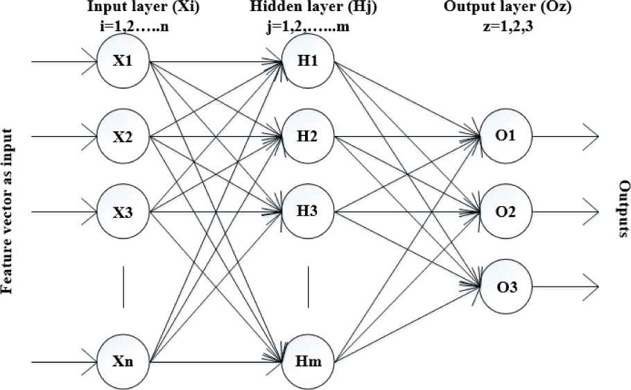
Internal architecture of an ANN system
A supervised learning is opted for this ANN classifier with back-propagation weight adjustment. Generally, there are two types of signal in this classifier. First is input signal which acts at the classifier input neurons. This input signal propagates forward towards hidden neuron layer and then finally reaches at the output neuron layer, then it is called output signal. Second signal is error signal which starts at the output layer and goes backward (layer by layer). The output of the ANN is:
4. Database and Software
The database and software details are described in the following section:
4.1. Database
The database used is of post-contrast T1 weighted MR images. These images are provided by Surgical Planning Laboratory, Departments of Radiology, Brigham and Women’s Hospital, Harvard Medical School, Boston, MA, USA [32, 33]. This database contains brain MR-images of Astrocytoma, Meningioma, and Glioma. All images are obtained using the same MRI equipment (Siemens Verio, Erlangen Germany, and 3 Tesla MR Scanner). From this database, 105 images of MENI (Class-1) & AST (Class-2) are taken. Gliomas are rejected due to the high salt and pepper noise on the images. The Normal regions (NORM-Class 3) are marked from these 105 images to have variant data of white matter and gray matter. T1 images are especially used to distinguish gray and white matter where gray matter is dark gray (iso to hypo), white matter is light gray (hyper). The normal region gets disarticulated due to spreading of the tumor and leakage of cerebrospinal fluid (CSF). The regions near to tumor are marked specifically as the ad-joint normal area shows a bit similar properties to that of tumor. Therefore, radiologists and neurosurgeons find it difficult to locate the exact boundary of tumor. Therefore, ROI(s) of the normal region are considered in this work. The tumor boundaries of MENI (Class-1), AST (Class-2) and NORM (Class-3) ROIs are marked by the expert radiologist in the present work and are taken as ground truth.
4.2. Software
This method is implemented in MATLAB 2015a and MR images of size 256×256 are taken for testing. This method is performed on notebook PC HP ENVY having 8 GB RAM with Intel(R) Core (TM) i5-4200 CPU@ 2.50 GHz.
5. Experimental Setup
The experiments performed are divided into four sets to test the performance and robustness of the proposed approach with other techniques as well. In the experimental setup, first two experiments symbolize the use of LTEM to increase the overall accuracy and individual class accuracy. In the third and fourth experiment, the proposed approach is compared with the previous study developed by Sachdeva et al. [18]. In the third experiment, feature reduction technique is used with the limited number of features as proposed by the author. In the fourth experiment, feature reduction technique with the addition of LTEM features in the feature set is applied.
Experiment 1:
Initially in this experiment, three tumor classes are classified using ANN approach without LTEM features. Training, validation and testing are the three stage used for multi-layer ANN classifier. Depending upon the stages of multi-layer ANN classifier, three sets of database has been built namely: training set, validation set, and testing set. Training set has 30% ROI (s) from each class. Validation set has 10% of ROI (s) from each class. As the validation process is completed, ANN optimizes its parameter and performs independent evaluation consisting of 60% of ROI(s) as a testing set. The dataset used for training is not repeated in testing i.e. random selection method has not been applied.
Structure of ANN classifier without LTEM features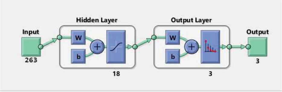
Experiment 2:
In the second experiment also, the dataset used for training is not repeated in testing i.e. random selection method has not been applied. A selection of 30% ROIs has been made for the training set from each class. The validation set has 10% ROIs from each class. As the validation process is completed, ANN sets all its parameters optimally fixed. Now, ANN is ready for independent evaluation of the test set which consists 60% ROIs.
Structure of ANN classifier with LTEM features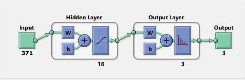
In this experiment, an analysis has been performed on the effect of LTEM features in classification of these ROIs with ANN classifier. The basic data structure used for evaluation is Confusion Matrix. Confusion matrix is the basic parameter for performance calculation of the developed CAD system. The confusion matrix is based on following parameters:
- •
True positive(TP) = Correctly identified in same class as positive cases
- •
False positive(FP) = Incorrectly identified in other class as negative cases
- •
True negative(TN) = Negative cases classified in same class correctly
- •
False negative(FN) =Incorrectly classified in other classes as positive cases
The performance of the ANN is also analysed in terms of individual class accuracy and overall classification accuracy. These parameters can be described as:
- •
- •
Experiment 3:
The objective of this experiment is to analyse other feature extraction techniques with same database used for experiment 1 and 2. For this experiment, training dataset is not repeated in testing i.e. random selection of data is not being chosen. For the training set 30% ROIs are selected for training set from each class. The validation set has 10% ROIs from each class. A total of 218 features are extracted which consists 16 features of Laplacian of Gaussian (LOG), 16 features of GLCM, 36 of rotation invariant local binary patterns (RILBP), 10 of intensity based features (IBF), 100 of direction Gabor texture features (DGTF), 40 of rotation invariant circular Gabor features (RICGF). A feature reduction technique, Principle component analysis (PCA) is applied with ANN classifier. The feature reduction technique is used to reduce the dimensionality of the feature set. The reduction of the feature set provides improved results.
Experiment 4:
In the fourth and last experiment also, available dataset is used. The dataset used for training is not repeated in testing i.e. random selection method has not been applied. A selection of 30% ROIs has been made for the training set from each class. The validation set has 10% ROIs from each class. As the validation process is completed, ANN sets all its parameters optimally fixed. Now, ANN is ready for independent evaluation of the test set which consists 60% ROIs. For this experiment, PCA is applied on 371 features as described in experiment 2. The evaluation of this experiment is done using confusion matrix.
6. Results and Discussion
Experiment 1:
Initially, in this experiment, three tumor classes are classified using ANN approach without LTEM features. A feature bank consisting FOS, GLCM, GLRLM, and GWT features (a total of 263 features) is taken as an input to the multi-layer ANN classifier. Three different classes viz. MENI (Class-1), AST (Class-2), and NORM (Class-3) are classified. An overall classification accuracy of 78.10% is being observed as given in Table 4. Individual class accuracy for MENI (class-1) is 77.14%, 74.30% for AST (class-2), and 82.86% for NORM (class-3). Training, validation and testing are the three stage used for multi-layer ANN classifier. Depending upon the stages of multi-layer ANN classifier, three sets of database has been built namely: training set, validation set, and testing set. Training set has 30% ROI (s) from each class. Validation set has 10% of ROI (s) from each class. As the validation process is completed, ANN optimizes its parameter and performs independent evaluation consisting of 60% of ROI(s) as a testing set. It is being observed from Table 3 that the MENI (Class-1) is highly misclassified with AST (Class-2) and vice-versa as AST (Class-2). MENI (Class-1) is 20% misclassified with AST (Class-2). The higher misclassification between these two classes is due to the hypo as well as hyper intense nature of AST (Class-2) and the cystic and necrotic components in the ROIs.
| Experiment 1 results of ANN classifier without LTEM | |||
|---|---|---|---|
| Class | MENI (Class-1) | AST (Class-2) | NORM (Class-3) |
| MENI (Class-1) | 27 | 6 | 2 |
| AST (Class-2) | 7 | 26 | 4 |
| NORM (Class-3) | 1 | 3 | 29 |
| Individual classification accuracy | 77.14% | 74.30% | 82.86% |
| Overall classification accuracy 78.10% | |||
Confusion Matrix of Experiment 1
Experiment 2:
An accuracy of 77.14% for MENI (Class-1), 74.30% for AST (Class-2), and 81.81% for NORM (Class-3) has already been delivered in previous experiment. An addition of LTEM features has been done in the feature bank with FOS, GLCM, GLRLM, and GWT features (a total of 371 features). These features are taken as input to the multi-layer ANN classifier. An overall classification accuracy of 91.43% is being observed as shown in Table 5. Individual class accuracy for each class is 91.40% for MENI, 91.43% for AST, and 94.29% for NORM. Training set has 30% ROI (s) from each class. Validation set has 10% ROI (s) from each class. As the validation process is completed, ANN sets all its parameters optimally fixed. Now, ANN is ready for independent evaluation of the test set which consists 60% ROI (s). It is observed from Table 5 that the misclassification between MENI (Class-1) and AST (Class-2) has been reduced. An improvement of 12% has been observed from the Table 5 as initially the misclassified between MENI (Class-1) and AST (Class-2) is 20% but after addition of LTEM features the misclassification between these two classes is 8%. This improvement in classification has been achieved with the help of LTEM features as it can detect fundamental texture patterns viz. level, spot, wave, ripple, and edge. It is also been observed that the LTEM features can clearly differentiate MENI (Class-1) and AST (Class-2) despite of necrotic and cystic components, location and size of the tumors. More than 30% ROI in training stage can further improve the individual classification accuracy as well as overall classification accuracy.
| Experiment 2 results of ANN classifier without LTEM | |||
|---|---|---|---|
| Class | MENI (Class-1) | AST (Class-2) | NORM (Class-3) |
| MENI (Class-1) | 32 | 2 | 1 |
| AST (Class-2) | 3 | 32 | 1 |
| NORM (Class-3) | 1 | 1 | 33 |
| Individual classification accuracy | 91.40% | 91.43% | 94.29% |
| Overall classification accuracy 92.43% | |||
Confusion Matrix of Experiment 2
Experiment 3:
The feature bank has 218 features of LOG, GLCM, RILBP, IBF, DGTF, and RICGF. Feature reduction technique- Principle component analysis (PCA) is applied with ANN classifier. The feature reduction technique is used to reduce the dimensionality of the feature set. Three different classes viz. MENI (Class-1), AST (Class-2), and NORM (Class-3) are classified with the above technique. The feature set of 218 features is given as input to PCA and as an output, a reduced set of features is obtained which is an input to ANN. An overall accuracy of 81.90% can be observed from Table 6. The individual class accuracy for MENI (class-1) is 80%, 77.14% for AST (class-2), and 88.57% for NORM (class-3) is obtained. It is being observed from Table 6 that the MENI (Class-1) is highly misclassified with AST (Class-2) and vice-versa as AST (Class-2). MENI (Class-1) is 17.14% misclassified with AST (Class-2). The higher misclassification between these two classes is due to the hypo as well as hyper intense nature of AST (Class-2) and the cystic and necrotic components in the ROIs.
| Experiment 3 results of PCA-ANN classifier without LTEM | |||
|---|---|---|---|
| Class | MENI (Class-1) | AST (Class-2) | NORM (Class-3) |
| MENI (Class-1) | 28 | 5 | 1 |
| AST (Class-2) | 6 | 27 | 1 |
| NORM (Class-3) | 1 | 3 | 33 |
| Individual classification accuracy | 80.00% | 77.14% | 88.57% |
| Overall classification accuracy 81.90% | |||
Confusion Matrix of Experiment 3
Experiment 4:
The feature bank has 371 features similar to experiment 2. A feature reduction technique-Principle component analysis (PCA) is used with ANN classifier. Three different classes viz. MENI (Class-1), AST (Class-2), and NORM (Class-3) are classified with the above technique. The feature set of 371 features is given as input to PCA and as an output, a reduced set of features is obtained which is utilized as an input to ANN. An overall accuracy of 93.34% can be observed from Table 6. The individual class accuracy for MENI (class-1) is 94.29%, 94.29% for AST (class-2), and 91.43% for NORM (class-3) is obtained. It is observed from Table 6 hat the misclassification between MENI (Class-1) and AST (Class-2) has been reduced. An improvement of 2.89% has been observed from the Table 7. In experiment 1 the misclassified between MENI (Class-1) and AST (Class-2) is 20%. After the addition of LTEM features the misclassification between these two classes is 8% in experiment 2. In experiment 3, the misclassification between these two classes is 17.14%. In experiment 4, this misclassification rate is almost 3% which is quite low. This improvement in classification has been achieved with the help of LTEM features with PCA-ANN classifier as it can detect micro and macro features of the image. It is also observed that the LTEM features can clearly differentiate MENI (Class-1) and AST (Class-2) despite of necrotic and cystic components, location and size of the tumors.
| Experiment 4 results of PCA-ANN classifier with LTEM | |||
|---|---|---|---|
| Class | MENI (Class-1) | AST (Class-2) | NORM (Class-3) |
| MENI (Class-1) | 33 | 1 | 1 |
| AST (Class-2) | 1 | 33 | 2 |
| NORM (Class-3) | 1 | 1 | 32 |
| Individual classification accuracy | 94.29% | 94.29% | 91.43% |
| Overall classification accuracy 93.34% | |||
Confusion Matrix of Experiment 4
7. Conclusion
An adequate computer aided diagnosis (CAD) system has been developed with additional features and improved accuracy for classification of brain tumors. The performance of this CAD system has been analysed through ANN classifier with a multifarious database of real post contrast T1-weighted MR-images. This database consisted of 20×20 size ROIs of primary brain tumors namely MENI (class 1), AST (class 2) and NORM (class 3). Total 371 texture and intensity features are extracted from these ROIs. Artificial neural network (ANN) has been used to classify these three classes as it provided better results with individual class accuracy and overall classification accuracy. The four discrete experiments have been performed with different feature set and classifiers. In the first experiment, 263 features are extracted and an overall classification accuracy of 78.10%, however it was noticed that MENI (class 1) was highly misclassified with AST (class 2). In experiment 2, 371 features were taken along with LTEM features. The improved individual classification accuracy of 91.40% was obtained for MENI (class 1), 91.43% for AST (class 2), and 94.29% for NORM (class 3) and an overall classification accuracy of 92.43% was achieved. It was noted from Table 5 that misclassification rate is quite low for MENI (class 1). In third experiment, a PCA-ANN technique was applied, where 218 features were extracted and were reduced by using PCA. An overall classification accuracy of 81.90% was achieved. However, the overall accuracy of experiment 3 is less than experiment 2 in spite of having a feature reduction technique (PCA). PCA along with the proposed feature set is used for experiment 4. It is observed that there is 1% increase in overall classification accuracy (Table 7). Further, it is noticed that addition of LTEM features has given better results whether used with or without feature reduction technique. The texture patterns obtained by adding LETM features, differentiated well between MENI (class1) and AST (class 2) despite of necrotic and cystic component, location, and size of tumor. This is due to their inherent property of detection of fundamental texture features such as level, edge, spot, wave and ripple in both horizontal and vertical directions which boosted the texture energy. Grouping micro-texture with macro-texture feature is a healthier approach to determine each minute details of the texture difference. This removes ambiguities between tumorous and normal cells and distinguishes between these cells more accurately. The L5E5 mask obtained is invariant to the illumination tilt in the image which detects iso-intense cells accurately. Overall, an improved CAD system by experimentation has been developed for the young and inexperienced radiologists as well as medical students.
References
Cite this article
TY  - JOUR
AU  - Puneet Tiwari
AU  - Jainy Sachdeva
AU  - Chirag Kamal Ahuja
AU  - Niranjan Khandelwal
PY  - 2017
DA  - 2017/01/01
TI  - Computer Aided Diagnosis System-A Decision Support System for Clinical Diagnosis of Brain Tumours
JO  - International Journal of Computational Intelligence Systems
SP  - 104
EP  - 119
VL  - 10
IS  - 1
SN  - 1875-6883
UR  - https://doi.org/10.2991/ijcis.2017.10.1.8
DO  - 10.2991/ijcis.2017.10.1.8
ID  - Tiwari2017
ER  -