
Diabetes Classification using Radial Basis Function Network by Combining Cluster Validity Index and BAT Optimization with Novel Fitness Function
- DOI
- 10.2991/ijcis.2017.10.1.17How to use a DOI?
- Keywords
- Radial Basis Function Networks; Classification; Medical Diagnosis; Diabetes; Optimal number of clusters; Bat Algorithm
- Abstract
Diabetes is one of the foremost causes for the increase in mortality among children and adults in recent years. Classification systems are being used by doctors to analyse and diagnose the medical data. Radial basis function neural networks are more attractive for classification of diseases, especially in diabetes classification, because of it’s non iterative nature. Radial basis function neural networks are four layer feed forward neural network with input layer, pattern layer, summation layer and the decision layer respectively. The size of the pattern layer increases on par with training data set size. Though various attempts have made to solve this issue by clustering input data using different clustering algorithms like k-means, k-medoids, and SOFM etc. However main difficulty of determining the optimal number of neurons in the pattern layer remain unsolved. In this paper, we present a new model based on cluster validity index with radial basis neural network for classification of diabetic patients data. We employ cluster validity index in class by class fashion for determining the optimal number of neurons in pattern layer. A new convex fitness function has also been designed for bat inspired optimization algorithm to identify the weights between summation layer and pattern layer. The proposed model for radial basis function neural network is tested on Pima Indians Diabetes data set and synthetic data sets. Experimental results proved that our approach performs better in terms of accuracy, sensitivity, specificity, classification time, training time, network complexity and computational time compared to conventional radial basis function neural network. It is also proved that proposed model performs better compared to familiar classifiers namely probabilistic neural network, feed forward neural network, cascade forward network, time delay network, artificial immuine system and GINI classifier.
- Copyright
- © 2017, the Authors. Published by Atlantis Press.
- Open Access
- This is an open access article under the CC BY-NC license (http://creativecommons.org/licences/by-nc/4.0/).
1. Introduction
Diabetes is a metabolic and hereditary disease that causes due to deficiency of insulin hormone in human body. Insulin plays key role in conversion of food into energy. Lack of sufficient insulin causes presence of excess sugar levels in the blood. As a result the glucose levels in diabetic patients are more than normal ones. Many people referred diabetes as Diabetes Mellitus (DM). It has symptoms like frequent urination, increased hunger, increase thirst and high blood sugar. Diabetes is the fastest rising long-term illness condition that impacts lots of people globally. The excess blood sugar within the blood vessels can harm the blood vessels, this kind of situation leads to a various complications like cardiovascular damage, kidney damage, nerve damage, eye damage and stroke.1 World Health Organization (WHO) statistics shows diabetes contributied major share in Non Communal Disease (NCD) deaths across worldwide population.2
Classification and predictive systems are actually reliable in the health care sector to explore hidden patterns in the patients data. These systems aid, medical professionals to enhance their diagnosis, prognosis along with remedy organizing techniques. A lot of studies revealed that Radial Basis Function Network (RBFN) helpful for classification and pattern recognition tasks. The performance of these neural networks are on par with the more widely used logistic regression model and Multi Layer Perceptron Network (MLPN) model. Moreover, these RBFNs are adaptive in nature and good at modeling nonlinear data.
MLPNs are most popular techniques for classification and use iterative process for training. Contrary to MLPNs, RBFNs are trained in single iteration and learn applications quickly. Thus, RBFNs drawing researchers attention for classification tasks. This RBFN network is made up of four layers namely input layer, pattern layer, summation layer and decision layer.3
The size of the input layer is determined by the dimensionality of training patterns and summation layer is by number of distinct classes in training patterns. To figure out number of neurons in the pattern layer, the simplest and most common method is to assign a neuron for each training pattern. Though this process is simple, it is not practical since most applications find numerous training patterns and the dimensionality of data is huge. So, usually it is a good practice to cluster the training patterns first to create a reasonable number of groups by employing clustering techniques such as k-means, k-medoids, SOFM, etc. Once we create a group we can assign a neuron to each group (cluster).4
In the process of identifying the number of groups in a given data, there is a problem of having different class data into one cluster as shown in fig 1. Especially at the cluster center locations near line of separation. This unbalanced clustering affect the performance of the RBFN network. To avoid this we can better take advantage of the information of class label while clustering the training patterns. It means, cluster the training patterns class by class instead of the entire patterns at the same time.5 This approach reduces the computation time for clustering training patterns compared to clustering entire patterns. It is because of less number of patterns in former approach.
Different groups of data inside the cluster center location near line of separation.
As a way to identify the pattern layer of an RBFN we need to fix a number of neurons from each class along with their radial basis function characteristics. Normally these radial basis functions are gaussian functions. A gaussian is usually characterized by it’s center location and shape (spread). To find these center locations for gaussian functions earlier so many attempts made by using clustering techniques. Mostly the k-means clustering process is used to locate a set of k gaussian function centers because of it’s simplicity to implement and also it runs only in O (nkt), where n is the size of the data, k is the no of clusters, and t is the no of iterations needed for algorithm convergence.6 These clustering algorithms partition the input data into k disjoint clusters. Once membership of all data points are determined, average of cluster elements is treated as the center and variance of cluster elements is treated as shape of corresponding cluster. These center and variance of each cluster is given as inputs to corresponding gaussian functions.
1.1. Radial Basis Function Network (RBFN) Model
Radial basis function network is an artificial neural network that uses radial basis functions as activation functions. The RBFN3 is a four layer feed forward architecture as shown in Fig. 2. The construction of this type of network involves determination of number of neurons in four layers. The detailed description of four layer architecture is as follows:
- •
Input layer: This layer contains D number of neurons, where D is input pattern dimension. This layer is fully connected with pattern layer.
- •
Pattern layer: This layer is made up of H (H < N) number of neurons, where N is the number of training patterns. This pattern layer is fully connected with summation layer. Every neuron of pattern layer is mathematically described by a gaussian radial basis function as follows.
Where- i
is the distinct class number in data,
- P
is the maximum number of classes,
- j
is the cluster number inside the class,
- Qi
is the maximum number of clusters inside the ith class,
- x
is the pattern presented at the input layer,
- μij
is the mean vector of jth cluster in ith class and
- σij
is the cluster variance (spread) of jth cluster in ith class.
Pattern layer is having gaussian activation functions. These gaussian functions are characterized by their mean vectors (centers) μij and shapes (spreads) σij of the clusters. The links joining the input layer neurons to the pattern layer neurons are direct connections with no weights.
- •
Summation layer: This layer has small number of neurons, with linear activation functions. Size of this layer is limited to number of distinct classes in the training data. Output of the kth neuron in summation layer given by Eq. (3).
Where
-
is weight between φij neuron in pattern layer to kth neuron in summation layer and
- Sk
is the output of kth summation layer neuron.
-
- •
Four layer architecture of RBFN for classification task.
1.2. Cluster Validity Indices
In k-means criteria, it is really hard to pre-determine value of k, i.e number of clusters inside the data. So we need a metric for the partitioning result in order to find the perfect number of clusters. Usually, clustering outcome is tested with a qualifying measure called cluster validity index. This validity index measures precisely how well the clustering splits the given data.
Several validity indices are introduced in literature. These indices are commonly combined with the clustering technique to have the overall finest intra-compact clusters and well separated inter clusters. Indices used in our experiments are discussed as follows:
1.2.1. Intra-Inter ratio validity index
Ray and Turi has introduced simplest validity index using intra-cluster and inter-cluster distances in order to search optimal quantity of clusters inside color image segmentation.6 The Intra-Inter validity index defined as follows
- i
= 1, 2, …,k-1,
- j
= i + 1, i + 2, …,k,
- zi
denotes the center of the cluster ci,
- k
is the number of the clusters and
- N
is the number of data points.
Intra-inter validity index needs to be minimized for better clusters. It means that smaller value for index indicates, intra clusters are compact and inter clusters are well separated.
1.2.2. Dunn validity index
Dunn index8 is another type of cluster index, it is treated as a modified version of intra-inter index. Dunn index definition is as follows:
Where
is the dissimilarity function between clusters ci and cj defined in Eq. (10)
is the cluster diameter defined in Eq. (11)
Dunn index needs to be maximized to identify compact and well-separated clusters. In other words, highest value for Dunn index indicates a good estimation of fine-tune cluster number.
1.2.3. Dynamic validity index
Above two indices are very sensitive to noise in the datasets and not suitable for complex data sets like DNA microarray dataset. J. Shen et al.8 have proposed new index called Dynamic Validity (DV) index to get a perfect cluster number to overcome above two problems. The dynamic validity index is represented as
- zi
is the center of the cluster Ci,
- N
is the number of data points and
- K
is the upper bound on number of clusters.
Modelling parameter Δ is used to control the noise in the data. Usually it’s value sets to 1 if there is no noise in the data and sets to less than 1 if there is some noise. It’s value sets to greater than 1 in some special cases like to create more compact clusters rather than well separated cluster. In other words, for which cluster number the DV Index reaches a minimum value that indicates the optimal number of clusters for a given data set.8
The organization of the rest of the paper is as follows. In section 2, literature survey related to the problem has been presented. Section 3 discusses about the proposed methodology. Section 4 explains about experimental outcomes that confirm the performance of the proposed methodology. In section 5, we have drawn some final conclusions based on experimental observations.
2. Background and Related Work
In medical diagnosis, classification and decision support systems are extensively used by medical experts and doctors. These decision support systems extract meaningful information from given medical data. This will help doctors to improve their prognosis and diagnosis procedure to provide better planning for treatment. In recent years, many studies have been performed on the diagnosis of diabetic disease. M. Koklu et al.9discussed three classifiers namely J.48, Bayes classifier and MLPN experimented on Pima Indians data set and among them Bayes classifier achieved best accuracy. Multiple Knot Spline Smooth Support Vector Machine (MKSS-SVM) has been used by W. Purnami et al.10 to improve the accuracy over smooth support vector machine for classifying Pima Indian diabetic patients data.
O. Soliman et al.11 have used a Least Squares Support Vector Machine (LS-SVM) along with modified version of Particle Swarm Optimization (PSO) algorithm for SVM parameter tuning to classify Pima Indian diabetic patients data. M. Bozkurt et al. have experimented using pima Indians dataset on eight classifiers namely Learning Vector Quantization (LVQ), Probabilistic Neural Network (PNN), Cascade-Forward Networks (CFN), Distributed Time Delay Networks (DTDN), Time Delay Networks (TDN), Feed Forward Networks (FFN), Artificial Immune System (AIS) and the Gini algorithm.12
M. Fiuzy et al.13 have introduced a new method for accurate diagnosis of diabetes through combination of fuzzy systems, evolutionary algorithms and artificial neural networks. R. Radha et al.14 used fuzzy computational paradigm for diagnosing diabetes related diseases by using inference rules inferred from physicians medical knowledge. A. Karegowda et al.15 have implemented a hybrid model for diagnosis of diabetes mellitus with Genetic Algorithm (GA) and Back Propagation Network (BPN), where Genetic Algorithm is used for obtaining connection weights of BPN.
A hybrid model of MLPN using fuzzy logic have been used by M. Khashei et al.16 in order to reduce the misclassification rate. Experimental results proved that hybrid model is better than other individual classification models. P. Jeatrakul et al.17 reviewed the performance of five neural network based classifiers namely general regression neural network, back propagation neural network, PNN, RBFN and complementary neural networks on Pima indians data set.
Y. J. Oyang et al.18 have used a novel kernel density estimation function to reduce the construction time of RBFN. P. Venkatesan et al. 19 used RBFN for prediction of diabetes mellitus and also compared performance of RBFN with MLPN and logistic regression using dataset size of 600 records are collected from local hospital. Shankaracharya et al.20 outlined recent advances and potentials in machine learning algorithms on diabetes diagnosis tools and reviewed nearly 30 approaches based on machine learning systems using Pima Indians diabetes data set.
Size of the hidden layer increases on par with training data set size. To resolve this problem many researchers have suggested clustering of input data. In literature, clustering techniqes such as fuzzy c-means21, Conditional Fuzzy Clustering algorithm 22, enhanced LBG23, k-means24, Clustering for Function Approximation method 25 and the Alternating Cluster Estimation method 26 etc. have been applied to address the above problem. The clustering procedure gets the cluster centers by trying to minimize the total squared error incurred in representing the data set by the different cluster centers. In order to find compact intra clusters and well separated inter clusters R. Siddheswar et al. 6 have introduced intra-inter ratio index and J. shen et al. 8 have introduced Dunn index and Dynamic Validity indices.
K. Ganapathy et al.33 have used a new Optimum Steepest Descent based Higher level Learning Radial Basis Function Network (OSDHL-RBFN) to handle improper center selection in complex real world problems. D. P. Ferreira Cruz et al.34 have proposed a bee-inspired clustering algorithm for RBFN design. In addition to this a heuristic method is used to select centers and dispersions for radial basis functions.
3. Proposed Methodology
This section presents our approach to find the number of neurons required for pattern layer in RBFN. Usually cluster validity indices are used to find the best cluster regions within the given data based on whether the cluster validity index is high or low (depends on validity index). The proposed model integrates cluster validity index with k-means clustering algorithm and this integrated k-means clustering algorithm is applied over data in class by class fashion, i.e integrated k-means is applied inside each class data. Where as in, direct approach k-means clustering algorithm is applied over the whole data set.
The proposed model presented in Fig. 3 consists of construction phase and evaluation phase. It uses integrated k-means algorithm to obtain fine tune cluster locations inside each class to determine pattern layer neurons during the construction phase. This determined pattern layer neurons along with input layer neurons (determined by dimensionality of patterns), summation layer neurons (determined by number of distinct classes in data) and one decision layer neuron are collectively used for the construction of proposed RBFN. Initially this RBFN has no weights between pattern and summation layers. These weights can be directly calculated using matrix inversion method, but as the data set grows this method is computationally expensive and also has matrix singularity problem.
Block diagram of proposed model.
Pseudo code for the ModelConstruction
Hence, in this paper a bat inspired optimization technique with novel fitness function has been proposed for finding the weights between pattern layer and summation layer. The above procedure for construction phase is summarized using pseudo code in Algorithm 1. During the evaluation phase, the constructed RBFN (by using Algorithm 1) is fed with test data to obtain the predicted pattern. This predicted pattern has values between 0 and 1. These values will be transformed into either 0 or 1 using threshold cut-off of 0.5. This transformed predicted pattern along with target pattern helps to evaluate the constructed model in terms of accuracy, sensitivity and specificity. The above procedure for evaluation phase is summarized using pseudo code in Algorithm 2.
Pseudo code for PredictClassLabel
3.1. Determination of Summation Layer Weights by Bat Optimization Algorithm (BA)
The Bat Algorithm (BA)27 has been successfully applied to various hard optimization problems. It has been proved that BA outperforms genetic and particle swarm algorithms. Most BA implementations in literature attracted us for weight determination of neural network. The BA algorithm simulates the behavior of bats. Bats are animals possessing the echolocation feature. These animals emit a series of short, high-frequency sounds and listen for the echo that bounces back from the surrounding objects and listen to the echoes. These echoes locate and identify the size, shape, direction, distance, and motion of the objects (prey). As the bat flies near its prey, the loudness decreases and rate of pulse emission increases.
Every bat is assigned a set of parameters that include pulse rate, velocity, position, loudness and frequency. Fine tuning of these parameters impact the convergence time and quality of solution.27 The basic principle of bat algorithm explained in detail is as follows:
3.1.1. Frequency, velocity and position representation
Bat Algorithm starts by randomly initializing a population of bats, where each bat has a velocity Vi, position Wi, fixed frequency Qmin with varying wavelength and loudness searching for prey. The pulse rate and frequency are adjusted automatically as they come closer to their targets. In a d-dimensional search space, at time t, the rules for updating positions Wi ad Vi are given by Eq. (22)–Eq. (24).
Where β ∈ [0,1]. Here W∗ is the current global best solution obtained by comparing all bats fitness values (choose minimum value). Qmin and Qmax values are chosen based on specific problem type, in our implementation we have used Qmin=10 and Qmax=30. Initially each bat is assigned with randomly generated frequency values from [Qmin, Qmax].
For the local search part, once we obtain the best solution among current best solutions, a new solution for each bat is generated using Eq. (25).
Where ε ∈ [−1, 1] and At is the average loudness value of all the bats at time t.27,28
3.1.2. Loudness, pulse rate representation
The loudness of sound (A) also takes range of values between the maximum loudness and minimum loudness. When the bat approaching near to the target usually its loudness value decreases and rate of pulse emission increases. In this work, we set the maximum loudness (Amax) equal to 2 and the minimum loudness (Amin) equal to 1. Loudness Ai and the rate of pulse emission ri are updated as per Eq. (26) and Eq. (27).
Where α and γ are constants with 0<α<1 and γ>0 values. We have used α=γ=0.9 in our simulations.28,29
3.1.3. New convex fitness function representation
Squared Error (SE) criteria is the most popular choice of fitness function for training the Artificial Neural Networks (ANN). Though SE is popular, as the gradient vanishes SE criterion suffers from local optimum problem. Hence in this work, we proposed a novel fitness function for bat algorithm based on modified entropy and modified cross entropy.
These cross entropy and entropy are defined in Eq. (28) and Eq. (29) respectively. where t is the target pattern, p is the predicted pattern and n is the size of training data set. We are trying to evaluate how well p fits the target t using cross entropy.
Pseudo code for Bat Algorithm (BA).
For every weight pattern (weight vector) model outputs the corresponding predicted pattern. During the model training, we evaluate cross entropy between target pattern and predicted pattern by varying weight pattern. Hence, fitness function f is a function of predicted pattern p. Which is given by Eq. (30) as follows:
If the cross entropy ((H(t, p)) is closer to the entropy of t ((H(t)), then p is the better approximation for t. When t = p, the cross entropy is simply the entropy of t and fitness function value becomes zero, which is a minimum value. As a whole we try to minimize the new convex fitness function f(p) value in order to get approximate weights for RBFN summation layer. In Algorithm 3, we explained in detail about bat optimization algorithm.
Theorem 1.
The proposed function f(p) is convex.
Proof.
We know that if f(p) is convex then the second derivative f″(p) is ≥ 0 for all p ∈ [0 1].
Let
H(t,p), H(t) are given Eq. (28) and Eq. (29),
We can write f (pi) as
As the target probabilities are fixed during the model training so the term
The first derivative of f (pi) is given by
Second derivative of f (pi) is given by
As 0≤ ti ≤ 1, 0≤ pi ≤ 1 and C is a positive constant so value of f″(pi) ≥ 0 for all values of pi.
Hence the function f(p) is convex □.
Theorem 2.
The proposed function f(p) is continuous.
Proof.
We know that polynomial and exponential functions are continuous everywhere. And if the function h and g are continuous at c then h.g is continuous at c.
The convex fiteness function f(p) is the composition of two functions: h(p) =ep and g(p) = 1-p. Both of these functions are continuous everywhere, so f(p) is continuous everywhere.
Hence the function f(p) is continuous □.
4. Experimental Results
4.1. Experimental Setup
The proposed model has been experimented using both bench mark Pima Indians Diabetes (PID) data set and synthetic data sets. The PID data set is taken from UCI machine learning repository.32 All the experiments are conducted using Matlab R2015a tool on system with RAM size of 8 Gb and Intel i7 processor speed of 3.6 GHz. We have used measures like classification accuracy, sensitivity, specificity, complexity, computational time, training time and classification time to evaluate the performance of the proposed model. Except Δ parameter, all parameters listed in Table 1 have been used in Bat Algorithm (BA) initialization and Δ parameter (in case of DV Index) is used for regulating noise in dataset.
| S.No | Parameter | Value | Explanation |
|---|---|---|---|
| 1 | Δ | 1 | Noise parameter for DV index |
| 2 | A | [1 , 2] | Sound Loudness |
| 3 | r | [0 ,0.1] | Pulse Rate |
| 4 | Qmin | 10 | Minimum frequency |
| 5 | Qmax | 30 | Maximum frequency |
| 6 | Bmax | 40 | No. of Bats |
| 7 | Imax | 250 | Maximum Iterations |
| 8 | γ | 0.9 | Increment Value of Pulse Rate |
| 9 | α | 0.9 | Decrement Value of Loudness |
Parameter values used in experiments.
4.2. Pima Diabetes Data set
The Pima Indians belonging to tribe of Native Americans, living around Arizona are the most intense type-2 diabetic population in the world. Since it is a homogeneous group, the data taken from these people are the subject of intense studies in diabetics. Pima data set is a collection of medical reports of 768 female patients, of which 500 cases are in class 0 (Negative class) and 268 cases are in class 1 (Positive class).32 All the attributes of the data set are shown in Table 2. According to Table 2, there are eight input attributes and one output attribute. Output attribute should be either 0 (diabetes is negative) or 1 (diabetes is positive).
| Attribute Number | Attribute |
|---|---|
| 1 | Patient age |
| 2 | Body mass index (kg/m2) |
| 3 | Concentration of plasma glucose |
| 4 | 2-h serum insulin (mu U/mL) |
| 5 | Thickness of triceps skin-fold (mm) |
| 6 | Pedigree function of diabetes |
| 7 | Number of times patient pregnant |
| 8 | Diastolic blood pressure (mmHg) |
| 9 | Class 0 or 1 |
Pima indian diabetes data set attributes descripation.32
Various size of balanced synthetic data sets (both negative and positive class records count is same) have been created based on existing PID data set. These new synthetic data sets are clones of the original PID data set, that copies the relational structure and do not contain any of the data from the PID data set. In order to create such a synthetic data sets, we have fitted normal distribution for PID data and estimated normal distribution parameters like mean and sigma. These estimated values are given in Table 3.
| Attribute number | Mean | Standard Deviation |
|---|---|---|
| 1 | 3.8 | 3.4 |
| 2 | 120.9 | 32.0 |
| 3 | 69.1 | 19.4 |
| 4 | 20.5 | 16.0 |
| 5 | 79.8 | 115.2 |
| 6 | 32.0 | 7.9 |
| 7 | 0.5 | 0.3 |
| 8 | 33.2 | 11.8 |
Estimated parameters for PID data set.
Data sets are partitioned according to the methodology shown in Fig. 4. Each class (negative and positive) data records partitions into 70% and 30% in order to create both training and testing data sets respectively. The training data sets are used to train the proposed model and the testing data sets are used to measure the model performance.
Dataset partition methodology.
4.3. Performance Analysis
Proposed model uses integrated k-means algorithm (k-means algorithm long with cluster validity index). In this paper, three cluster validity indices namely intra-inter ratio index, DV index and Dunn index have been chosen for experiments. In order to evaluate proposed model performance, experiments have been conducted over original Pima Indians Diabetes (PID) data set, as well as synthetic data sets of various sizes from 1500 to 12000 records. This evaluation includes four aspects:
- •
Accuracy of proposed model with different sizes of training datasets.
- •
Accuracy of proposed model with different validity indices.
- •
Computational time, training time, classification time and network complexity of proposed model with different sizes of the training datasets.
- •
Computational time, training time, classification time and network complexity of proposed model with different validity indices.
4.3.1. Performance analysis on pima indians diabetes data set
Our proposed model is experimented on Pima Indians Diabetes (PID) data set. The PID data set is having records of two classes patients namely diabetes negative (class 0) and diabetes positive (class 1). Inside each class maximum number of clusters are limited to 150 for experimental analysis.
Proposed model with different validity indices has been experimented with PID’s training data sets (negative class and positive class training data sets) to obtain corresponding class optimal cluster centers. These results are shown in Table 4 and simulated outputs are shown in Fig. 5 and Fig. 6.
Negative class optimal cluster centers determination using three validity indices
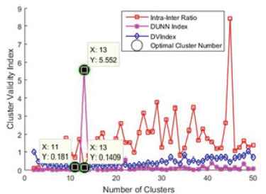
Positive class optimal cluster centers determination using three validity indices.
| -ve Class | +ve class | Total | |
|---|---|---|---|
| Intra-Inter Ratio Index | 30 | 13 | 43 |
| Dunn Index | 35 | 13 | 48 |
| Dynamic Validity Index | 13 | 11 | 24 |
Optimal number of clusters for each class using different validity indices.
From Fig. 5, we have observed that for negative class data intra-inter ratio index has obtained minimum value of 0.089 with 30 number of clusters, where as DV index obtained a minimum index value of 0.2346 with 13 clusters. Their corresponding cluster means are considered as optimal cluster centers. Unlike above two indices, we considered the maximum value for Dunn index and it is found that maximum value of 1.139 is obtained with 35 clusters. All these results are shown in Fig. 5. Similarly for positive class, optimal cluster centers have been obtained using three validity indices and these results are shown in Fig. 6.
The results from Fig. 5 and Fig. 6 are summarized in terms of optimal cluster number for each class using three validity indices. These summarized results are shown in Table 4.
Computational times for (finding cluster centers) proposed model and direct approach using three validity indices have been calculated and shown in Table 5. These results show that proposed model outperforms in terms of computational time as compared to direct approach.
| Index | Computational time using proposed model | Computational time using direct approach (Secs) | ||
|---|---|---|---|---|
| -Ve class data (Secs) | +Ve class data (Secs) | Total time (Secs) | ||
| Ratio | 1.47 | 1.34 | 2.81 | 8.21 |
| Dunn | 56.08 | 19.07 | 75.15 | 522.08 |
| DV | 1.58 | 1.01 | 2.59 | 9.36 |
Comparison of computational times.
After obtaining the cluster regions from Fig. 5 and Fig. 6, each region mean (center) and standard deviation (spread) has been calculated. These calculated values provided as inputs to the gaussian radial basis functions in RBFN pattern layer. Along with these radial basis neurons in pattern layer, input layer neurons, summation and decision layer neurons are collectively used for the construction of proposed RBFN model. Initially this RBFN has no weights, in order to find the weights between pattern layer and summation layer, this constructed RBFN has undergone training process using training data sets of both the classes. During this training process, Bat Algorithm with proper tuning parameters (these parameter values listed in table 1) has been employed.
The trained RBFN (with weights) is tested using testing data set (negative and positive class test data sets are combined) in order to evaluate RBFN performance. For every test data, RBFN outputs corresponding predicted pattern. These target and predicted patterns are compared to generate confusion matrix by making use of definitions given in Table 6. This confusion matrix helped in calculating the classification accuracy, sensitivity and specificity of the model using Eq. (31) – Eq. (33). In Table 6, we have explained the definitions of different parameters involved in confusion matrix.
| Abbreviation | Meaning |
|---|---|
| TP | True Positive count represents the number of patients that the model classified to have diabetes among the patients detected with diabetes by a medical doctor |
| TN | True Negative count represents the number of patients that the model classified to be non-diabetic among the patients detected as non-diabetic by a medical doctor |
| FP | is the False Positive count represents the number of patients that the model classified to be non-diabetic among the patients detected with diabetes by a medical doctor |
| FN | FN is the False Negative count represents the number of patients that the model classified to be non-diabetic among the patients detected with diabetes by a medical doctor |
Confusion matrix parameters definition.
Performance of proposed model with ratio, Dunn and DV indices are given in Tables 7, 8 and 9 respectively in the form of confusion matrix. This summarized results of three validity indices are given in Table 10. Results in Table 10 show that Proposed Model (PM) with intra-inter ratio index with 43 clusters locations achieves best accuracy of 70.00% compared to other two indices.
| Predicted class | ||||
|---|---|---|---|---|
| +ve | − ve | Total | ||
| Actual class | +ve | TP = 116 | FP = 34 | 150 |
| −ve | FN = 35 | TN = 45 | 80 | |
| Total | 151 | 79 | 230 | |
Confusion matrix for the proposed model with interintra ratio index
| Predicted class | ||||
|---|---|---|---|---|
| +ve | − ve | Total | ||
| Actual class | +ve | TP = 91 | FP = 59 | 150 |
| −ve | FN = 12 | TN = 68 | 80 | |
| Total | 103 | 127 | 230 | |
Confusion matrix for the proposed model with Dunn index.
| Predicted class | ||||
|---|---|---|---|---|
| +ve | − ve | Total | ||
| Actual class | +ve | TP = 120 | FP = 30 | 150 |
| -ve | FN = 40 | TN = 40 | 80 | |
| Total | 160 | 70 | 230 | |
Confusion matrix for the proposed model with DV Index.
| Optimal No.of Clusters | Accuracy | |
|---|---|---|
| Intra-Inter Ratio Index | 43 | 70.00 % |
| Dunn Index | 48 | 69.13 % |
| Dynamic Validity Index | 24 | 69.56 % |
Performance comparison of three validity indices.
Proposed model with three validity indices have been compared with conventional RBFN, these results are provided in Table 11. It has been observed from values in Table 11 that proposed model using any validity index (indices used in this paper) achieved more accuracy than conventional RBFN and also reduces the complexity of network (in terms of number of connections in model) to 96.88%. This in turn reduced the training time to below one second and classification time (time for classifying single unknown pattern by model) to 0.01 seconds, which is very less compared to conventional RBFN classification time of 0.46 seconds. This helps in classification of the unknown patterns very quickly. In terms of accuracy, ratio index has outperformed and in terms of training time, classification time and network complexity, DV index has outperformed. We have also observed that, the proposed model using any index reduces network complexity, training time, classification time without compromising accuracy.
| Conventional RBFN | RBFN + RatioIndex | RBFN + DunnIndex | RBFN + DVIndex | |
|---|---|---|---|---|
| # Hidden Layer Neurons | 768 | 43 | 48 | 24 |
| # Links (Complexity of network) | 7680 | 430 | 480 | 240 |
| Accuracy (%) | 68.53 | 70.00 | 69.33 | 69.56 |
| % Reduction in network complexity | 0% | 94.40% | 93.75% | 96.88% |
| Classification time (seconds) | 0.46 | 0.03 | 0.03 | 0.01 |
| Training time (seconds) | 269.75 | 1.18 | 1.32 | 0.31 |
Performance comparison of proposed model with different validity indices.
Performance of proposed model on PID dataset has been compared with existing models namely Cascade Forward Networks (CFN), Time Delay Networks (TDN), Feed Forward Networks (FFN), Decision tree based models like GINI and Artificial Immune System (AIS). For comparison purpose accuracy, sensitivity and specificity parameters have been calculated using Eq. (31) to Eq. (33). All these comparison results are presented in the Table 12 and the same results are shown in Fig. 7 using graphical chart. Proposed model results are highlighted in the Table 12. From results in Table 12, we have observed that the proposed model achieves better accuracy, sensitivity and specificity compared to various models reported by M. Bozkurt et al.12.
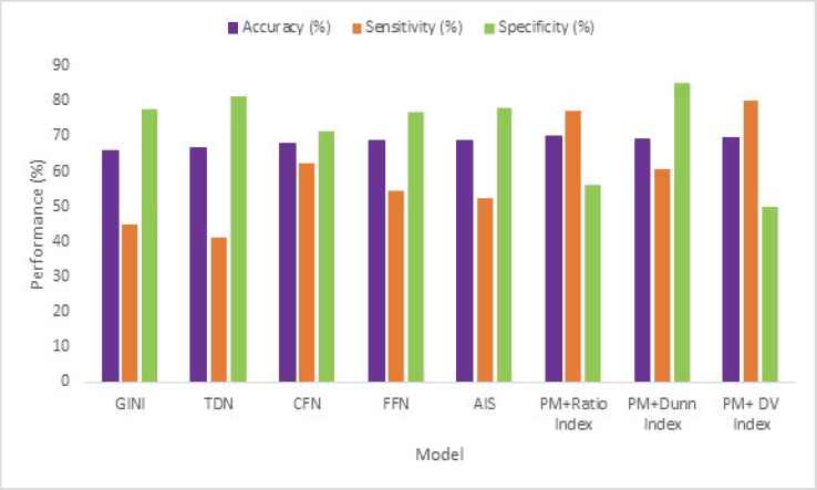
Graphical illustration of results for various models.
| Model | Dataset | Accuracy (%) | Sensitivity (%) | Specificity (%) |
|---|---|---|---|---|
| GINI | PID | 65.97% | 44.71% | 77.78% |
| TDN | PID | 66.80% | 41.11% | 81.25% |
| CFN | PID | 68.00% | 62.22% | 71.25% |
| FFN | PID | 68.80% | 54.44% | 76.88% |
| AIS | PID | 68.80% | 52.22% | 78.13% |
| Proposed Model (PM) with Ratio Index | PID | 70.00% | 77.34% | 56.25% |
| Proposed Model (PM) with Dunn Index | PID | 69.13% | 60.67% | 85.00% |
| Proposed Model (PM) with DV Index | PID | 69.56% | 80.00% | 50.00% |
Comparison of proposed model with various models.
4.3.2. Performance analysis on synthetic data sets
This section discusses experimental evaluation of proposed model on various synthetic data sets. These synthetic data sets are created using method explained in section 4.3. Each data set is partitioned into training and testing data sets according methodology shown in Fig. 4. Synthetic data sets of sizes 1500, 3000, 6000 and 12000 have been created and the corresponding training data sets are fed into proposed model to obtain optimal cluster locations for each class. These simulated ouptputs are shown in Fig. 8 and corresponding results are given in Table 13. In table 13, we listed computational time required to obtain optimal clusters inside each class, using proposed model and direct approach. These values are listed according validity indices namely ratio, Dunn and DV for data sets 1500, 3000, 6000 and 12000 respectively. The obtained optimal number of clusters for each class is enclosed in Table 13 using parentheses besides computational time values. These results proved once again that, even with larger data sets, proposed model achieves significant reduction in computational time compared to direct approach.
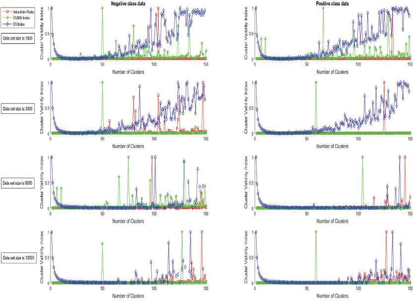
Optimal clusters determination using three validity indices for negative and positive class over synthetic data sets.
| Data set size | Validity Index | Computation time (Seconds) using proposed model for | Computation time (Seconds) using Direct Approach | Computational time reduction in (%) | ||
|---|---|---|---|---|---|---|
| −ve class | +ve class | Total Time | ||||
| 1500 | Ratio | 7.8 (37) | 7.25 (42) | 15.05 (79) | 34.86 | 56.82 |
| Dunn | 282.34 (50) | 282.65 (66) | 564.99 (116) | 2483.81 | 77.26 | |
| DV | 14.77 (27) | 14.25 (35) | 29.02 (62) | 105.65 | 72.53 | |
| 3000 | Ratio | 10 (46) | 7.99 (59) | 17.99 (105) | 48.83 | 63.15 |
| Dunn | 1772.82 (50) | 1547.70 (59) | 3320.52 (109) | 13166.94 | 74.79 | |
| DV | 20.95 (31) | 15.86 (25) | 36.81 (56) | 183.83 | 79.98 | |
| 6000 | Ratio | 10.34 (65) | 9.34 (72) | 19.68 (137) | 76.27 | 74.20 |
| Dunn | 3201.23 (74) | 2977.34 (107) | 6178. 57 (181) | 29093.39 | 78.76 | |
| DV | 10.55 (124) | 10.09 (142) | 20.64 (266) | 86.23 | 76.06 | |
| 12000 | Ratio | 20.16 (88) | 21.11 (74) | 41.27 (162) | 138.45 | 70.19 |
| Dunn | 4762.89 (126) | 5135.72 (113) | 9898.61 (239) | 54986.52 | 81.99 | |
| DV | 21.94 (114) | 21.89 (99) | 43.83 (243) | 144.75 | 69.72 | |
Proposed & direct approach performance over larger datasets.
From Table 13, we have observed that as data set size increases the number of optimal cluster locations of each class increases. Among the three validity indices the ratio index is simpler one and Dunn index is complicated one in terms of computation time. Further, the proposed model reduces the computation time drastically compared to direct approach.
To further evaluate the proposed model, we compared proposed model over conventional RBFN in terms of accuracy, complexity (number of connections or links), classification time (Time to classify single pattern) and training time (Time to obtain RBFN weights) by varying data set size from 1500 to 12000. These experimental results are given in Table 14 and these results show that proposed method works well on bigger data sets to achieve competitive accuracy, by reducing the network complexity, training time and classification time drastically.
| Data set size | Conventional RBFN | RBFN+ Ratio Index | RBFN+ Dunn Index | RBFN+ DV Index | |
|---|---|---|---|---|---|
| 1500 | # Hidden layer Neurons | 1050 | 79 | 116 | 62 |
| # Links | 10500 | 790 | 1160 | 620 | |
| Accuracy (%) | 71.34 | 72.23 | 71.77 | 72.46 | |
| % Reduction in network complexity | 0 | 92.47 | 88.95 | 94.09 | |
| Classification time (Seconds) | 0.61 | 0.03 | 0.061 | 0.024 | |
| Training time (Seconds) | 716 | 13.56 | 23.69 | 9.590 | |
| 3000 | # Hidden layer Neurons | 2100 | 105 | 109 | 56 |
| # Links | 21000 | 1050 | 1090 | 560 | |
| Accuracy (%) | 74.55 | 74.77 | 75.00 | 74.55 | |
| % Reduction in network complexity | 0 | 95 | 94.80 | 97.33 | |
| Classification time (Seconds) | 1.48 | 0.05 | 0.037 | 0.023 | |
| Training time (Seconds) | 3012.43 | 20.04 | 21.70 | 8.16 | |
| 6000 | # Hidden layer Neurons | 4200 | 131 | 181 | 236 |
| # Links | 42000 | 1310 | 1810 | 2360 | |
| Accuracy (%) | 71.42 | 71.45 | 71.57 | 71.66 | |
| % Reduction in network complexity | 0 | 96.88 | 95.69 | 94.38 | |
| Classification time (Seconds) | 13.47 | 0.038 | 0.051 | 0.072 | |
| Training time (Seconds) | 12122.54 | 27.38 | 41.59 | 57.00 | |
| 12000 | # Hidden layer Neurons | 8400 | 162 | 239 | 243 |
| # Links | 84000 | 1620 | 2390 | 2430 | |
| Accuracy (%) | 71.42 | 71.44 | 71.45 | 71.61 | |
| % Reduction in network complexity | 0 | 98.07 | 97.15 | 97.10 | |
| Classification time (Seconds) | 23.00 | 0.047 | 0.089 | 0.068 | |
| Training time (Seconds) | 23825.63 | 36.61 | 57.64 | 58.68 | |
Proposed model performance over larger data sets.
5. Conclusion
In this paper, a new model has been proposed for the classification of diabetic patients data. This proposed model comprises of construction and evaluation phases. In the construction phase, proposed model used integrated k-means in class by class fashion. This reduced the computational time for determining clusters without compromising the accuracy of the model. In evaluation phase, performance of model has been evaluatted with various performance measures such as accuracy, sensitivity, specificity, complexity, computational time, training time and classification time.
Experimental results on PID data set proved that proposed model with all three cluster validity indices with few neurons in pattern layer outperformed in terms of accuracy compared to PNN, FFN, CFN, TDN, GINI, AIS and conventional RBFN. Proposed model reduced not only the complexity of network by 96.88%, but also training time to below one second and classification time to 0.01 seconds.
Experimental results on synthetic data sets proved that proposed model with all three cluster validity indices reduced the computational time for determining the clusters drastically. Few neurons in pattern layer reduced the network complexity, training time and classification time. This proposed model also provided competitive accuracy compared to conventional RBFN.
Finally, by observing all the results we conclude that proposed model achieved competitive accuracy, by reducing the network complexity, training time and classification time drastically. This helps to create simple and powerful RBFN for the purpose of classification task.
References
Cite this article
TY  - JOUR
AU  - Ramalingaswamy Cheruku
AU  - Damodar Reddy Edla
AU  - Venkatanareshbabu Kuppili
PY  - 2017
DA  - 2017/01/01
TI  - Diabetes Classification using Radial Basis Function Network by Combining Cluster Validity Index and BAT Optimization with Novel Fitness Function
JO  - International Journal of Computational Intelligence Systems
SP  - 247
EP  - 265
VL  - 10
IS  - 1
SN  - 1875-6883
UR  - https://doi.org/10.2991/ijcis.2017.10.1.17
DO  - 10.2991/ijcis.2017.10.1.17
ID  - Cheruku2017
ER  -