
A new enhanced support vector model based on general variable neighborhood search algorithm for supplier performance evaluation: A case study
- DOI
- 10.2991/ijcis.2017.10.1.20How to use a DOI?
- Keywords
- Computational intelligence; Least square-support vector machine (LS-SVM); Supplier selection; Supplier Evaluation; Continuous general variable neighborhood search (CGVNS); Cosmetics industry
- Abstract
In sustainable supply chain networks, companies are obligated to have a systematic decision support system in place to help it adopt right decisions at right times. Among strategic decisions, supplier selection and evaluation outranks other decisions in terms of importance due to its long-term impacts. Besides, the adoption of such strategic decision entails exploring several factors that contribute to the complexity of decision making in the supply chain. For the purpose of solving non-linear regression problems, a novel neural network technique known as least square-support vector machine (LS-SVM) with maximum generalization ability has successfully been implemented. However, the performance quality of the LS-SVM is recognized to notoriously vary depending on the rigorous selection of its parameters. Therefore, in this paper, a continuous general variable neighborhood search (CGVNS) which is an effective meta-heuristic algorithm to solve the real world engineering continuous optimization problems is proposed to be integrated with LS-SVM. The CGVNS is hybridized in our novel integrated LS-SVM and CGVNS model, to tune the parameters of the LS-SVM to better estimate performance rating of supplier selection and evaluation problem. To demonstrate the improved performance of our proposed integrated model, a real data set from a case study of a supplier selection and evaluation problem is presented in a cosmetics industry. Additionally, comparative evaluations between our proposed model and the conventional techniques, namely nonlinear regression, multi-layer perceptron (MLP) neural network and LS-SVM is provided. The experimental results simply manifest the outperformance of our proposed model in terms of estimation accuracy and effective prediction.
- Copyright
- © 2017, the Authors. Published by Atlantis Press.
- Open Access
- This is an open access article under the CC BY-NC license (http://creativecommons.org/licences/by-nc/4.0/).
1. Introduction
Pressed with today’s global marketplace characterized by globalization, flourishing customers’ expectations, expanding regulatory conformity, global economic recession, and fierce competitive pressure, manufacturers cannot take on a life of their own. This simply implies that for manufacturers to outcompete their peers, they need to coalesce with their upstream and downstream partners. In fact, manufacturing firms must select and maintain core suppliers to ensure their survival and out-competition. Therefore, it goes without saying that rigorous supplier selection and evaluation constitutes a standout amongst the most impressive elements of purchase and supply management roles 1–3.
Many companies do not acquire any decision-making mechanism for the selection of their suppliers. They are partly right since supplier selection and evaluation is a mind-boggling and urgent procedure as a consequence of possibly conflicting multi-criteria, contribution of numerous choices and internal and external requirements dictated for buying process which might be conceived unsolvable with software 4.
AI-based models are recognized to be the best methods for selecting and evaluating the suppliers in the supply chain. Computer-aided decision making is possible taking into account purchasing experts and/or historic data. The neural network-based models, due to their merits are commonly-used among the existing techniques in the AI approach. Not requiring the complex process of the decision making is one of the main merits of the AI models. In the AI systems the client respects the information on the features of current situation (e.g., performance of a supplier versus the factor or criteria). Consequently, the AI technologies find the actual trade-off of the users according to learning from the supply chain experts or applications in the past. The technologies based on the AI also have been employed in domains of supplier 5–7.
Among AI models, support vector machine (SVM) introduced by Vapnik 8 has actually demonstrated it prospects in wide range of applications with stupendous results. The SVM is a novel neural network and supervised learning technique to tackle various regression problems. SVMs, due to their excellent performance in generalization and their capacity for self-learning, have overcome the potential weaknesses of conventional prediction techniques, namely artificial neural networks (ANNs) and fuzzy systems in real-world applications 9. Additionally, SVM ensures finding optimal solution as it utilizes a convex quadratic programming. Numerous industrial fields have benefited from implementing the SVM. For instance prediction of bankruptcy 10, forecasting tourism demand 11, time estimation in new product development projects12, cost estimation of the wing-box structural design 13, forecasting conceptual cost in construction projects 14 and supplier selection problem 15,16. However, similar to other AI algorithms, SVM model enjoys certain strengths and suffer from certain weaknesses. The obvious weakness of SVM is the selection of its parameters. Proper selection of SVM parameters significantly streamlines the accuracy of the prediction. Regretfully, SVM model suffers from lacking a systematic approach to calibrate its parameters. Several researchers have hybridized evolutionary algorithms as enhanced tools with SVM model to remedy this notorious deficiency. For example, Hong 17 proposed a SVR model with an Immune algorithm to forecast the electric loads. Huang18 presented a hybrid ant colony optimization (ACO)-based classifier model that combines ACO and SVM to improve classification accuracy with a small and appropriate feature subset. Wu 19 proposed a forecasting model based on chaotic SVM and genetic algorithm to consider demand series, providing good estimating and forecasting results of the product sale series. Cheng et al. 20 developed learning model fused two approaches of artificial intelligence, namely the fast messy genetic algorithm and SVM, to create a model of the evolutionary support vector machine inference. Wu21 presented a hybrid intelligent system for demand forecasting by combining the wavelet kernel support vector machine and particle swarm optimization.
Continuous general variable neighborhood search (CGVNS) introduced by Mladenović et al. 22 is a top-notch methodology capable of solving different types of continuous optimization which has been introduced in the recent years. The notable advantage of CGVNS as opposed to most local search-based heuristics is the utilization of solely one neighborhood search structure in that it systematically changes pre-specified neighborhoods within a local search strategy and owns fewer parameters to adjust. Hence, in this paper an attempt is made to streamline the performance rating of supplier in supplier selection and evaluation problem by introducing a novel hybrid meta-heuristic support vector model. The selection of parameters in the LS-SVM model is optimized by employing the CGVNS simultaneously. The proposed model is validated by using a real data set gathered from a case study for supplier selection and evaluation problem in a cosmetics industry. Comparative analyses are also conducted to appraise the performance of the proposed model and conventional techniques, including nonlinear regression, MLP neural network and LS-SVM. To the best of the authors’ knowledge, no hybrid CGVNS and SVM is found in the literature exploring the estimation and prediction problems.
The rest of this paper is structured as follows. The relevant literature review is presented and reviewed in section 2. Section 3 specifies criteria and construct hierarchical structure for supplier selection and evaluation problem in cosmetics industry. In Sections 4 and 5, some basic concepts on the LS-SVM and the CGVNS are succinctly given, respectively. In Section 6, the proposed LS-SVM model-based CGVNS is described for estimating the performance rating of supplier in supplier selection and evaluation problem. In Section 7, the comparisons among four artificial intelligence techniques are made. Finally, conclusion remarks are drawn in Section 8.
2. Literature review
As various quantitative methods regarding supplier selection and evaluation abound in the literature, they can be assigned to of the seven categories that we subsequently elaborate. A comprehensive review of the methods in the literature is proposed by Ho et al. 23.
2.1. Mathematical programming model
Ghodsypour and O’Brien 24 proposed a mixed integer non-linear programming approach to tackle the multi-criteria sourcing problem. The model is to find the optimal allocation of products to suppliers so that the total annual purchasing cost is minimized. Three constraints are incorporated in the model. A mixed-integer linear programming model for a problem of the supplier selection was extended by Hong et al. 25. The aim is to determine the optimal number of suppliers and the optimal order quantity so that the revenue is maximized. Wadhwa and Ravindran 26 studied the supplier selection problem (a multi-objective programming) by providing there three objective functions, such as minimization of price, lead time, and rejects were considered. A weighted linear programming model for a problem of the supplier selection was proposed by Ng 27 for maximizing the supplier score.
2.2. Multi-attributes decision making method
Vahdani et al. 28 provided a compromise solution method for solving fuzzy group decision-making problem by taking both conflicting quantitative and qualitative factors into account. Mousavi et al. 29 developed a multi-stage decision framework with interval-valued fuzzy sets to solve the decision problems under uncertain conditions. Vahdani et al. 30 focused on a hierarchical MCDM method with fuzzy-sets theory to handle the fuel buses selection problem.
2.3. Fuzzy sets theory
Vahdani et al. 31 introduced a mixed nonlinear facility location–allocation model for recycling collection centers. Vahdani et al. 32 designed a bi-objective model under uncertainty by regarding a reliable network of bi-directional facilities in logistics network. A fuzzy balancing and ranking method for the supplier selection problem was extended by Vahdani and Zandieh 33. This model consists of a four-stage algorithm to obtain the alternative outranking.
2.4. Intelligence approaches
The addressed artificial intelligence (AI) research in the area of supplier selection and evaluation can generally be introduced into two basic group:
- •
Artificial neural networks (ANNs)
- •
Fuzzy neural networks (FNNs)
A hybrid ANN and CBR approach to choose the most suitable and best supplier in the area of crisp neural networks was proposed by Choy et al. 34–35. ANNs are mostly employed to benchmark the potential suppliers, whereas CBR are employed to select the best supplier by considering the past fruitful and applicable cases. An ANN-based predictive model for forecasting the supplier’s bid prices in the process of supplier evaluation negotiation was developed by Lee and Yang36. Lau et al. 37 presented a hybrid ANN and GA approach for supplier selection. In their research, they utilize the ANN for benchmarking the potential suppliers or candidates with respect to evaluating factors or criteria and after that; the GA is used to find out the best combination of suppliers. An integrated NN-DEA for evaluation of suppliers under incomplete information of evaluation criteria was presented by Celebi and Bayraktar 38. Kuo et al. 15 developed an integrated ANN, DEA and ANP for a green supplier selection. This method considers practicality both in traditional supplier selection criteria and environmental regulations.
To assess supplier performance, Wu 39 proposed a hybrid model using DEA, decision trees (DT) and NNs. The model is composed of two elements: element 1 employs DEA and divides suppliers based on the resulting efficiency scores into two clusters: efficient and inefficient. Element 2 takes advantage of firm performance-related data to train DT, NNs model and apply the designed model of trained decision tree to new suppliers. Guo et al. 40 introduced potential support vector machine. Then, they combined it with decision tree to deal with issues on supplier selection including feature selection and multi-class classification. To harness the information-processing difficulties inherent in screening a large number of potential candidates or suppliers in the early phases of the selection process, a model is proposed by Luo et al. 41. By virtue of RBFANN, the model makes possible potential suppliers to be assessed by concurrently considering multiple evaluation attributes by quantitative and qualitative measures. Kuo et al. 16 in the area of fuzzy neural networks, designed an intelligent supplier decision support system capable of considering both the quantitative and qualitative factors.
2.5. Statistical/probabilistic approaches
A simulation-based approach considering uncertainty with respect to the demand for the item or service purchased was proposed by Soukoup 42. A cluster analysis approach for supplier evaluation problem was developed by Hinkle et al. 43.
2.6. Hybrid approaches
Vahdani et al. 44 developed an effective AI approach to enhance the decision making for a supply chain for long-term prediction in cosmetics industry. Vahdani et al. 45 extended a hybrid meta-heuristic algorithm for vehicle routing scheduling in cross-docking systems. Vahdani et al. 46 designed a bi-objective mixed integer linear programming model with multi-echelon, multi-facility, multi-product and multi-supplier and applied to a case study in iron and steel industry.
2.7. Other exciting methods
The supplier positioning matrix, modified from the product-process change matrix was suggested by Chou et al. 47 to link the capability of suppliers with the requirements of the customers to take the strategy-aligned factor or criteria into account for the vendor selection in a modified re-buy situation. Sevkli et al. 48 stated that the DEAHP method outperformed the AHP method for supplier selection.
Above, we have investigated seven categories of methods for solving supplier selection problem. Certain specific merits have been recognized for each category, although there might be some notorious shortcoming for each.
- •
MADM methods are very simple, but they depend tremendously on human judgments. For example, different attributes can take on different weights based on the decision-makers’ subjective judgment.
- •
Due to the quantitative nature of mathematical programming approaches, they create significant problems while taking into account qualitative factors. Moreover, in as much as these methods require arbitrary aspiration levels and they cannot accommodate subjective attributes.
- •
Fuzzy sets theory permits simultaneous consideration of precise and imprecise variables. On the other hand, owing to the complex nature of fuzzy set theory, it would be difficult for the users to grab the rationale for the output results.
Most of other categories fail to capture the interactions among the various factors and also cannot effectively consider risk in assessing the supplier’s execution and performance under uncertain conditions. AI approaches play significant role in this domain amongst the above methods. One of the notable features of this method as opposed to the other methods is that they do not entail defining the process of decision making. Moreover, AI technologies strike the concrete trade-off for the client based on what it has been assimilated from the expert experience or past cases. Regarding the ability and sufficiency of AI approaches, they can more effectively deal with complexity and vagueness inherent in decision-making than conventional methods.
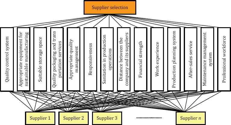
3. Criteria for supplier selection and evaluation in cosmetics industry
In this section, the definition of the criteria and constructing the hieratical structures are presented for supplier selection and evaluation problem in cosmetics industry. The goals of our hierarchy models are selecting and evaluating the supplier for the cosmetics industry that are identified in the first level in each hieratical structure. The second level in hieratical structure for selection supplier contains fourteen criteria, which are listed as follows:
- •
Quality control system (C1)
- •
Appropriate equipment for sustainable manufacturing (C2)
- •
Suitable storage space (C3)
- •
Packaging quality and transportation services (C4)
- •
Appropriate quality management (C5)
- •
Responsiveness (C6)
- •
Sanitation in production operations (C7)
- •
Distance between the company and its suppliers (C8)
- •
Financial strength (C9)
- •
Work experience (C10)
- •
Production planning system (C11)
- •
After-sales service (C12)
- •
Maintenance management system (C13)
- •
Professional workforce (C14)
The hierarchical structure for supplier selection presented in Fig. 1 shows the aforementioned criteria.
- •
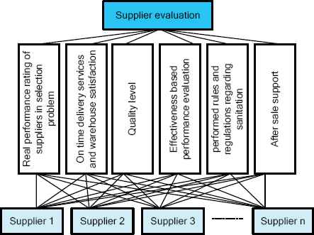
The second level in hieratical structure for evaluation supplier contains six criteria which are listed as follows:
- •
Real performance rating of suppliers in selection problem (phase 1)
- •
On time delivery services and warehouse satisfaction
- •
Quality level
- •
Effectiveness based performance evaluation for supplies and materials in production lines and afterwards
- •
Performed rules and regulations regarding sanitation
- •
After sale support
Hierarchical structure of the supplier selection problem in phase 1.
4. Least square-support vector machine (LS-SVM)
The LS-SVM is an extension of the SVM. Idea of the LS-SVM theory depends on mapping nonlinearly the original data in to a higher dimensional feature space 49. The assumption is that the data set S = {(x1, y1), … , (xn, yn)}, which processes a decision function and nonlinear function, can be written as illustrated in Eq. (1) 13, 49. In this equation, w denotes the weight vector; Φ represents the nonlinear function that maps the input space to a high-dimension feature space that provides linear regression, and b is the bias term 13, 49.
For the function estimation problem, the LS-SVM principle is provided and the optimization problem is utilized to formulate J function (2), where C denotes the regularization constant and ei represents the training data error.
Hierarchical structure of the supplier evaluation problem in phase 2.
To solve the above problem, the Lagrange multiplier optimal programming technique is applied to this constrained optimization problem. The technique considers objective and constraint terms concurrently. The Lagrange function L is illustrated as Eq. (4) 13, 49, 50.
In Eq. (4), αi ≥ 0 is named Lagrange multipliers, which can be either positive or negative due to the following equality constraints by regarding Karush–Kuhn–Tucher’s (KKT) conditions that present the extreme value in the saddle point; the conditions for optimality are introduced by Eqs. (5) to (8). This formula can be expressed as the solution to the following set of linear equations 49, 51.
In Eq. (9), Z = [Φ(x1)T;…;Φ(xn)T], y = [y1; …; yn], 1v = [1; …; 1], α = [α1; …; αn], and e = [e1; …; en]. The solution is provided by:
In order to simplify the solving process, let Ω = ZZT + C−1 I, where α and b are the solution to Eqs. (11) and (12):
The resulting LS-SVM model for function estimation is represented by:
In Eq. (13), the dot product k(x. xi) is known as the kernel function. Kernel functions empower the dot product to be computed and considered in a high-dimension feature space by using low-dimension space data input without the transfer function Φ and should satisfy the condition specified by Mercer 8,13. Commonly used kernel functions are given as follows.
- •
Linear function:
- •
Polynomial function:
- •
Radial basis function:
- •
Sigmoid function:
In the above equations, T, d, θ and γ denote the kernel function parameters 13, 51.
In concisely, major characteristics of the LS-SVM are presented as follows 11:
- •
The technique is capable to model nonlinear relationships.
- •
The training process in the LS-SVM can properly solve constrained quadratic programming problems linearly, and the LS-SVM inserted arrangement importance is remarkable, optimal and unlikely to generate local minima.
The technique picks just the important information points to consider and solve the regression function that presents the sparseness of a solution.
5. Continuous general variable neighborhood search (CGVNS) meta-heuristic
Mladenović and Hansen 52 first proposed VNS, a meta-heuristic technique which has quickly obtained massive success. Numerous papers have attempted to enhance and optimize their solutions by virtue of a relatively large arsenal of local search improvement heuristics, based around different neighborhood structures. The term variable neighborhood search refers to all local search-based algorithms systematically regarding the neighborhood structure during the search.
VNS has manifested its successful application to other problems including 53–55. The rationale behind the employment of VNS is that meta-heuristic algorithms get trapped in local optima. Such phenomenon occurs because of the myopic behavior of meta-heuristic algorithms: operator is unable to diversify the search space and stays focused around searching the current solution. Instead of relying on advanced meta-heuristics mechanisms such as random perturbations (iterated local search), memory structures (taboo search) or crossover and mutation in evolutionary methods, the VNS operates taking advantage of different types of neighborhoods, which might contain the required improving moves.
The mechanism of VNS is very much similar to that of Iterated Local Search (ILS). The VNS instead of iterating over one fixed type of neighborhood search structure (i.e. local search) as done in ILS, iterates in an appropriate way by considering some neighborhood structures until some stopping criterion is satisfied. The core procedures of the VNS are as below:
- (1)
A local minimum one-neighborhood structure is not as a matter of course locally negligible regarding another neighborhood structure.
- (2)
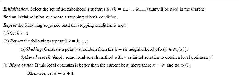
Steps of the basic VNS.
Mladenović et al. 56 for the first time presented the rules of VNS for solving a ‘‘pure’’ continuous mathematical-modeling problem. A poly-phase radar code design, the unconstrained non-linear problem that has specific minimax objective function is considered in their work. Mladenović el al. 57 and Kovacevic-Vujcić et al. 58 develop the software package global optimization for general box-constrained nonlinear programs. For the local search phase of VNS, several non-linear programming tools and methods, such as steepest descent, Rosenbrock, Nelder-Mead, Fletcher-Reeves, are included in our study. The proper specification as to what methods to be used is delegated to the user. In the shaking step, for defining neighborhoods in Rn, we make use of rectangular norm.
For solving box-constrained continuous global optimization problems, the advanced version of global optimization is suggested in 59. Therefore, for the shaking step, Mladenović et al. 22 consider several basic VNS heuristics, each using different metric function in designing neighborhoods. Users have full freedom to choose any combination of those heuristics. For each heuristic (metric) we perform the search with kmax (a VNS parameter) neighborhoods. In each of neighborhoods, according to the chosen metric, a random starting point for a local search is generated. Moreover, for finding three dimensional structure of the molecule, that is shown to be an unconstrained NLP problem in 60, Mladenović et al. 22 observed that the uniform distribution for generating points at random in the shaking step does not require the best choice 61; the specially designed distribution lets to get more initial solutions for descents nearer to axial directions and much better results in terms of computational efforts. A new heuristic for solving complex unconstrained continuous optimization and decision problems is developed by Mladenović et al. 22. The proposed heuristic is based on a generalized version of the variable neighborhood search meta-heuristic. Moreover, they develop VNS for tackling constrained optimization problems.
As opposed to discrete optimization, solution space and neighborhoods Nk(x) are infinite sets in continuous optimization. Hence, one cannot expect to completely provide any slight neighborhood of a point in a local search, which can be regarded as conventional in discrete case. However, we can utilize some local minimization algorithm from initial point. Local minimum attained by this minimizer can be far away from the initial point which we find to be a feature of the method because we are most of the time searching for a superior solution lying in several distant part of a solution space.
The neighborhoods Nk(x) denotes the set of solutions regarding the kth neighborhood of x, and using the metric ρk, it is defined as 22:
Where rk is the radius of Nk(x) monotonically non-decreasing with k. Notice that the same value of the radius can be utilized in some successive iterations. In other words, each neighborhood structure Nk is definedby pair (ρk, rk), k = 1,2, … , kmax. Basic steps of CGVNS meta-heuristic are given in Fig. 4 22.
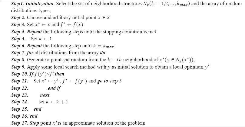
Pseudo-code of CGVNS.
The metric functions are defined in a usual way, i.e., as lp distance:
The CGVNS is a robust metaheuristic algorithm as it does not have any parameters needing to be tuned. Influential parameters are recognized as follows by Mladenović et al. 22 and Dražić et al. 61:
- •
Maximum allotted running time tmax for the search.
- •
Number of neighborhood structures kmax considered and used in the search;
- •
Values of radii rk; k = 1,2, … , kmax. Those values may be specified by user or computed automatically during the search.
- •
Geometry of neighborhood structures Nk, defined by the select of metrics ρk(x, y). Typical selections are l1, l2 and l∞.
- •
Type of statistical distribution which is utilized for obtaining the random point y from Nk in shaking step. Uniform distribution in Nk is the most straightforward choice, but employing other distributions may culminate in much better performance on some engineering and management problems.
- •
Local optimizer used in local search step. Usually the choice of the local optimizer is determined by the properties of the objective function. Numerous local optimization algorithms and methods are available both for smooth and non-differentiable functions.
- •
Requesting of neighborhoods and circulations in the shaking step.
6. Proposed support vector optimization model
The generalization ability and suitability along with predictive accuracy of the LS-SVM are dictated by searched problem parameters, comprised of independent parameters (i.e., parameter C and γ). As a matter of fact, the accuracy of model results is directly dictated by these selections. As far as we are concerned, the existing software does not possess a built-in mechanism to automatically calibrate parameters of the LS-SVM efficiently. Additionally, most researchers perform the trial-and-error procedure for the sake of parameters selection. To obtain optimal parameters, few LS-SVM models are constructed based on different parameter sets, then they are examined on a validation set. However, this procedure requires some luck and often is time-consuming 11.
To remedy the above-mentioned deficiencies, a novel support vector model is proposed in this paper for the supply chain. The model consists of two novel powerful approaches (i.e., LS-SVM and CGVNS). (1) The LS-SVM plays the role of a supervised learning tool to consider input–output mapping in the supply chain and to concentrate on performance rating of suppliers in supplier selection and evaluation problem. The CGVNS is employed to dynamically optimize the LS-SVM parameters in order to boost the prediction efficiency.
The LS-SVM-CGVNS algorithm in our problem of the supply chain is described with subsequent steps:
Step 1: Scale data. The input data are normalized to ensure that diverse units of estimation are evacuated and all factors or attributes are defined in the same range [0,1] by:
After implementing this transformation, the effect of dimension is removed from all the variables.
Step 2: Prepare needed data. Training and test data sets are considered.
Step 3: Initialize parameters of CGVNS such as number of neighborhood structures, maximal running time, ordering of neighborhoods and distributions, range of kernel function and its parameters including (C, γ).
Step 4: Select randomly a kernel function from common examples of kernel functions such as polynomials, Gaussian radial base, and sigmoid. Generate a random set of C and γ in the given valuing ranges. Each selected kernel function and its parameters such as C and γ is considered as an individual of LS-SVM.
Step 5: Deploy the selected parameters and the obtained support vectors to represent a LS-SVM model. To test estimation ability of the LS-SVMs, the testing samples are used. Applicability of the model is measured by fitness as
where, pi andStep 6: If fitness is accepted then the training procedure of LS-SVM terminates and the best SVMs are determined. Otherwise, go to the step 7 and produce the new solution.
Step 7: Determine a set of neighborhood structures Nk(k = 1,2, … , kmax) and the array of random distributions types.
Step 8: Determine iterative neighborhood structure: k ← 1
Step 9: Repeat the following step until k = kmax.
Step 10: Shaking. Generate a point yat random from the k − th neighborhood of x*(y ∈ Nk(x*)).
Step 11: Local search. Deploy some local search algorithm or method with y as initial solution to determine and obtain a local optimum y′.
Step 12: Move or not. Compute the fitness function value of each solution. If this local optimum is better than the current solution, move there (x* ← y′) and go to the step 8. Otherwise, set k ← k + 1.
Step 13: Reshape. Optionally change the set of neighborhood structures Nk(k = 1,2, … , kmax) (geometry defined by metric) and random point distribution.
Step 14: Stop condition checking: if stopping criteria (maximal running time predefined or the error accuracy of the fitness function) are met, go to step 15. Otherwise, go to the step 10.
Step 15: Terminate the training procedure, output the best solution.
In Fig. 5, the flowchart of framework of this model is illustrated. This figure depicts the framework of the proposed LS-SVM-CGVNS model. The CGVNS algorithm is utilized to explore a better combination of the two parameters in LS-SVM model. The values of two parameters are updated when a new solution of CGVNS algorithm is generated. Afterwards, a forecasting process is implemented and a forecasting error is computed. Finally, if the stopping criterion is satisfied, then stop the algorithm and the latest solution is a best solution. This algorithm is employed to find a better combination of the LS-SVM parameters so that a smaller fitness function is attained during estimation iteration.
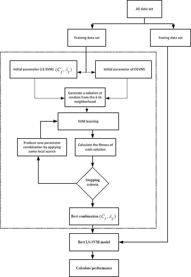
Framework of the proposed LS-SVM-CGVNS
7. Model validation and comparisons results
7.1. Data set
To test the effectiveness of the proposed model, we utilize a real set of performance rating of suppliers in cosmetics industry. Kaf Company is regarded as the leading producer of cosmetic and hygienic products in Iran and its oldest brand ‘DARUGAR’ is the first one of its kind in Iran. This company has always been identified as a pioneer of innovation and creativity in the industry in the last decade, and it still has successful presence in the market of Iran. Since this company produces more than many types of products, there is a major need to appraise the execution e rating of its potential candidates or suppliers.
On the other hand, problem of supplier evaluation and selection can be one of the most significant tasks and activities of purchasing management because of the key part of supplier’s performance on cost, quality, delivery and service in achieving objectives of the supply chain. In fact, supplier evaluation and selection for the company is regarded as a complex decision problem under uncertainty, affecting by different conflicting criteria. In order to implement the proposed LS-SVM-CGVNS, the above company is regarded as a real case study in cosmetics industry in this section.
The experimental data should be essential separated into the two subsets, namely the training data set and test data set. The data set size ought to be sufficient to give suitable training and test. A total of 55 training data points and 15 test data points are provided. Hence, the real data set is divided into training and test data set in the ratio of 75%: 25%. Table 1 illustrated 55 input data with respect to each criterion which are defined in section 3 for supplier selection problem and 15 validation cases. Furthermore, Table 2 demonstrates 55 input data with respect to each criterion, which are defined in section 3 for supplier evaluation problem and 15 validation cases.
| Input data | |||||||||||||||
|---|---|---|---|---|---|---|---|---|---|---|---|---|---|---|---|
| Suppliers | Criteria | Performance rating | |||||||||||||
| (C1) | (C2) | (C3) | (C4) | (C5) | (C6) | (C7) | (C8) | (C9) | (C10) | (C11) | (C12) | (C13) | (C14) | ||
| Score-Training data | |||||||||||||||
| s1 | 46 | 79 | 57 | 67 | 42 | 63 | 89 | 100 | 91 | 79 | 51 | 37 | 45 | 66 | 58.98 |
| s2 | 62 | 48 | 68 | 54 | 36 | 66 | 79 | 95 | 82 | 86 | 54 | 62 | 64 | 79 | 61.97 |
| s3 | 44 | 71 | 42 | 58 | 68 | 62 | 84 | 89 | 74 | 74 | 49 | 55 | 77 | 62 | 60.09 |
| s4 | 41 | 49 | 52 | 75 | 44 | 69 | 72 | 86 | 70 | 63 | 70 | 34 | 72 | 55 | 59.83 |
| s5 | 35 | 59 | 46 | 68 | 54 | 80 | 70 | 82 | 78 | 89 | 40 | 64 | 70 | 56 | 54.98 |
| s6 | 36 | 81 | 67 | 82 | 51 | 84 | 76 | 83 | 89 | 61 | 62 | 36 | 63 | 63 | 59.55 |
| s7 | 51 | 60 | 46 | 72 | 64 | 69 | 89 | 92 | 94 | 69 | 53 | 33 | 67 | 79 | 64.20 |
| s8 | 51 | 67 | 55 | 75 | 61 | 58 | 89 | 81 | 71 | 83 | 58 | 63 | 59 | 83 | 65.19 |
| s9 | 42 | 78 | 42 | 69 | 51 | 71 | 80 | 81 | 78 | 83 | 59 | 57 | 48 | 58 | 60.24 |
| s10 | 56 | 54 | 46 | 68 | 62 | 80 | 78 | 91 | 75 | 82 | 57 | 35 | 72 | 72 | 57.56 |
| s11 | 73 | 80 | 60 | 83 | 57 | 76 | 81 | 86 | 91 | 81 | 45 | 55 | 72 | 73 | 61.17 |
| s12 | 32 | 64 | 59 | 51 | 45 | 61 | 76 | 96 | 80 | 68 | 54 | 43 | 57 | 83 | 59.44 |
| s13 | 43 | 49 | 58 | 74 | 45 | 76 | 82 | 97 | 83 | 73 | 53 | 57 | 48 | 65 | 60.02 |
| s14 | 71 | 67 | 43 | 66 | 69 | 78 | 76 | 89 | 79 | 60 | 53 | 45 | 65 | 56 | 56.78 |
| s15 | 36 | 75 | 73 | 52 | 37 | 84 | 84 | 87 | 83 | 65 | 68 | 30 | 78 | 66 | 60.05 |
| s16 | 47 | 65 | 66 | 55 | 59 | 64 | 87 | 84 | 91 | 80 | 53 | 60 | 46 | 67 | 64.23 |
| s17 | 52 | 76 | 72 | 57 | 43 | 62 | 75 | 91 | 70 | 65 | 50 | 49 | 61 | 85 | 58.21 |
| s18 | 48 | 76 | 59 | 73 | 52 | 70 | 65 | 86 | 70 | 79 | 65 | 57 | 68 | 83 | 52.95 |
| s19 | 43 | 59 | 71 | 55 | 61 | 83 | 88 | 89 | 77 | 89 | 55 | 42 | 53 | 80 | 63.67 |
| s20 | 57 | 65 | 54 | 77 | 63 | 71 | 67 | 90 | 70 | 61 | 50 | 52 | 53 | 70 | 52.74 |
| ⋮ | ⋮ | ⋮ | ⋮ | ⋮ | ⋮ | ⋮ | ⋮ | ⋮ | ⋮ | ⋮ | ⋮ | ⋮ | ⋮ | ⋮ | ⋮ |
| s51 | 68 | 59 | 67 | 76 | 50 | 60 | 71 | 80 | 83 | 64 | 68 | 48 | 51 | 67 | 57.51 |
| s52 | 43 | 51 | 50 | 79 | 68 | 62 | 79 | 92 | 80 | 66 | 43 | 42 | 78 | 55 | 45.87 |
| s53 | 59 | 72 | 73 | 54 | 40 | 68 | 77 | 81 | 83 | 67 | 49 | 35 | 70 | 77 | 60.16 |
| s54 | 50 | 55 | 57 | 51 | 43 | 69 | 74 | 84 | 84 | 73 | 58 | 38 | 70 | 66 | 55.77 |
| s55 | 32 | 49 | 72 | 79 | 39 | 79 | 80 | 87 | 86 | 60 | 57 | 42 | 62 | 70 | 52.98 |
| Score-test data | |||||||||||||||
| s56 | 55 | 56 | 42 | 61 | 69 | 74 | 76 | 92 | 79 | 73 | 65 | 36 | 46 | 80 | 60.54 |
| s57 | 62 | 84 | 51 | 76 | 50 | 74 | 75 | 97 | 88 | 70 | 62 | 56 | 50 | 55 | 60.26 |
| s58 | 51 | 66 | 53 | 52 | 37 | 69 | 75 | 81 | 81 | 88 | 40 | 50 | 77 | 68 | 57.30 |
| s59 | 30 | 48 | 57 | 55 | 43 | 61 | 89 | 93 | 73 | 79 | 60 | 48 | 78 | 64 | 65.08 |
| s60 | 67 | 59 | 57 | 51 | 57 | 70 | 85 | 95 | 86 | 77 | 66 | 64 | 78 | 56 | 60.67 |
| s61 | 33 | 75 | 74 | 66 | 65 | 62 | 78 | 83 | 88 | 83 | 64 | 53 | 72 | 73 | 62.44 |
| s62 | 70 | 77 | 45 | 70 | 40 | 67 | 84 | 86 | 91 | 84 | 44 | 43 | 67 | 85 | 66.27 |
| s63 | 31 | 65 | 46 | 80 | 45 | 76 | 81 | 98 | 80 | 80 | 57 | 58 | 57 | 65 | 67.60 |
| s64 | 56 | 56 | 75 | 53 | 40 | 78 | 81 | 94 | 84 | 60 | 42 | 34 | 45 | 78 | 61.67 |
| s65 | 48 | 85 | 77 | 69 | 38 | 67 | 87 | 98 | 83 | 65 | 59 | 31 | 53 | 72 | 67.31 |
| s66 | 55 | 75 | 57 | 66 | 50 | 55 | 86 | 88 | 75 | 70 | 51 | 51 | 57 | 71 | 69.93 |
| s67 | 36 | 47 | 56 | 76 | 55 | 80 | 88 | 93 | 75 | 68 | 43 | 56 | 78 | 77 | 50.14 |
| s68 | 46 | 57 | 59 | 66 | 68 | 82 | 83 | 97 | 77 | 63 | 57 | 62 | 72 | 78 | 47.76 |
| s69 | 73 | 55 | 42 | 77 | 62 | 64 | 84 | 82 | 86 | 86 | 41 | 61 | 71 | 72 | 67.25 |
| s70 | 49 | 71 | 45 | 60 | 38 | 78 | 81 | 91 | 83 | 64 | 49 | 62 | 56 | 79 | 41.16 |
Patterns for conceptual predicting of performance rating of supplier in selection problem
| Suppliers | Input data | ||||||
|---|---|---|---|---|---|---|---|
| Criteria | Performance rating | ||||||
| (C1) | (C2) | (C3) | (C4) | (C5) | (C6) | ||
| Score-Training data | |||||||
| s1 | 58.98 | 46 | 40 | 53 | 69 | 33 | 48.55 |
| s2 | 61.97 | 68 | 54 | 49 | 74 | 36 | 56.02 |
| s3 | 60.09 | 46 | 62 | 58 | 71 | 53 | 65.34 |
| s4 | 59.83 | 68 | 69 | 57 | 75 | 50 | 64.06 |
| s5 | 54.98 | 46 | 70 | 57 | 56 | 30 | 50.13 |
| s6 | 59.55 | 50 | 57 | 53 | 57 | 48 | 60.87 |
| s7 | 64.20 | 73 | 41 | 37 | 71 | 53 | 65.60 |
| s8 | 65.19 | 75 | 57 | 42 | 58 | 53 | 64.22 |
| s9 | 60.24 | 59 | 60 | 45 | 57 | 42 | 57.47 |
| s10 | 57.56 | 69 | 56 | 57 | 61 | 30 | 50.86 |
| s11 | 61.17 | 71 | 49 | 41 | 76 | 38 | 57.35 |
| s12 | 59.44 | 72 | 59 | 60 | 64 | 32 | 52.46 |
| s13 | 60.02 | 49 | 69 | 41 | 74 | 45 | 61.07 |
| s14 | 56.78 | 49 | 44 | 55 | 57 | 31 | 50.93 |
| s15 | 60.05 | 65 | 55 | 54 | 73 | 32 | 53.50 |
| s16 | 64.23 | 52 | 47 | 44 | 55 | 31 | 51.16 |
| s17 | 58.21 | 69 | 67 | 55 | 74 | 42 | 59.25 |
| s18 | 52.95 | 65 | 44 | 45 | 79 | 31 | 53.15 |
| s19 | 63.67 | 69 | 66 | 47 | 60 | 51 | 63.19 |
| s20 | 52.74 | 59 | 45 | 40 | 65 | 37 | 55.02 |
| ⋮ | ⋮ | ⋮ | ⋮ | ⋮ | ⋮ | ⋮ | ⋮ |
| s51 | 57.51 | 68 | 50 | 57 | 68 | 37 | 55.66 |
| s52 | 45.87 | 72 | 56 | 47 | 66 | 50 | 62.19 |
| s53 | 60.16 | 59 | 65 | 58 | 78 | 43 | 60.38 |
| s54 | 55.77 | 46 | 51 | 54 | 69 | 48 | 61.97 |
| s55 | 52.98 | 72 | 47 | 56 | 57 | 48 | 60.48 |
| Score-test data | |||||||
| s56 | 60.54 | 58 | 40 | 56 | 79 | 45 | 61.66 |
| s57 | 60.26 | 53 | 61 | 38 | 65 | 49 | 62.38 |
| s58 | 57.30 | 46 | 68 | 49 | 61 | 50 | 62.33 |
| s59 | 65.08 | 54 | 45 | 41 | 75 | 36 | 56.32 |
| s60 | 60.67 | 70 | 50 | 43 | 72 | 52 | 64.92 |
| s61 | 62.44 | 65 | 57 | 41 | 66 | 51 | 63.78 |
| s62 | 66.27 | 60 | 55 | 59 | 72 | 45 | 61.24 |
| s63 | 67.60 | 57 | 53 | 48 | 69 | 37 | 56.38 |
| s64 | 61.67 | 45 | 61 | 41 | 68 | 39 | 57.05 |
| s65 | 67.31 | 70 | 61 | 56 | 60 | 51 | 63.42 |
| s66 | 69.93 | 60 | 51 | 54 | 64 | 37 | 55.97 |
| s67 | 50.14 | 52 | 57 | 53 | 58 | 50 | 61.56 |
| s68 | 47.76 | 74 | 68 | 38 | 56 | 44 | 57.75 |
| s69 | 67.25 | 63 | 53 | 57 | 75 | 53 | 66.23 |
| s70 | 41.16 | 46 | 51 | 52 | 60 | 31 | 50.30 |
Patterns for conceptual predicting of performance rating of supplier in evaluation problem
7.2. Performance criteria
Common statistical metrics including (1) mean absolute percentage error (MAPE), (2) root mean squared error(RMSE), (3) standard deviation error (SDE) and (4) R-squared (R2) are employed to evaluate the estimation performance of the proposed models. These metrics are defined by 13, 49–51, 62–66:
- (1)
- (2)
- (3)
- (4)where, pi and
The above-mentioned criteria are regarded as commonly-used measures for differences between values in statistics in the related literature, particularly in trend estimations 13, 49–51. The lower values of the first three criteria (i.e., MAPE, RMSE, SDE) indicate the better performance and more accuracy in the estimations in the supply chain. The fourth performance criterion (R2) is better when this criterion’s value is closer to 1. The explanations of these commonly-used performance criteria are presented as follows:
- •
The first performance criterion, MAPE, is regarded as a relative measure that represents errors as a percentage of the actual data. The main advantage of this criterion is that this performance measure in the supply chain introduces an easy and effective way of judging the extent or importance of errors for the estimations 13, 49.
- •
The second performance criterion, RMSE, denotes the deviation between the actual and estimated values by the proposed model; hence, smaller values of this criterion are preferred. The performance measure shows the sample standard deviation of the differences between estimated values and actual values, and integrates the magnitudes of the errors in estimations of the supply chain for different times into a single measure of predictive one 50, 51.
- •
- •
The fourth performance criterion, R2, expresses a number that includes the proportion of the deviation between the actual and predicted values in the dependent variable of the supply chain for the trend estimations, predictable from the independent variable. The aim of this performance criterion is the estimation of future trend outcomes and also testing of hypotheses for the forecasting 49–51.
In this paper, the radial basis function is employed as the kernel function for performance prediction in the supplier selection and evaluation. There are two independent parameters while using RBF kernels (i.e., C and γ). In fact, searching two parameters is highly important for the best estimation and forecasting ability. For this, the searching process of optimal parameters is operated with 100 generations in total. Finally, the parameters in our proposed model are as follows:
In supplier selection problem: C = 43740 and γ = 0.06 and in supplier evaluation problem C = 4980 and γ = 0.0003.
The processes of determining the parameters for three conventional techniques are presented. The first technique (i.e., MLP) is a feed forward ANN model that maps sets of input data onto a set of appropriate output67. This technique contains multiple layers of nodes in a directed graph, which is fully connected from one layer to the next. With the exception of the input nodes, each node is a neuron (or processing element) with a nonlinear activation function. The MLP uses a supervised learning technique called back propagation, for training the network 68. The designed MLP includes only one hidden layer for the application of the supplier selection and evaluation. Also, this paper considered and used a standard two-layer network. The input layer contains three nodes. The number of output nodes is set to 1. The number of neurons in the hidden layer is 6. The activation functions for the hidden and output layers are regarded as the hyperbolic tangent transfer function and linear function respectively. To train the network Levenberg-Marquardt back propagation is considered and used.
The second conventional technique (i.e., nonlinear regression) includes some function types. For simple estimation and forecasting problems, a one-order regression method is appropriate and suitable. However, with increasing the complexity of the variables and issue’ qualities, a nonlinear regression form are considered to solve different estimation and forecasting problems. The formula of the nonlinear regression is described by:
The third conventional technique (i.e., pure SVM) is a new machine learning based on the statistical learning theory, which has several advantages over the conventional ANN techniques. There are no general rules for setting the SVM parameters. The authors’ experience and trial-and-error are employed. Finally, the values of parameters obtained by the pure SVM technique are:
In supplier selection problem: C = 356000 and γ = 0.03 and in supplier evaluation problem C = 34000 and γ = 0.0002.
The overall comparative results based on the MAPE, RMSE, SDE and R2 indices are illustrated for the proposed models in Tables 3 and 4 (supplier selection and evaluation problem, respectively).
| Intelligent techniques | MAPE | RMSE | SDE | R2 |
|---|---|---|---|---|
| NLR | 12.5207 | 9.1445 | 0.1436 | -0.3282 |
| MLP | 11.2684 | 8.0594 | 0.0883 | -0.0317 |
| LS-SVM | 11.1041 | 8.2353 | 0.1399 | -0.0772 |
| LS-SVM-CGVNS | 10.7569 | 7.8095 | 0.1249 | 0.0313 |
Overall comparative results (selection problem)
| Intelligent techniques | MAPE | RMSE | SDE | R2 |
|---|---|---|---|---|
| NLR | 0.5016 | 0.3643 | 0.0037 | 0.9923 |
| MLP | 0.4241 | 0.2963 | 0.0026 | 0.9948 |
| LS-SVM | 0.3970 | 0.3145 | 0.0042 | 0.9942 |
| LS-SVM-CGVNS | 0.3172 | 0.2597 | 0.0035 | 0.9961 |
Overall comparative results (evaluation problem)
According to four commonly-used measures in the related literature reported in Tables 3 and 4, the computational results indicate that the proposed model has achieved lowest prediction error and highest forecasting ability in the supply chain. The proposed model is compared with other intelligent techniques, including NLR, MLP, and LS-SVM, for performance prediction in the supplier selection and evaluation. In fact, the proposed LS-SVM-CGVNS has lower values based on the first three performance criteria (MAPE, RMSE and SDE), and it also has higher value based on the fourth performance criterion (R2).
The results demonstrate the capability of the proposed model to produce lower error rates as compared to the three intelligent techniques for the selection problem in the supply chain management. For instance, the proposed LS-SVM-CGVNS model has recorded 10.7569 and 0.3172 of the first performance criterion, MAPE, for the first and second phases of the decision process in the supply chain, respectively, to quantify the deviation between the actual and predicted values. They denote lowest values among the results produced by four intelligent techniques in the supply chain management. Also, the proposed model has recorded 0.0313 and 0.9961 of the fourth performance criterion, R2, for the first and second phases of the decision process, respectively, to include the proportion of the deviation between the actual and predicted values for the supply chain’ trend estimations. They denote highest values among the results produced by four well-known intelligent techniques for the supplier selection and evaluation problem.
As can be seen from Tables 3 and 4, LS-SVM-CGVNS model is placed in the first rank, and models LS-SVM, MLP and NLR are placed in the second, third and fourth ranks, respectively in each problem. Moreover, Figs. 6 and 7 compare the results obtained with the prediction results from NLR, MLP, LS-SVM and LS-SVM-CGVNS with actual performance rating of suppliers for test records (56-70) respectively.
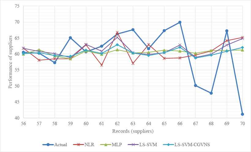
Comparison between actual performance ratings, NLR, MLP, LS-SVM and LS-SVM-CGVNS in supplier selection
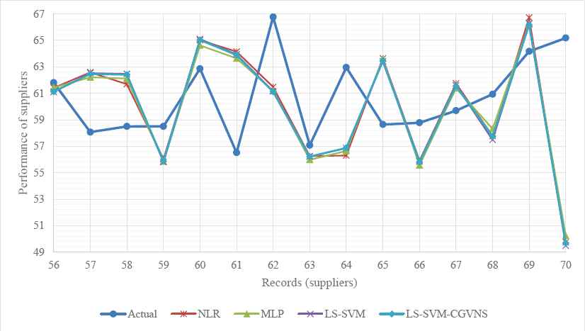
Comparison between actual performance ratings, NLR, MLP, LS-SVM and LS-SVM-CGVNS in supplier evaluation
The computational results provided by the three intelligent techniques, including NLR, MLP, and LS-SVM, and the proposed LS-SVM-CGVNS model are compared and depicted in Figs. 6 and 7 by considering actual and overall performances of suppliers for test records (56–70) for the supplier selection and evaluation. Fig. 6 depicts the performance ratings of the fifteen suppliers from the proposed intelligent model and three well-known techniques for the supplier selection problem in the phase 1 of the decision process in the supply chain management, compared with actual data. Then, Fig. 7 depicts the performance ratings of the suppliers for the supplier evaluation problem in the phase 2 of the decision process, compared with actual data from the proposed LS-SVM-CGVNS model and other intelligent techniques. It is figured out that the overall performance estimation of fifteen suppliers from the presented intelligent model are near to actual performance data.
Finally, a new intelligent model based on the LS-SVM with CGVNS has been proposed and implemented to predict the performance rating of the suppliers in the cosmetics industry, which had further focal points with attributes of higher reliability and avoid of over-fitting. The LS-SVM as a new ANNs has been taken into account with maximum generalization ability that has been implemented in many different management and engineering fields successfully. The selection of parameters in the LS-SVM model is optimized by utilizing the CGVNS simultaneously. The CGVNS as new algorithm is capable of solving different types of continuous optimization that have been applied to tune the parameters of the LS-SVM to better estimate performance rating of supplier selection and evaluation problem. It systematically changes pre-specified neighborhoods within a local search strategy and owns fewer parameters to adjust, and is capable to model nonlinear relationships in the cosmetics industry.
In sum, the advantages of the proposed hybrid intelligent model, in terms of all performance criteria regarding the forecasting accuracy, unlike the previous intelligent techniques, in the supply chain management are as follows:
- (1)
The LS-SVM-CGVNS model contain nonlinear mapping capabilities, and then can provide and capture data patterns of time intervals in the supply chain management more easily than multiple linear regression models;
- (2)
The LS-SVM-CGVNS model can minimize the structural risk instead of the training errors. The minimization of an upper bound on the generalization error results in higher generalization performance in the supply chain management unlike traditional forecasting techniques; and
- (3)
Since the choice of influential parameters in the LS-SVM model has remarkably impact on the prediction performance, unsuitable selection of these parameters results in either over-fitting or under-fitting of the LS-SVM. Therefore, the CGVNS algorithm is applied to solve this selection problem optimally in the supply chain management and to save the computational time properly.
The encouraging results obtained by the proposed LS-SVM-CGVNS model indicate a positive opportunity to be considered and to be utilized in the future for the supply chain decisions for the long-term, mid-term and short-term planning by introducing suitable prediction outcomes from the context of this paper.
8. Conclusions
Supplier selection and evaluation is affected by many factors whose effects are very complex to be identified by traditional methods. Hence, to overcome this problem, this work proposed a novel hybrid artificial intelligence model based on continuous general variable neighborhood search algorithm and least square-support vector machine. Support vector machine is presented and considered to build the non-linear relationship between selection, evaluation criteria and performance rating of suppliers and has demonstrated brilliant execution of non-linear representation based on little samples. Continuous general variable neighborhood search algorithm is used to improve the generalization performance in searching the support vector machine model, and has proved powerful global optimal performance. To demonstrate the effectiveness of the proposed model, we utilized real test data set in supplier selection and evaluation problems in the cosmetics industry and compared our model with three well-known techniques, including NLR, MLP and LS-SVM, for the performance rating estimation. Through comparison, it is concluded that the proposed model has a better generalization performance and yields lower estimation error. Performances the proposed model for performance rating prediction is affected by the value of the input parameter. As further research, the optimization of the proposed model is prescribed to enhance the computational expectation results.
References
Cite this article
TY  - JOUR
AU  - Behnam Vahdani
AU  - S. Meysam Mousavi
AU  - R. Tavakkoli-Moghaddam
AU  - H. Hashemi
PY  - 2017
DA  - 2017/01/01
TI  - A new enhanced support vector model based on general variable neighborhood search algorithm for supplier performance evaluation: A case study
JO  - International Journal of Computational Intelligence Systems
SP  - 293
EP  - 311
VL  - 10
IS  - 1
SN  - 1875-6883
UR  - https://doi.org/10.2991/ijcis.2017.10.1.20
DO  - 10.2991/ijcis.2017.10.1.20
ID  - Vahdani2017
ER  -