
A Performance Comparison of Neural Networks in Forecasting Stock Price Trend
- DOI
- 10.2991/ijcis.2017.10.1.23How to use a DOI?
- Keywords
- Stock market; BP neural network; Elman neural network; CSI 300 Index; relative error
- Abstract
The stock price shows the character of complex non-linear system, along with changes of internal and external environmental factors in stock market. As a form of artificial intelligence, neural network can fully reveal the complex relationship between investors and price fluctuations. After comparing network structures of different neural networks, the conclusions show Elman neural network has an obvious advantage over BP neural network in predicting price trend of Chinese stock market both in theory and practice.
- Copyright
- © 2017, the Authors. Published by Atlantis Press.
- Open Access
- This is an open access article under the CC BY-NC license (http://creativecommons.org/licences/by-nc/4.0/).
1. Introduction
Stock market can help capital demanders gain capitals and provide capital suppliers with investment tools. In order to forecast stock price trend, investors have to face various factors, coming from corporate operational performance and external environment. Many literature about prediction of stock price are easily found in the academic community. At present, the research methods of available literature mainly center on investment analysis method, time series analysis method, chaos theory method and artificial intelligence method.
Firstly, investment analysis method has two types: fundamental analysis and technical analysis. Fundamental analysis bases on the intrinsic value of stock, which is influenced by industry development, macroeconomic situation, fiscal policy, inflation, interest rate, corporate financial performance, and so on. Many financial problems can be further analyzed by fundamental analysis, such as institutional investment, arbitrage behavior, price trend forecasting and financial marketing strategy. Technical analysis based on the stock investment theories, focuses on the trend of price movement and the change of stock-trading volume. Although forecasting results may be accurate by adopting technical analysis in the short run, the long trend of market is not suitable for using technical analysis method, but rather fundamental analysis method. In the case of Chinese stock market, the results of technical analysis show stock price index can be predicted to a certain extent1. Many high frequency data of financial market can be applied to technical analysis in research areas of market efficiency2. As the relationship of fundamental analysis and technical analysis is complement rather substitute, the researches on stock price index gradually appear the integration trend of fundamental analysis and technical analysis3,4. In addition, the combinations of fundamental analysis and technical analysis are also used for analyzing other financial fields, such as foreign exchange market, financial performance and emerging currency markets5–7.
Secondly, time series analysis method mainly researches movements of data by using mathematical and statistic rules. Time series analysis includes statistical analysis, statistical modeling, optimistic prediction, filtering and control, and so forth. Based on financial time series, econometric models can make accurate analyses of stock price and help investors make optimal investment decisions. In many econometric models, GARCH model has been used widely in time series analysis. For example, Bonato in Ref. [8] introduced a multivariate stable-GARCH model in the process of studying tail characteristics of stock returns. Jammazi used wavelet-multivariate Markov switching GARCH approach to investigate the oil shock impact on stock market returns9. With the application of copula function in nonlinear systems, a copula approach analyzing tail dependence in different markets was put forward by Dajcman based on GARCH model10. Moreover, the development of fuzzy mathematics makes it possible to do some researches on financial market combining time series data. For examples, Huarng and Yu forecasted stock index with the help of a type 2 fuzzy time series model11. In the last few years, time series analysis combined with fractal method gradually has been applied to study stock trend. Yi et al. in Ref. [12] discussed the fractal characteristics of stock market using time times and validation of time series model. Chimanga and Mlambo in Ref. [13] focused on Johannesburg stock exchange indices and found a long term trend of all stock exchange indices by means of analyzing the fractal characteristic of time series.
Thirdly, chaos analysis method regards stock market as a chaotic system in which nonlinear methods can be used for studying fluctuation mechanisms of stock price. The forecasting method of chaos theory comprises local method, globe method, weighted local method, and so on. However, the existing literature usually adopts some improved chaos analysis methods by combining other research techniques to describe financial market. In Ref. [14], Chen used nonlinear theory and chaos analysis method to analyze financial market, and proposed a fractional-order financial system, which displayed investors’ trading characteristics such as fixed points and periodic motions. Nonlinear theory and chaos analysis method are also used in Cournot duopoly model. Wu et al. made a further study of complex nonlinear economic dynamics in Cournot duopoly model and showed the topological horseshoe chaotic characteristic by means of topological horseshoe theory15. In Ref. [16], Ozun et al. considered that chaos theory was well suited for examining the time series of stock index returns by profiling sample data of Greek stock market and Turkish stock market. In order to study chaos in German stock market, Webel found a strong evidence on chaos to returns by the approach of wavelet denoising and the 0-1 test17. In Ref. [18], Dobrescu et al. put forward a discrete-delay dynamic model with the aid of bifurcation analysis and chaos analysis. This model shows the evolution characteristic of a stock market price index. On the basis of ISE-100 data, chaos analysis method was used by Ozdemir and Akgul for exploring stock market structure in Ref. [19].
Fourthly, artificial intelligence method essentially is a simulacrum for thinking and consciousness of human brain. In consideration of complexity of financial market and nonlinear feature of financial variable, artificial neural network as an important form of artificial intelligence, has been a great development in many financial fields. Artificial neural network simulates the movement process of neurons cells of human brain. Specifically, artificial neural network is composed of a large number of neurons linking with each other and automatically change network structure by adjusting the weights of neurons in order to simulate samples data. Artificial neural network has great ability of data fitting and excellent characteristic, which can deal with complex problems. According to different structures of network, artificial neural network is divided into two parts: feedforward neural network and feedback neural network. In particular, input signals directly transmit from the former layer to the latter layer without feedback mechanism in feedforward neural network, such as BP neural network and RBP neural network. If feedback mechanism exists, it is called feedback neural network, such as Hopfield neural network and Elman neural network.
Many scholars used the combination method of neural network and other approaches to accurately describe feature of financial variable. Based on traditional RBF neural network, Akbilgic et al. in Ref. [20] introduced a novel HRBF neural network to reveal the relationship among different stock market indices in Istanbul stock exchange. According to evolutionary theory, Bisoi and Dash came up with a hybrid neural network having dynamic evolution characteristics in conjunction with unscented Kalman filter to forecast the change of stock price21. In Ref. [22], Sermpinis et al. applied stochastic neural network and genetic neural network to predict trade behavior of investors in financial market. In terms of research results got by Sermpinis et al., the Psi-Sigma network and SVR algorithm showed better performances about optimization of trading strategies. In addition, econometric models are also applied to neural networks, such as the combination between GARCH model and neural network. According to this line of thinking, Kristjanpoller et al. in Ref. [23] forecasted Brazil stock price index, Chile stock price index and Mexico stock price index by the use of a hybrid neural networks-GARCH model.
How many discrepancies can the different network structures produce in aspect of predicting stock price trend? In order to simplify this problem, BP neural network is chosen as a representative of feedforward neural network and Elman neural network is selected as a representative of feedback neural network in this paper. That is to say, BP neural network and Elman neural network are used to analyze the discrepancies of forecasting results. In section 2, the theories of BP neural network and Elman neural network are systematically described. Section 3 shows differential analyses between BP neural network and Elman neural networks based on the data in Chinese stock market. The conclusions are drawn in section 4 followed by references section.
2. A theoretical overview of neural network
Artificial neural network is composed of many neurons linking with each other. Every neuron indicates a signal output function, which is called activation function. And the linkage between two neurons can be described as signal weigh. Because linking mode, activation function and signal weight are probably different in dealing with complexities, the appropriate form of neural network need to be frequently adjusted in order to obtain a good fitting result. Artificial neural network has many excellent properties that contain self-learning, nonlinearity, rebustness, fault tolerance, parallel computation, and distribution storage. The character of self-learning is an ability that can change network performance to adapt a changing environment. In reality, economic system can be seen as a complex system, which is similar to the neural system of human brain. As a simulation of brain neurons, artificial neural network has nonlinear characteristics. Moreover, local damage and overload of the network never bring a deathblow to itself. Every neuron can independently and simultaneously deal with the information received in the same layer.
This section respectively introduces BP neural network and Elman neural network from a theoretical perspective. Through theoretical analysis, network structures and algorithms of two neural networks are shown and compared. The goal of comparative analysis is to get results between the performances differences of two neural networks in theory, and lay foundations for performance comparison in forecasting price trend of Chinese stock market.
2.1. The theory overview of BP neural network
BP neural network presented by Rumelhart and McCelland, is one of the most widely used neural networks in scientific researches24. BP neural network is also a kind of feedforward neural network trained by back propagation algorithm. In a basic BP neural network model, three network layers that compromise input layer, hidden layer and output layer, form the whole network structure. In Fig. 1, three network layers can easily be seen.

The structure of BP neural network
Above variables can be denoted by expression (1), (2) and (3). In expression (1), x indicates input vector containing M input values. In hidden layer, neurons are denoted by symbol K. From Fig. 1 and expression (2), it is easy to find out I neurons in hidden layer. Output vector indicates Y seen from expression (3), which is comprised of J output values in output layer. Signal weight can be written as ω connecting with neurons in different layers. Because of three layers in Fig. 1, signal weight can be divided into two types: ωmi and ωij. In particular, ωmi affects the signal transmission from input layer to hidden layer, and ωij affects the signal transmission from hidden layer to output layer. However, BP neural network may also have several hidden layers rather than only one hidden layer. But Kolmogorov theorem proven by Hecht-Nielsen in Ref. [25] shows that three layers structure of BP neural network can approximate any continuous function in a closed interval.
Let eBP be an error function of BP neural network, which is shown as follow.
Every layer of BP neural network has many neurons that have never contact each other. However, the only connection between neurons happens in different layers. Input signal transmits from input layer to hidden layer to output layer after a series of function transformation. If analytical results from output layer have large deviations with expected results, BP neural network will adjust weight values among of neurons by back propagation algorithm. This process of adjustments will end up once analytical results are satisfied with error precision. The entire running process of BP neural network can be shown in Fig. 2.
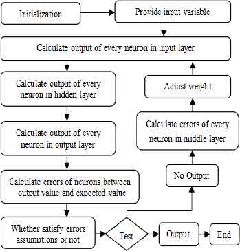
Arithmetic flow chart of BP neural network
2.2. The theory overview of Elman neural network
Elman neural network put forward by Elman, is a typical global feed forward local recurrent26. In fact, Elman neural network can be seen as a convergence network linking local memory suit and local feedback mechanism. The structure of Elman neural network includes input layer, hidden layer, connection layer and output layer. The connection layer is composed of connection units, which has a delaying effect on previous samples data. The function of connection layer mainly centers on memorability, which reflects a mixed influence coming from the previous state of hidden layer and the current input by the use of linking neurons and adjusting weight between hidden layer and connection layer.
In Fig. 3, all variables are at k time. x(k) is the output result of hidden layer, xC(k) is the output result of connection layer, W1 is weighting matrix connecting connection layer and hidden layer, W2 is weighting matrix connecting input layer and hidden layer, W3 is weighting matrix connecting hidden layer and output layer, α is automatic connection feedback factor and satisfied with the inequality 0 ≤ α < 1, y(k) is the output value of output layer. The relationship of variables can be written as expression (7), (8) and (9).
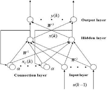
The structure of Elman Neural Network
Let eElman be an error function of Elman neural network, which is shown as expression (10).
In expression (11), (12) and (13),
Fig. 4 shows the whole running process of Elman neural network. After initializing simulation environment, the original sample data are imported into input layer. Then the calculated results gotten from input layer are loaded into hidden layer. When the output value of every neuron in hidden layer is calculated, these data can be entered output layer. The last results will be imported connection layer and enter hidden layer again together with the calculated results coming from input layer. After a series of circulation process, the errors between final values in output layer and expected values are computed. If the errors can be acceptable, the running process of Elman neural network will be terminated. In another situation, the signal weight which connects with neurons in different layers will be adjusted. Then final values in output layer will be imported input layer once more. The running process of Elman neural network will stop until the errors between final values in output layer and expected values can be acceptable.
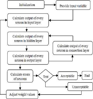
Arithmetic flow chart of Elman neural network
3. Differential analyses of neural networks based on stock price index in China
3.1. The trend of Chinese stock market based on BP neural network
As there are two stock exchanges in China: Shanghai Stock Exchange and Shenzhen Stock Exchange, the CSI 300 is a capitalization weighted stock market index showing the performance of 300 stocks traded in the Shanghai and Shenzhen Stock Exchanges. In order to study the overall trend of Chinese stock market, this paper uses the CSI 300 index as research variable from May 13th, 2010 to June 30th, 2014. The selected data are comprised of 1000 samples, which are divided into two parts: training data and testing data. Specifically, the former 800 samples are chosen as training data, and the latter 200 samples are chosen as testing data. In order to make clear the relationship between the sample value and the predicted value, let’s suppose that the input layer has four neurons, and the output layer has one neuron.
For the sake of improving the prediction performance of neural network, it is necessary to normalize all sample data by expression (17).
BP neural network having input layer, hidden layer and output layer, can fit any mapping relationship between variables. But it is difficult to determine the numbers of neurons in hidden layer, which have relation with the numbers of input suits and output suits. If the numbers of neurons in hidden layer are too few, the information acquired by neural network may be limited. If the numbers of neurons in hidden layer are high, learning process is too longer and error may be not an optimum value. Theoretically, the numbers of neurons in hidden layer can be calculated by expression (18) 27.
From expression (18), the numbers of neurons in hidden layer are Hneurons, the numbers of input variables are Nin, the numbers of output variables are Nout, is constant ranging from 1 to 10.
Considering that the numbers of neurons may have several possibilities in hidden layer, mean squared error of BP neural network is calculated in Table 1.
| Neurons | Epochs | MSE |
|---|---|---|
| 4 | 109 | 6.27e-4 |
| 5 | 35 | 6.44e-4 |
| 6 | 79 | 6.46e-4 |
| 7 | 425 | 6.04e-4 |
| 8 | 332 | 5.98e-4 |
| 9 | 1116 | 5.89e-4 |
| 10 | 961 | 5.74e-4 |
| 11 | 527 | 5.62e-4 |
| 12 | 1324 | 5.70e-4 |
Comparison results in different numbers of neurons
Some parameters of Table 1 need to be explained further. Neurons show the numbers of neurons in hidden layer. Epochs indicate the maximum training frequencies in learning process. MSE represents mean squared error. The optimal numbers of neurons in hidden layer should make MSE as smaller as possible. Finally the neurons are selected to be equal to 11.
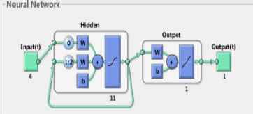
In this case, MSE is equal to 5.62e-4. The model of BP neural network established ultimately can be seen in fig. 5.

The model of BP neural network
Fig. 6 shows dynamic feature of MSE. When training process arrives at epochs 527, training result represents the best performance. Many training algorithms can be selected to train samples in BP neural network. Since the scale of sample data are basically moderate, LM algorithm having a rapid speed of convergence and a small amount of storage, is chosen in the process of training samples.
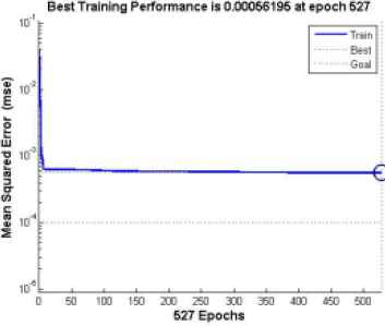
The dynamic change of MSE (BP neural network)
A better fitting effect can be seen in Fig. 7 where goodness of fit reaches 0.99471. The conclusion shows that the neural network after training has a better performance of regression.
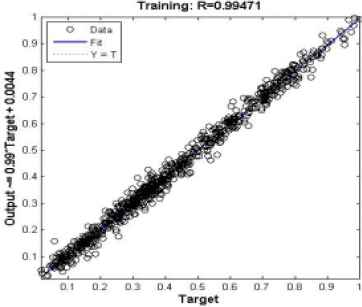
The fitting state of training data (BP neural network)
Then, training sample vectors are obtained by using the last 200 samples data. Since the relative error of training sample reflects the deviation degree between predictive value and actual value, the sign of relative error only shows the deviation direction of predictive value. The fluctuation range of relative error can be seen in Fig. 8.

The change of relative error between actual value and predictive value (BP neural network)
According to the data of Fig. 8, some features of relative error can be found when the sign of relative error is no consideration. The mean value of relative error is equal to 1.46 % and the variance of relative error is equal to 1.37%. In addition, the maximum of relative error is 5.82%.
Two curves can be seen in Fig. 9, the actual curve of original samples data and the prediction curve of BP neural network. The actual curve of original samples data is comprised of many red color plus signs, and the prediction curve is comprised of many blue dot marks. Seen from Fig. 9, two curves have a similar fluctuation tendency and a good fitting effect.
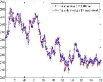
Prediction curve of BP neural network
3.2. The tendency of Chinese stock market based on Elman neural network
For the same reasons, all sample data need to be normalized in the process of applying Elman neural network. In order to compare the differences between BP neural network and Elman neural network, this paper chooses the same samples data to forecast the trend of CSI 300 index. Then, as before, let’s suppose that the input layer has four neurons, that is to say the current price is calculated by the previous prices from the first period to the fourth period. The sizes of samples data are 1000, which are divided into 800 training samples and 200 testing samples.
Due to specific characteristics of Elman neural network, hidden layer needs more neurons than those of other neural networks in solving practical problems. If the quantity of neurons in hidden layer is too small, Elman neural network will have a small chance of discovering appropriate weight. In light of that, the quantity of neurons in hidden layer is set to 11, which is also the same as BP neural network. Fig. 10 reveals network structure of Elman neural network.
The model of Elman neural network
Since the convergence speed of LM algorithm is too fast, it does not perform well in the Elman neural network. Moreover, standard gradient descent algorithm only relates to the adjustment of negative gradient direction at the current moment without involving the changes of gradient direction in the earlier period. For the sake of overcoming the disadvantages of standard gradient descent algorithm, the momentum gradient descent algorithm is selected as the learning algorithm of Elman neural network.
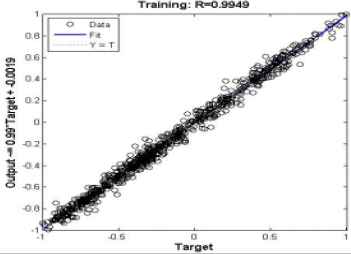
To compare differential performance of different neural networks, various parameters of Elman neural network are the same as the parameters of BP neural network. Fig. 11 shows that network training reach an expected error level at epoch 1998. The confirmation coefficient on goodness of fit calculated by training data is equal to 0.9949 in Fig. 12. As goodness of fit is high, the model after training relative accurately reflected the relationship of samples data.
The dynamic change of MSE (Elman neural network)

The fitting state of training data (Elman neural network)
In Elman neural network, training data are used for network training in the first place, and then testing data are used for network testing. In Fig. 13, the results of testing data indicate that the fitting performance of the predictive value of Elman neural network and the actual value of CSI 300 index is very significant.
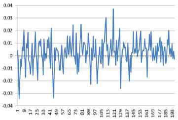
The relative error between actual value and predictive value (Elman neural network)
After training samples data, the relative error between actual value and predictive value of Elman neural network can be calculated. Fig. 13 shows the fluctuation range of relative error. This relative error is from -0.04 to 0.04.
And mean relative error is equal to 0.86% and the variance of relative error is equal to 0.51% after calculating testing samples regardless of the sign of relative error. Because mean relative error is very low, Elman neural network has an extraordinary performance in terms of analyzing CSI 300 index in Fig. 14.
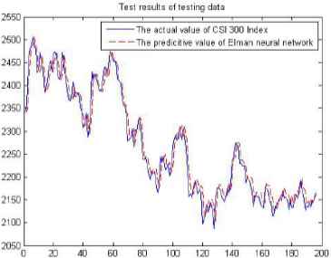
Test results of testing data
3.3. The difference between BP neural network and Elman neural network
In theory, neural network has strong non-linear mapping ability, which can simulate complex nonlinear relations between data. In order to carry out a thorough study on the difference between BP neural network and Elman neural network, CSI 300 index coming from Chinese stock market is used as the research sample. On the whole, two kinds of neural networks have the better fitting performance. But some significant differences can be easily found in the above analysis process. After differential analysis in the following aspects, analytical results can be summarized and shown in Table 2.
| Network Type | BP | Elman | |
| Epochs | 527 | 1998 | |
| MSE | 0.06% | 0.27% | |
| Confirmation Coefficient | 0.9947 | 0.9949 | |
| Relative Error | Fluctuation Range | (-0.06,0.06) | (-0.04,0.04) |
| Mean | 1.46 % | 0.86% | |
| Var | 1.37 % | 0.51% | |
The performance difference between neural networks
Firstly, the variation curve of MSE is different between BP neural network and Elman neural network. Network training satisfies error requirement after 527 epochs in BP neural network, and the training error is equal to 0.06%. But the speed of convergence of network training is slower in Elman neural network. After 1998 epochs, the goal of network training is achieved and the training error is equal to 0.27%. Although the training error in Elman neural network is larger than that in BP neural network, both are smaller in general and less than 0.01. This suggests that the effect of network training is extremely good by using training data, no matter BP neural network or Elman neural network.
Secondly, two kinds of neural networks have similarly higher confirmation coefficient of training samples. Confirmation coefficient that measures the correlation between variables in regression model, reflects the degree of sample regression line simulating sample data. A higher confirmation coefficient indicates that sample regression line has a better fitting effect on sample data. That confirmation coefficient of training samples is equal to 0.9947 in BP neural network manifests the trained neural network model having a strong ability in simulating sample data. Meanwhile, the simulation result of sample data reaches a similar conclusion in Elman neural network, where the calculated confirmation coefficient is equal to 0.9949. No matter what type of neural networks, the confirmation coefficient of training samples has obviously statistical significance. And the confirmation coefficient in BP neural network equals approximately to that in Elman neural network. Thus such a conclusion can be drawn that both BP neural network and Elman neural network have a great ability of fitting training samples.
Thirdly, the noticeable differences between neural networks appear in testing results of training data. These differences mainly focus on statistical characteristics of relative error between actual value and predictive value. The relative error between actual value and predictive value in BP neural network has a wider range from -0.06 to 0.06 comparing with the fluctuation range of relative error from -0.04 to 0.04 in Elman neural network. Moreover, testing results of training data in BP neural network has the higher mean relative error and the variance of relative error. These differences can be seen in Table 2 where Elman neural network has the significantly lower mean and variance of relative error. Therefore, Elman neural network has better performance in terms of data fitting between actual value and predictive value.
4. Conclusions
In stock market, many factors may affect fluctuation of stock price. Since stocks are issued by stock companies, the prices of stocks are influenced by the corporate operational performance at first. As a general rule, the better operational performance can make stock price rise, and the worse operational performance can make stock price drop. Moreover, other factors outside the corporate also affect stock price, such as political environment, interest rate change and economic cycle. It is clear that each stock is influenced by many factors, so the research on all stocks in trading market becomes more complicated. As stock market can only be seen as a complicated nonlinearity system, traditional prediction method is difficult to reveal the inherent rules of price fluctuation.
This paper adopts different kinds of neural network to analyze the difference of simulation results in terms of forecasting stock price trend. In the same simulation environment, BP neural network and Elman neural network are used for comparing prediction performance based on Chinese stock market. As BP neural network belongs to feedforward neural network, the output value of network is only influenced by the current input value and weight matrix. The disadvantage of BP neural network is that the former output value has no effect on the current output value in the analysis of sample data. But in stock market, the trend of current data may be influenced by the previous data over and over again. Hence feedback neural network, which imports the former output value together with the current input samples into network model, can effectively overcome the disadvantage of feedforward neural network. In the aspect of forecasting time series trend, Elman neural network as a kind of feedback neural network has obvious advantage of fitting sample data comparing with BP neural network in theory. In fact, when CSI 300 index is used to analyze performance difference between neural networks, the same conclusion can be arrived by simulation models. The data in Chinese stock market again suggests that the prediction performance of Elman neural network is significantly better than that of BP neural network.
BP neural network model and Elman neural network model can be regards as numerical neural networks in this paper, which directly show dynamic characteristics of CSI 300 index in numerical form. But, trained neural networks coming from BP neural network and Elman neural network unavoidably also have “Black Boxes” structural features. For analyzers, it is difficult to understand the trained neural networks. So, symbolic knowledge extraction from trained neural networks is generally used for solving “Black Boxes” problems appearing in neural networks28. Through structural analysis method and performance analysis method, symbolic knowledge can be extracted from trained neural networks29. The main idea of the first method is that rule extraction is regarded as a searching process. In this searching process, the structures of trained neural networks will be mapped into the correspondent rules. Another method sees neural network as an entirety, without thinking about the structures of trained neural networks in the process of rules extraction. Therefore, in the future research, we will consider the possibility to use symbolic neural network models for representing as symbolic rules relationship between investors and price fluctuations in Chinese stock market.
Acknowledgements
Thanks to the reviewers for their useful comments, and National Natural Science Foundation of China (No. 71371051), the Fundamental Research Funds for the Central Universities and the Jiangsu Innovation Program Foundation for Graduate Education (No. KYZZ_0081).
References
Cite this article
TY  - JOUR
AU  - Binghui Wu
AU  - Tingting Duan
PY  - 2017
DA  - 2017/01/01
TI  - A Performance Comparison of Neural Networks in Forecasting Stock Price Trend
JO  - International Journal of Computational Intelligence Systems
SP  - 336
EP  - 346
VL  - 10
IS  - 1
SN  - 1875-6883
UR  - https://doi.org/10.2991/ijcis.2017.10.1.23
DO  - 10.2991/ijcis.2017.10.1.23
ID  - Wu2017
ER  -