
A decision tree based approach with sampling techniques to predict the survival status of poly-trauma patients
- DOI
- 10.2991/ijcis.2017.10.1.30How to use a DOI?
- Keywords
- Trauma patients; Survival prediction; Decision trees; Imbalanced classification problems; Sampling Techniques
- Abstract
Survival prediction of poly-trauma patients measure the quality of emergency services by comparing their predictions with the real outcomes. The aim of this paper is to tackle this problem applying C4.5 since it achieves accurate results and it provides interpretable models. Furthermore, we use sampling techniques because, among the 378 patients treated at the Hospital of Navarre, the number of survivals excels that of deaths. Logistic regressions are used in the comparison, since they are an standard in this domain.
- Copyright
- © 2017, the Authors. Published by Atlantis Press.
- Open Access
- This is an open access article under the CC BY-NC license (http://creativecommons.org/licences/by-nc/4.0/).
1. Introduction
Poly-trauma patients are those who suffer from several injuries, which have been produced by energy exchanges 1, for instance, car crashes or falls. Survival prediction of these patients is a good indicator of the quality of an emergency system, since a number of saved patients greater than the number of patients expected to survive is an indicator of a high quality emergency service. A good emergency system is aimed at both saving as many patients’ lives as possible and trying to treat them in such a way that after their recovery they will have the best possible health condition. Moreover, the latter fact leads to a reduction of the expenses derived from the subsequent treatments given to the patients that survive to their damages.
Hence, in order to asses the quality of an emergency service, it is interesting to develop a model for predicting the survival of patients arriving at the emergency services. This model can be subsequently used to objectively compare the scores obtained by different emergency systems when using it. To do so, doctors usually apply techniques that translate the severity of the injuries into a number, which represents the probability of patients to survive to their injuries. Therefore, these techniques can be seen as classification systems 2 because their outcomes have two different values, namely, survive and die. Nowadays, the usage of intelligent systems has become a widely used solution to tackle classification problems 3,4,5. Specifically, the standard intelligent system used by doctors to deal with the survival prediction problem is the logistic regression 8,9, which obtains accurate results but it does not provide an explanation of its predictions.
Fortunately, the number of poly-trauma patients who survive exceeds the number of those who die. In data mining, this fact is know as the imbalanced problem 10, since there are more examples (patients) belonging to one class, which is known as majority class (survive in our case), than to the remaining one, which is known as minority class (die in our problem). Tackling imbalanced problems using intelligent systems is one of the current challenges in the topic 11, since classifiers tend to predict the majority class for most of the examples and consequently, they fail most of the examples belonging to the minority class. In order to improve the obtained accuracy in both classes, sampling techniques 12 are usually applied before learning the classifiers.
The goal of this work is to deal with this problem applying intelligent systems capable of providing an interpretable model for predicting the survival status (survive or die) of poly-trauma patients. In this manner, the system will make predictions and it also will help to understand them as well as enabling doctors to analyse which are the key variables involved in this type of problems. Using this knowledge, health managers could try to adapt the trauma care units and/or the service protocol to improve the quality of the treatments for the sake of increasing the survival rate of their patients. Additionally, sampling techniques will be applied to try to improve the performance of the classifiers by balancing the number of patients of both classes for the learning process.
Taking into account the previous considerations, we propose the usage of the C4.5 decision tree 13 because it obtains accurate results and it creates an interpretable model. Specifically, the generated model is represented by a tree, which is suitable for this application since doctors frequently use protocols written in tree form. Consequently, the knowledge can be easily interpreted by the medical staff. Furthermore, we apply sampling techniques including several under-sampling methods 14,15,16,17, SMOTE 18 as representative of over-sampling techniques and two hybrid approaches that combine the two previous options. Additionally, we also study the effect of two recent splitting methods 19,20 used to conform the different folds used in the evaluation process.
The experimental study is conducted using the patients stored in the Major Trauma Registry of Navarre (MTRN) 21. Specifically, the MTRN is composed of 378 patients treated at the emergency services of the Hospital of Navarre during 2011 and 2012. The quality of the classifiers is measured using three well-known performance metrics: the accuracy rate, the Area Under the ROC Courve (AUC) 22 and the geometric mean 23, which quantifies the trade-off between the sensitivity and specificity rates. The obtained results show that the C4.5 decision tree provides a competitive performance when it is compared with the logistic regression approaches 8,9, whereas it also allows doctors to study the main variables affecting the survival or death of poly-trauma patients. Furthermore, it is also observed that the usage of sampling techniques allows the performance of the system to be notably improved.
The remainder of the paper is organized as follows: in Section 2 the features of the dataset and the collection of data are explained as well as a description of the standard methods used to tackle the current problem. Sections 3 and 4 introduce the proper background about imbalanced datasets including the sampling techniques and the C4.5 decision tree algorithm, respectively. Our proposed methodology to tackle the survival prediction problem is described in detail in Section 5. The obtained results and the corresponding analysis is presented in Section 6. Finally, in Section 7 we draw the main conclusions of the paper.
2. Framework of the poly-trauma patients survival prediction problem
Poly-trauma patients are persons who have several injuries, which imply a risk of death. It is one of the most common causes of death among people under forty and it also implies high economic costs for health care centres 24,25,26. The survival rate of these patients is a good indicator of the quality of the emergency system of a health center. Specifically, there exists an approved medical treatment for such patients and there is a relationship between therapeutic measures and the outcome, which can only take two values: survive or die.
The aim of any quality control system of trauma care centres is to perform a continuous and measurable improvement of the treatments used to treat traumatized patients. To this aim, the information obtained from all the poly-trauma patients that were taken care of is stored in a Major Trauma Registry (MTR) 21. A MTR is a source of a opportune, accurate and complete information that allows one to continuously monitor the assistance’s process in trauma care units. A well-designed MTR helps health managers to analyse the information to try to discover aspects that can be improved with the aim of both enhancing the quality of life of poly-trauma patients and coordinating the different services involved in the care centres. Such monitoring and quality control has allowed the reduction of both the mortality and the disability rates of these patients in developed countries in recent years 27.
The Emergency Department of the Hospital of Navarre made a study between 2001 and 2003 that allowed to develop and validate the MTR of Navarre * (MTRN). This registry is based on the Utstein template 28, which establishes the variables to be collected. Some of them are easily obtained like the age or the gender of patients whereas other ones are based on the severity of the injuries like the Injury Severity Score (ISS) 29, the New Injury Severity Score (NISS) 30, the Revised Trauma Score (RTS) 31 or the Triage Revised Trauma Score 31. The most relevant variables (among the ones determined by the Utstein template) from a clinical perspective are introduced in Table 1.
| Survival | Age | Gender |
| Cardiac arrest | Pre-hospital care | Pre-hospital intubation |
| Type of intubation | Pre-hospital inmovilization | Pre-hospital and hospital RTS |
| Pre-hospital and hospital TRTS | ISS | NISS |
| Glasgow | Respiratory rate | Arterial pressure |
| Time until first CAT scan | Time until first key surgical intervention | Type of first key surgical intervention |
Most relevant variable stored in the MTRN.
We have to point out that not all the poly-trauma patients are stored in the MTRN. The excluding criteria are the following ones:
- 1)
The NISS value is less than 15.
- 2)
The period of time between the injury and the admission to the hospital is greater than 24 hours.
- 3)
The patient has been drowned.
- 4)
The patient has been hanged.
- 5)
The patient has been burnt.
2.1. Standard solutions based on intelligent systems
One of the main aims of a MTR, so that both patient survival and data collection can be improved, is to compare the results obtained in different institutions at any level (regional, national or international) 32,33.
For this aim, intelligent systems are usually applied. In fact, the standard method in this domain is the Trauma and Injury Severity Score (TRISS) 8. This system is based on a logistic regression, which is applied to estimate survival probabilities of patients. Specifically, the input features considered by this model are the ISS 29, the RTS 31 and the categorized data of age.
Furthermore, the medical staff of the Hospital of Navarre developed their own model that was also based on a logistic regression. Doctors determined the input features to be used and presented several models in 9. The most accurate one considered as input variables the age, the Revised Trauma Score (RTS) and the New Injury Severity Score (NISS) and the morbidity, which was binarized.
Finally, another important method used in this field is the Revised Injury Severity Classification (RISC)34. This model considers laboratory values like base deficit, haemoglobin concentration and thromboplastin time for the first time, as well as medical interventions such as cardiopulmonary resuscitation (CPR) 35. This allows for a more precise description of the prognosis of trauma patients. However, several limitations of the RISC model have been identified, which have led the authors to develop a new updated version of the model known as RISC II 36. However, doctors of the Hospital of Navarre conducted an study where they proved that the prediction capability of RISC II is less than their own method (introduced in the previous paragraph).
3. Imbalanced datasets problem
An imbalanced dataset classification problem 10 occurs when the number of examples belonging to the different classes is notably different. Focusing on classification problems composed of only two classes, the class having the largest number of examples is known as the majority class (it is also named negative class) whereas the remainder one is called minority class (or positive class). A wide number of real-world classification problems present the imbalanced issue 3,37,38,39.
This problem is currently a challenge in classification 11 because it has several features implying extra difficulties to learn suitable classifiers. Among them, two well-known problems are the overlapping between the examples of the different classes and the small disjuncts 40, which are depicted in Figure 1.
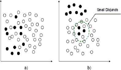
Two problems in imbalanced datasets: a) overlapping between classes; b) small disjuncts.
In addition to the previous problems, standard classifiers using the accuracy rate (number of correctly classified examples divided by the total number of examples) in their learning process usually have a bias in favour to the majority class. This is due to the fact that the larger the imbalance ratio the better will be to classify correctly the examples of the majority class in order to obtain a good accuracy rate. Consequently, the relevance of a right classification of the examples belonging to the minority class will decrease. This is a huge problem when the class of interest is the one with the less number of examples like, for instance, when tackling a problem in which patients have to be diagnosed to know whether they suffer from cancer or not. Fortunately, the number of patients who do not have cancer is several times greater than the one of those who have it. In this situation there would be a trend to predict that the patients do not have cancer but this fact would imply misclassifying many patients who really suffer from it. Therefore, the accuracy rate would be high although the classifier is not working properly.
In the remainder of this section we firstly introduce the performance metrics used in this type of classification problems to avoid the aforementioned problem of the accuracy rate. Then, we describe several sampling methods used to balance the number of examples of the different classes before generating the classifier, which imply that both classes will be equally important in the learning process.
3.1. Metrics for imbalanced problems
We have already mentioned that the standard accuracy rate is not a suitable performance metric for this type of classification problems. Its usage could provoke a bad analysis of the quality of the classifier as illustrated in the following example. Let imagine we have to tackle a two-class problem in which one of the classes has 975 examples and the remainder one has only 25. If the classifier assigned all the examples in the majority class it would obtain a 97.5% accuracy rate, which is a good performance. However, this classifier has miss-classified all the examples of the minority class and therefore, it is not solving properly the problem.
To cope with this problem, we recall two well-known metrics that are built from a confusion matrix (see Table 2), which stores the number of correctly and incorrectly classified examples for each class.
| Positive class prediction | Negative class negative | |
| Positive real class | True Positive (TP) | False Negative (FN) |
| Negative real class | False Positive (FP) | True Negative (TN) |
Confusion matrix for a two-class problem.
The first appropriate metric for imbalanced classification is the Geometric Mean (GM) 23, which takes into account the accuracy obtained for each class of the problem (see Eq. 1).
The second widely used metric for this type of problems is the Area Under the Receiver Operating Characteristic (ROC) curve (AUC) 22. This curve is constructed computing one ore more (TPrate,FPrate) pairs, where
- •
All the examples are classified and their probabilities, provided by the classifier, of belonging to the positive class are taken.
- •
The previously obtained probabilities are sorted in ascending order.
- •
For each probability value, pi
- •
All the examples having a probability less than pi are predicted as negative.
- •
The examples whose probabilities are greater or equal than pi are predicted as positive.
- •
- •
The confusion matrix for each probability value, pi, is obtained.
- •
Finally, the pair of values (TPrate,FPrate) is computed form the confusion matrix.
Once the ROC curve is generated its area is computed and it is used as the performance of the classifier. Therefore, this measure depends on the variety and quality of the probabilities returned by the classifier.
3.2. Sampling methods to pre-process imbalanced datasets
We have already mentioned that sampling techniques 12 are widely used to deal with imbalanced datasets. The aim of this techniques is to balance the number of examples belonging to the different classes. In this manner, when learning the classifier all the classes have the same importance and the bias in favour to the majority class is avoided. All the sampling methods fall into one of the following three groups.
- 1.
Under-sampling methods: This methodology pre-processes the data by removing examples belonging to the majority class. Among the techniques belonging to this methodology we can stress the following ones:
- •
Tomek links 14: Let Ei and Ej be two examples belonging to different classes and let d(Ei,Ej) be the distance between them. A pair (Ei,Ej) is called a Tomek link if there is not an example El, such that d(Ei,El) < d(Ei,Ej) or d(Ej,El) < d(Ei,Ej). This method can be used as an under-sampling method (it only removes the example of the Tomek link belonging to the majority class) or as a cleaning method (both examples are removed).
- •
Condensed Nearest Neighbour rule (CNN) 15: Let E be the set of all the examples and let Ê be a subset composed of all the examples of the minority class and one of the majority class, which is randomly selected. Then, the 1NN algorithm † is used to classify all the examples in E using Ê as training set. Next, the misclassified examples are moved to the subset Ê. This process is repeated until all the examples E are correctly classified. When the process is finished, Ê is a consistent subset and it is appropriate to start learning from it because it contains both the examples of the minority class and the most difficult ones (close to the boundaries) from the majority class.
- •
One-Sided Selection (OSS) 16: This method combines the two previously described approaches, that is, it firstly applies the Tomek links method (as under-sampling) and then, it executes CNN to remove majority class examples that are far away from the decision border.
- •
CNN + Tomek links: The same schema of the OSS method is followed but it changes the order in which both methods are applied.
- •
Neighbourhood CLeaning rule (NCL) 17: This method is based on Edited Nearest Neighbor (ENN) 43. For each example Ei, its three nearest neighbours are obtained. In case the three nearest neighbours contradicts the class of Ei, the examples belonging to the majority class are removed, that is, it can be deleted either the example Ei or the three nearest neighbours.
- •
- 2.
Over-sampling methods: This methodology pre-processes the data by generating new examples belonging to the minority class. The most used technique in this group is the Synthetic Minority Over-sampling Technique (SMOTE) 18. The created examples are the result of interpolating the values of several minority class examples that are close to each other. The detailed procedure is the following: let xi be an example of the minority class and n1,…,n4 be its four nearest neighbours. To generate a new example, one of the four neighbours is randomly selected. Then, for each attribute, the difference between the values of xi and the selected neighbour multiplied by a random number (in [0,1]) is added to the value of xi. Consequently, the new example will be located between the two values that have engendered it.
- 3.
Hybrid methods: The techniques belonging to this group combine under-sampling and over-sampling methods. Among them we can stress the two following ones:
- •
SMOTE + Tomek Links: this method generates minority class examples using SMOTE and then, in order to create better-defined class clusters, Tomek links is applied as cleaning method.
- •
SMOTE + ENN: this method follows the same process than the previous one but, in this case, ENN is used to remove examples belonging only to the majority class. ENN applies the same process than NCL but it removes the majority class examples when the class of the analysed example differs from that of at least two of its three nearest neighbours.
- •
4. C4.5 decision tree
In this section we describe in detail the C4.5 decision tree 13, which is an intuitive and interpretable tool to classify the patients. The relevance of this classifier is shown through the wide range of real-world applications in which it has been used 44,45 as well as the fact that it is considered as one of the top ten techniques in data mining 46.
A decision tree is an interpretable classifier composed of nodes connected by branches as depicted in Figure 2. There are three different types of nodes:
- 1)
Root node: It is the beginning of the decision tree (top of the decision tree) because it has not input branches. That is, all the examples (patients) arrive to this node, since no splitting criteria is applied yet.
- 2)
Internal nodes: This type of node has both input and output branches. For this reason, they are decision nodes because they specify an attribute to be tested and according to the value of the example the proper output branch is followed.
- 3)
Leaf nodes: They are the last nodes of the decision tree and they do not have output branches. They assign the example the most probable class of the leaf, which is determined in the learning process. In Figure 2, the leaves are the dotted and bold stressed nodes. Dotted nodes predicts the Die class (label D) whereas bold-faced nodes assigns Survive class (label S). In both cases it is also shown the probability (depicted in terms of percentage) of the class in the leaf. This probability is computed using the Laplace correction 47, which is obtained computing
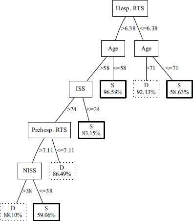
An example of a decision tree generated by the C4.5 approach to tackle our problem.
The generic learning process of the C4.5 decision tree is shown in Algorithm 1. The key points of this algorithm are explained below (see 13 for details).
- •
Attribute selection for each node: the best attribute is the one maximizing the gain ratio, which computes the reduction in entropy if we used it to ramify the tree. This heuristic criteria corrects the tendency in favour of the attributes having a larger number of possible values to branch on, which is the problem derived from the usage of the information gain in the ID3 decision tree 48. When the best attribute is determined, the node is ramified using as many branches as values the attribute has.
- •
Management of numerical attributes: C4.5 provides a method to determine the best threshold for the numerical attributes in each node. To do so, the possible numerical values are sorted and the value that maximizes the information gain is selected as the threshold.
- •
Treatment of missing values: this method allows one to handle attributes having missing values. This feature is crucial in our problem, since some fields, like the information related to dates (arrival at the hospital, surgery, etc..), is usually unknown. C4.5 instead of ignoring those examples having missing values assigns them to each branch of the node with a weight, which is the percentage of the examples (used to learn the tree) that followed each branch.
- •
Stopping conditions: The recursive learning is made until one of the following conditions is fulfilled:
- •
The node is pure, that is, all the examples arriving it belong to the same class.
- •
The attributes that can be used to split the tree provide zero information gain.
- •
All the attributes have been already used.
- •
There are no examples arriving at the node.
- •
Some branch does not have enough examples (minimum number of examples per branch condition).
- •

C4.5 algorithm
Once the C4.5 learning process is finished, C4.5 applies a pruning method to improve the generalization ability of the created model. The process is called pessimistic pruning and it uses the training examples to evaluate for every non leaf sub-tree whether it is beneficial to prune it by the best possible leaf or not. That is, if the estimated error achieved when replacing the sub-tree by a leaf was equal or smaller than the original tree, the leaf would replace the sub-tree (the original tree is therefore pruned).
Finally, the process to classify new unseen examples using the generated decision tree is straightforward. Starting from the root node, the attributes of the reached nodes are evaluated and the example is driven by the branches matching its values. The process is finished when a leaf node is reached, which contains the class assigned as the prediction for this example and the probability. The process is slightly different when the example has missing values for any of the arrived nodes. In this situation, the example is driven for all the branches in proportion to the percentage of the training examples which followed this branch. As a consequence, the example reaches several leaves implying that the final prediction is made based on the weighted sum of the leaves’ probabilities.
5. Tackling the survival prediction problem using the C4.5 decision tree and sampling methods
In this paper, we apply the Knowledge Discovery process (KDD) (see Figure 3) in order to deal with the prediction of survival prediction problem. As can be observed, the 3 first steps of the KDD process consist in preprocessing the data to improve it so as the applied data mining technique is able to obtain the best possible knowledge.

KDD process.
We must recall that the aim of the paper is to be able to solve the problem using an interpretable classifier, which will enable doctors to study the learnt model for the sake of trying to discover factors that allow them to improve the measures to be applied for these patients. In this paper, we have used the following techniques:
- 1.
Data cleaning: we firstly delete incoherent values of the examples.
- 2.
Outlier detection: a value that is very different from the remainder ones is considered to be an outlier. These values can be generated by some kind of error and hence, they must be removed since they can negatively affect the final results. In order to detect outliers, we apply the Grubbs two-sided test 49 setting the level of confidence to α = 0.05.
- 3.
Variable selection: The need of this process arises from the fact that it is possible to have highly correlated attributes or attributes without importance to make decisions. Therefore, we carry out a correlation study to select those input variables which are correlated with the output of the problem, since they will be the most suitable variables for the prediction. Specifically, we use non-parametric correlation since our variables are not normally distributed and therefore, linear correlation does not fit them. We have selected the Spearman correlation, which measures the relationship between two continuous variables. Those variables having a p-value under 0.05 are selected as relevant for our problem.
- 4.
Sampling techniques: in case the classification problem suffers form an imbalance problem, as described in Section 3, it may be necessary to apply techniques to balance the data so that the learning process of the intelligent system does not favour to the majority class. In this manner, the created model could enhance the classification performance.
- 5.
Intelligent system generation: we have selected the C4.5 decision tree 13 because, as described in the previous section, since it fulfils all the requirements demanded by doctors, namely, it provides an accurate and interpretable model and it allows one to handle missing values. The returned value is the probability of the patient to belong to the class of the reached leaf, that is, to survive or die.
We have made a modification on the Laplace correction used by C4.5 to compute the probabilities of the leaves. The reason is that this correction assumes that the class distribution is balanced, that is, each class has the same number of examples. This is not our case since, as we have pointed out, there are more patients who have survived than those who have died. In order to take into account it, we propose to compute the probabilities of the leaves in a different way depending on their classes. For those leaves labelled in the majority class we apply
- 6.
Visualization: to graphically show the generated decision trees we have used the dot graph oriented language. Specifically, we have added a function in our code to translate the decision tree in the dot code and finally, we have used the graphviz‡program to compile and show them. An example of the decision trees visualized with this tool is depicted in Figure 2.
6. Results
In this section we show the results achieved by the proposed methodology to deal with the survival prediction of poly-traumatized patients.
In first place we show the differences achieved by the C4.5 decision tree with and without the Laplace correction besides our proposed modification to take into account the class distribution (Section 6.2).
Then, we compare the results provided by our proposal versus the ones obtained when applying the linear regression defined by the medical staff of the hospital of Navarre 9 as well as the standard TRISS 8. In this scenario we carry out the experiments using all the pre-processing methods to deal with the imbalanced datasets problem described in Section 3 (Section 6.3).
Finally, we show the impact of the splitting method used to perform the cross validation scheme selected to measure the performance of the approaches (Section 6.4).
The experimental framework used to conduct all the experiments is presented in Section 6.1.
6.1. Experimental framework
The dataset contains information of 378 patients who have been treated at the Hospital of Navarre between 1 January, 2011 and 31 December, 2012. Those patients were stored in the MTRN as explained in Section 2. The collected variables are those defined by the Utstein model 28. Among the 378 patients, 308 survived to their injuries, which is the 81.48% of the patients, whereas the remainder 70 ones died, which is the 18.52% of the patients.
In order to evaluate the performance of the classifiers, one of the most used methods is the k-fold Stratified Cross-Validation model (k-SCV). In our case, we have applied the 10-SCV. That is, the dataset is split in ten folds that have the same number of patients among them and they maintain the percentage of patients of each class of the whole dataset. Then, the combination of nine of them is used to learn the classifier and the remainder one is used to test it, that is, to simulate unseen patients. This process is repeated ten times by using a different fold for testing in each run. Therefore, after all the repetitions all the patients will be considered as unseen cases implying a good indicator of the quality of the classifier to tackle the problem. As final result we compute the average performance over the ten testing folders.
In each fold we have considered three common metrics in classification, the accuracy rate, the geometric mean (GM) and the Area Under the ROC Curve (AUC). The former is standard in classification problems whereas the two remainder ones are more appropriate for imbalanced datasets as it is our case. Furthermore, we also compute for each fold the number of leaves of the generated decision tree so as to measure information related to the interpretability of the generated model.
The parameters used in C4.5 have been the default ones. We have applied the pruning process using 0.25 as confidence level whereas the minimum number of examples per leaf is 2.
Regarding the two logistic regression methods used in the comparative study we use the standard configuration of TRISS and for the logistic regression defined by the medical staff of the Hospital of Navarre, they suggested us to binarize the values of the numerical variables in order to ease the interpretation of the results from a clinical point of view 9. Both the variables used for the logistic regression and the binary values assigned after the binarization process are shown in Table 3. The interpretation of the binary values is that a value of 1 means that the condition implying this value is a protector factor since the survival class is encoded with the value 1.
| Variable | Original Value | Value assigned |
|---|---|---|
| Age | < 60 | 1 |
| ⩾ 60 | 0 | |
| RTS | < 7 | 0 |
| ⩾ 7 | 1 | |
| NISS | < 20 | 1 |
| ⩾20 | 0 | |
| Previous comorbidity | Healthy | 1 |
| Moderate systemic disease or severe systemic disease with constant treatment | 0 |
Values assigned for the logistic regression develop by the Hospital of Navarre.
6.2. Analysing the behaviour of the different versions of the C4.5 decision tree
In this section we want to study whether our proposed method to compute the probabilities of the leaves taking into account the Class Distribution (C4.5 CD) is able to improve the result obtained with the classical C4.5 decision tree with (C4.5 Laplace) and without (C4.5) the Laplace correction. The results obtained by the three versions of the C4.5 algorithm are introduced in Table 4, where in each row we show each method and the results obtained with the different performance measures are introduced by columns, namely, AUC, accuracy, the accuracy in each class and the GM. In the last column we also show the number of leaves that compose the generated decision tree (#leaves), which is used to report the interpretability of the tree.
| Method | AUC | Accuracy | AccMaj | AccMin | GM | #Leaves |
|---|---|---|---|---|---|---|
| C4.5 | 0.75 | |||||
| C4.5 Laplace | 0.77 | 0.84 | 0.94 | 0.43 | 0.61 | 27.4 |
| C4.5 CD | 0.80 |
Results in testing obtained with C4.5, C4.5 Laplace and C4.5 CD.
From the results shown in Table 4 we first have to point out that they are the same in three metrics, namely, accuracy, accuracy in each class and geometric mean. This is logical since the equation used to obtain the probabilities of the leaves does not affect to the final decision but to the confidence given for that prediction. Consequently, the unique measure that changes for these three techniques is the AUC. If we look at these results, we can see that both approaches to correct the probabilities excels the results of the original equation and among these two, our proposal obtains better results than that of the original Laplace correction. This is due to the fact that as we get smoother probabilities the effect to the impact of the miss-classifications becomes less detrimental in terms of AUC.
6.3. Comparing C4.5 and classical prediction survival models
This section has two aims:
- •
- •
To analyse the impact of the sampling methods described in Section 3.2 on the results provided by C4.5 as well as the logistic regression.
We must point out that the results achieved by the TRISS method are the same ones regardless of the sampling method used. This is due to the fact that TRISS does not have a learning stage, since the standard values of its parameters are derived from multiple regression analysis of the Major Trauma Outcome Study database. Consequently, it does not matter the processing made to the training set. The results obtained by TRISS are:
- •
AUC: 0.89.
- •
Accuracy: 0.86.
- •
Accuracy in the majority class: 0.94.
- •
Accuracy in the minority class: 0.47.
- •
GM: 0.66.
In Table 5 are shown the results obtained by both our proposed methodology as well as the logistic regression defined in 9. This table is composed of 9 rows and 11 columns: in each row we introduce each sampling method whereas in columns are shown in groups of two (according to the performance measure) to introduce the results of these two classifiers. The last column is again used to report the number of leaves of the created decision trees (#leaves).
| Balancing Method | AUC |
Accuracy |
AccMaj |
AccMin |
GM |
#leaves | |||||
|---|---|---|---|---|---|---|---|---|---|---|---|
| C4.5 CD | Reg | C4.5 CD | Reg | C4.5 CD | Reg | C4.5 CD | Reg | C4.5 CD | Reg | C4.5 CD | |
| None | 0.80 | 0.86 | 0.84 | 0.86 | 0.94 | 0.96 | 0.43 | 0.40 | 0.61 | 0.55 | 27.4 |
| Tomek | 0.74 | 0.87 | 0.86 | 0.86 | 0.95 | 0.97 | 0.44 | 0.37 | 0.63 | 0.53 | 11.2 |
| CNN | 0.76 | 0.88 | 0.75 | 0.74 | 0.78 | 0.72 | 0.63 | 0.81 | 0.69 | 0.76 | 20.6 |
| OSS | 0.74 | 0.85 | 0.75 | 0.77 | 0.78 | 0.78 | 0.61 | 0.71 | 0.67 | 0.74 | 7.6 |
| CNN+Tomek | 0.77 | 0.85 | 0.73 | 0.70 | 0.72 | 0.65 | 0.77 | 0.90 | 0.73 | 0.76 | 9.1 |
| NCL | 0.81 | 0.86 | 0.83 | 0.86 | 0.91 | 0.96 | 0.47 | 0.40 | 0.64 | 0.55 | 25.5 |
| SMOTE | 0.84 | 0.85 | 0.84 | 0.72 | 0.89 | 0.68 | 0.61 | 0.91 | 0.73 | 0.78 | 55 |
| SMOTE+Tomek | 0.83 | 0.86 | 0.78 | 0.72 | 0.78 | 0.67 | 0.80 | 0.93 | 0.78 | 0.79 | 31.6 |
| SMOTE+ENN | 0.85 | 0.85 | 0.78 | 0.72 | 0.80 | 0.68 | 0.71 | 0.91 | 0.75 | 0.78 | 31.3 |
Results in testing for both C4.5 and logistic regression using different sampling techniques.
To analyse the obtained results, we first study them using the performance metrics based directly on the confusion matrix (accuracy, accuracy in each class and GM) and next, in terms of AUC. To start with, from results in Table 5, it can be observed that C4.5 obtains better results than the logistic regression for 5 out of the 9 sampling techniques (and 1 tie) in terms of accuracy. In most of the cases this enhancement is based on the obtaining of a better classification for those patients who survived whereas the logistic regression provides more accurate results for patients who die. Looking at the results using the GM, we can stress that the method obtaining the best performance for patients belonging to the class die is the one obtaining a best result. Therefore, the logistic regression usually provides better results using this metric.
On the other hand, looking at the performance of both techniques using AUC, we can observe that the logistic regression always provides the best result (except with SMOTE+ENN where they tie). This result seems contradictory with the one of the accuracy rate. However, the reason behind this behaviour are the probabilities returned by the classifiers when they fail their predictions, which are used to compute the AUC. Specifically, the larger the returned probability the greater the impact on the reduction of the AUC.
This fact is observed in Figures 4 and 5, where in Figure 4 are depicted the ROC curves obtained for both techniques and in Figure 5 are depicted (increasingly sorted) the probabilities returned for the misclassified patients by them, which are 60 and 53 in case of C4.5 and the logistic regression, respectively. We have to recall that when the probability is larger than 0.5 the patients is classified as survive and otherwise as die. Consequently, from Figure 5 we can observe that most of the misclassified patients belong to the class die because the classifiers are predicting the class survive. Moreover, we can also see that C4.5 classifies, with a confidence larger than 0.8, more than 20 patients whereas the logistic regression only classifies 5 with such a large probability. This fact implies a large AUC difference in favour to the logistic regression (see Figure 4) despite it only correctly classifies 7 patients more than C4.5.

ROC curves for C4.5 CD and logistic regression.

Survival probability for misclassified examples.
Regarding the usefulness of sampling techniques we can observe the following situations:
- •
The usage of sampling techniques generally implies an increase on the accuracy of the minority class and a decrease on the one of the majority class. This fact implies a reduction in the accuracy rate and a enhancement on the GM.
- •
Under-sampling methods: CNN, OSS and CNN+Tomek do not work properly since they cause a reduction in the performance for all the measures except for GM. Tomek and NCL allows these two classifiers to improve or not notably decrease their results.
- •
SMOTE: this over-sampling technique allows these classifiers to notably raise their results in terms of AUC (logistic regression slightly worsen its results without sampling) and specially with GM.
- •
Hybrid methods: They present a similar effect than that of SMOTE. Therefore, they also enables them to obtain a large enhancement of their results using AUC and GM but they cause a notable decrease using the accuracy rate.
- •
Under sampling techniques, as expected, allows the generated decision trees to become simpler whereas a slightly increase on the trees’ sizes is implied by hybrid techniques and huge decision trees are learned when using SMOTE.
To sum up, we must stress the good synergy obtained by both classifiers with NCL, SMOTE and the hybrid techniques. With these four combinations, the obtained results are competitive with those provided by the standard TRISS approach (especially in terms of GM). Consequently, we can also observe that the combination of C4.5 with sampling techniques is able to be competitive in terms of GM with respect to the logistic regressions while it provides an interpretable model that can be easily interpreted by doctors at the hospital. Specifically, we can conclude that for C4.5 the most appropriate sampling method is SMOTE+ENN, since it allows its results to be clearly enhanced whereas it implies to maintain the number of leaves of the generated tree without using sampling methods and consequently, to maintain its interpretability.
6.4. Analyzing the impact of the splitting process in the k-fold cross validation model
In this section we want to analyse the effect on the results derived from the method applied to perform the k-fold cross validation method. This process is key since it determines the examples that are assigned to each one of the k folds. Recently, two methods have been published in order to tackle the data shift that can be caused by the traditional stratified cross validation technique. The three main approaches studied in this section are:
- 1)
Standard Stratified Cross-Validation (SCV), which randomly places the examples in the different folds maintaining in each fold the class distribution of the whole dataset. It is the method used in the two previous sections.
- 2)
Distribution-Balanced Stratified Cross-Validation (DB-SCV) 19, which is a modification of SCV. The difference is that it tries to keep all folds as similar as possible among themselves. To do so, DB-SCV starts assigning a random example to a fold. Then, the nearest neighbour of the same class is assigned to the next fold. Next, the nearest example of the last one is assigned to the following fold. This process is repeated until there are no examples of the class and it is made for all the classes.
- 3)
Distribution-Optimally-Balanced Stratified Cross-Validation (DOB-SCV) 20. This method tries to improve DB-SCV by taking into account more information when choosing the destination fold for each instance. To do so, instead of selecting examples one by one like DB-SCV does, DOB-SCV chooses randomly an unassigned example, it finds its k − 1 nearest neighbours of the same class and it assigns each neighbour to a different fold.
Table 6 shows the results obtained when using the three aforementioned splitting methods for the three versions of the C4.5 decision tree, namely, without correction, with the Laplace correction and with our correction taking into account the class distribution. In each row we introduce each version of C4.5 whereas columns are present the results obtained in terms of AUC, accuracy, GM and number of leaves for each splitting method. We have not shown the accuracy obtained in each class so as to ease the readability of the results.
| Method | AUC |
Accuracy |
GM |
#leaves |
||||||||
|---|---|---|---|---|---|---|---|---|---|---|---|---|
| SCV | DB-SCV | DOB-SCV | SCV | DB-SCV | DOB-SCV | SCV | DB-SCV | DOB-SCV | SCV | DB-SCV | DOB-SCV | |
| C4.5 | 0.75 | 0.73 | 0.78 | |||||||||
| C4.5 Laplace | 0.77 | 0.82 | 0.80 | 0.84 | 0.85 | 0.86 | 0.61 | 0.63 | 0.64 | 27.4 | 26.2 | 23.2 |
| C4.5 CD | 0.80 | 0.83 | 0.80 | |||||||||
Results in testing obtained with C4.5, C4.5 Laplace and C4.5 CD using different splitting methods.
From these results we can observe that both DB-SCV and DOB-SCV allow one to enhance the obtained results in terms of accuracy rate and GM and they also provoke a reduction on the complexity of the trees. Regarding the AUC, we can observe that when using DB-SCV the versions of C4.5 with correction of the probabilities notably enhance their results whereas when applying DOB-SCV the performance is improved or maintained for all versions of C4.5.
Tables 7 and 8 introduce the results for the different sampling techniques as well as the splitting methods for both C4.5 CD and the logistic regression, respectively. The structure of these tables is the same than that of Table 6, where in each row we show the different sampling techniques.
| Sampling method | AUC |
Accuracy |
GM |
#leaves |
||||||||
|---|---|---|---|---|---|---|---|---|---|---|---|---|
| SCV | DB-SCV | DOB-SCV | SCV | DB-SCV | DOB-SCV | SCV | DB-SCV | DOB-SCV | SCV | DB-SCV | DOB-SCV | |
| None | 0.80 | 0.83 | 0.80 | 0.84 | 0.85 | 0.86 | 0.61 | 0.63 | 0.64 | 27.4 | 26.2 | 23.2 |
| Tomek | 0.76 | 0.74 | 0.77 | 0.75 | 0.72 | 0.75 | 0.69 | 0.70 | 0.70 | 20.6 | 23.4 | 26.2 |
| CNN | 0.74 | 0.76 | 0.77 | 0.86 | 0.87 | 0.85 | 0.63 | 0.67 | 0.64 | 11.2 | 11.7 | 13.3 |
| OSS | 0.74 | 0.78 | 0.75 | 0.75 | 0.79 | 0.76 | 0.67 | 0.72 | 0.72 | 7.6 | 11.8 | 10.8 |
| CNN+Tomek | 0.77 | 0.80 | 0.77 | 0.73 | 0.75 | 0.75 | 0.73 | 0.77 | 0.74 | 9.1 | 9 | 9.5 |
| NCL | 0.81 | 0.83 | 0.82 | 0.83 | 0.87 | 0.85 | 0.64 | 0.71 | 0.67 | 25.5 | 27.4 | 25.8 |
| SMOTE | 0.84 | 0.84 | 0.85 | 0.84 | 0.78 | 0.81 | 0.73 | 0.71 | 0.76 | 55 | 52.1 | 48.8 |
| SMOTE+Tomek | 0.83 | 0.86 | 0.88 | 0.78 | 0.77 | 0.80 | 0.78 | 0.75 | 0.82 | 31.6 | 36 | 35.4 |
| SMOTE+ENN | 0.85 | 0.86 | 0.86 | 0.78 | 0.81 | 0.81 | 0.75 | 0.79 | 0.81 | 31.3 | 33.6 | 33.6 |
Results in testing obtained with C4.5 CD using different sampling and splitting techniques.
| Sampling method | AUC |
Accuracy |
GM |
||||||
|---|---|---|---|---|---|---|---|---|---|
| SCV | DB-SCV | DOB-SCV | SCV | DB-SCV | DOB-SCV | SCV | DB-SCV | DOB-SCV | |
| None | 0.86 | 0.85 | 0.86 | 0.86 | 0.86 | 0.86 | 0.55 | 0.61 | 0.61 |
| Tomek | 0.87 | 0.85 | 0.84 | 0.86 | 0.86 | 0.86 | 0.53 | 0.61 | 0.60 |
| CNN | 0.88 | 0.85 | 0.87 | 0.74 | 0.71 | 0.73 | 0.76 | 0.74 | 0.75 |
| OSS | 0.85 | 0.85 | 0.86 | 0.77 | 0.76 | 0.74 | 0.74 | 0.75 | 0.74 |
| CNN+Tomek | 0.85 | 0.87 | 0.85 | 0.70 | 0.70 | 0.71 | 0.76 | 0.75 | 0.76 |
| NCL | 0.86 | 0.85 | 0.86 | 0.86 | 0.86 | 0.86 | 0.55 | 0.61 | 0.61 |
| SMOTE | 0.85 | 0.85 | 0.85 | 0.72 | 0.72 | 0.72 | 0.78 | 0.78 | 0.78 |
| SMOTE+Tomek | 0.86 | 0.86 | 0.85 | 0.72 | 0.72 | 0.72 | 0.79 | 0.78 | 0.79 |
| SMOTE+ENN | 0.85 | 0.85 | 0.85 | 0.72 | 0.72 | 0.72 | 0.78 | 0.78 | 0.78 |
Results in testing obtained with the logistic regression using different sampling and splitting techniques.
When analysing the impact of the splitting method using C4.5 we can observe the following facts: 1) both DB-SCV and DOB-SCV allows the AUC results of SCV to be improved, being DB-SCV slightly better than DOB-SCV in general; 2) using the GM as the performance metric we find a similar behaviour but DB-SCV is better than DOB-SCV when considering under-sampling techniques whereas the latter is better than the former both for SMOTE and the hybrid methods; 3) looking at the results in terms of accuracy, we notice that DOB-SCV usually implies an increase in the performance whereas the behaviour of DB-SCV is not so constant and 4) the complexity of the decision trees is generally increased except with SMOTE, where they are simpler.
From results in Table 8, we can observe that, when using the logistic regression, the splitting methods does not lead to obtain differences among the different sampling techniques. The only fact we can stress is that when measuring the performance in terms of GM, both DB-SCV and DOB-SCV allow the logistic regression to notably enhance its results when applying Tomek links, NCL as well as when none sampling technique is considered.
7. Conclusions
The intelligent systems applied to deal with the prediction of the survival state of poly-trauma patients are usually based on logistic regression techniques. They accurately solve the problem but they do not provide doctors with a model they are able to understand. To overcome this problem, we have proposed a methodology where the prediction is made by the C4.5 decision tree, in which we have modified the equation to compute the probabilities of the leaves in order to try to improve the AUC obtained. Furthermore, sampling techniques that are considered to face the imbalanced problem so that the performance of the decision trees can be enhanced.
In the experimental study we have predicted the survival status of 378 patients treated at the Hospital of Navarre. We have tested the quality of our proposal by comparing its results versus the ones provided by the standard TRISS method as well as a logistic regression developed by the emergency service staff of this hospital. First, we have shown that our modification of the Laplace correction taking into account the class distribution has a beneficial effect on the results. Next, we have observed that it is necessary to use sampling techniques to increase the performance of C4.5. Specifically, we have found a good synergy among C4.5 and four sampling techniques. We must highlight the combination with SMOTE+ENN because it also allows one to maintain or even increase the interpretability of the C4.5 algorithm without applying it. Anyway, both combinations provide results as accurate as the ones achieved by the two logistic regression models considered in this paper whilst they provide doctors with an interpretable model. Additionally, we have checked that the suitability of the splitting methods depends on the sampling technique as well as the performance measure.
Acknowledgments
This work was supported in part by the Spanish Ministry of Science and Technology under Projects TIN2016-77356-P and by the Health Department of the Navarre Government under Project PI-019/11.
Footnotes
Navarre is a region located in the north of Spain
To select the neighbourhood the KNN algorithm 41 is applied using the Heterogeneous Value Difference Metric (HVDM) 42 as distance function and the voting process based on the computed distance, d, using equation
Graphviz can be downloaded at www.graphviz.org
References
Cite this article
TY  - JOUR
AU  - José Sanz
AU  - Javier Fernandez
AU  - Humberto Bustince
AU  - Carlos Gradin
AU  - Mariano Fortún
AU  - Tomás Belzunegui
PY  - 2017
DA  - 2017/01/01
TI  - A decision tree based approach with sampling techniques to predict the survival status of poly-trauma patients
JO  - International Journal of Computational Intelligence Systems
SP  - 440
EP  - 455
VL  - 10
IS  - 1
SN  - 1875-6883
UR  - https://doi.org/10.2991/ijcis.2017.10.1.30
DO  - 10.2991/ijcis.2017.10.1.30
ID  - Sanz2017
ER  -