
A new integrated forward and reverse logistics model: A case study
- DOI
- 10.1080/18756891.2016.1144151How to use a DOI?
- Keywords
- integrated forward/reverse logistics (IFRL); reverse logistics; supply chain; waste management
- Abstract
The increment of the number of activities related to recycling and recovery of products are determined mostly, by the legal regulations, but also, by the needs of users. As a result, there is a large quantites of materials and products that have been returned from the market for a specific reason. This requiers brand new decision-making with which the managers had not met before. This paper presents new integrated forward and reverse logistics model (IFRL). It is supposed that capacities of locations are limited. Mixed-integer linear programming (MILP) problem with the aim to minimize total cost is presented. Total costs include opening, shipping, operation and penalty costs. The results are obtained with CPLEX solver. We present test problems and case study based on the real instances gathered in one Serbian company which produces electrical household devices. Finally, we present sensitivity analyses.
- Copyright
- © 2016. the authors. Co-published by Atlantis Press and Taylor & Francis
- Open Access
- This is an open access article under the CC BY-NC license (http://creativecommons.org/licences/by-nc/4.0/).
1. Introduction
The integrated models of logistic and reverse logistics supply are also known as closed-loop supply chains. These models include not only traditional logistic activities and flows, but also return channel activities. Hu and Sheng (2014) proposed a bio-inspired model in order to deal with large-scale logistics model. Designing the forward and reverse logistics should be integrated due to the fact that configuration of the reverse logistics network has a strong influence on the forward logistics network and vice versa (Lee and Dong, 2008). The closed-loop supply chains have a huge impact on effectiveness of the supply chain and they allow the increment of benefits for all members in the chain.
Stock (1998) presented one way to take care of reverse logistics. Companies need to be careful during incorporation of return flows in the supply chain. Supply chains are, usually, effective and efficient when distributing new products to the end users. However, the movement of goods in the other direction can cause significant costs and inefficiencies, thus reducing profits. These are major reasons for the development and implementation of reverse logistics. Optimization models of different types of waste of electric and electronic equipment (WEEE) were presented by Gomesa et al. (2008), Dat et al. (2012) and Alumur et al. (2012). Xanthopoulos and Iakovou (2009) presented a two-phase model for electric and electronic recovery products process.
Electric and electronic waste contains hazardous substances and chemical elements such as lead, cadmium, beryllium, hydrargyrum, and many other noble and heavy metals, and from another perspective, possibilities for recycling and reuse are very high.
This paper deals with the optimal network design for integrated forward and reverse logistics. Integrated forward and reverse logistics concept is studied from the real data gathered in a company that produces large and small household devices. There are two different types of location in reverse flow. The first type of location is a depot where electrical household devices returned from sales centres are collected, disassembled and classified into two groups: those that will be sent to disposal centres and those that will be distributed to the remanufacturing centre. The second type is location of disposal centres.
The decision problem is to know how many and which manufacturing centres, distribution centres, depots for disassembling and disposal centres should be opened. One of the main preconditions needed for adequate management of the electric and electronic equipment (EEE) in forward and reverse flow is appropriate infrastructure. Objective function is economically oriented and its purpose is to investigate investments in new infrastructure needed in integrated forward and reverse flow. In this paper, we consider investments in the following infrastructure facilities: manufacturing centres, distribution centres and consumer centres, in forward flow, i.e. depot for returned products, and disposals centre, in reverse flow. Taking into account investments in facilities in forward flow without consideration of investments in reverse flow, and vice versa, could lead to higher costs and lower effectiveness of supply chain. Shipping costs, operation costs, vehicle usage costs and penalty costs are, also, included in the decision problem. The goal is to minimize total costs.
The main contribution of the paper is to present an original model that supports integrated forward and reverse logistic network design. This model could be transformed and reused for different IFRL problems in the EEE industry. In practice, the forward and reverse flows are usually separated. The motivation of the paper is to investigate if these two flows should be combined in order to minimize total costs. The main goal of the paper is to develop a model which integrates two different flows. Also, the goal is to estimate the need for different locations in reverse flow, i.e. to investigate if the company needs to remanufacture or if it should dispose of all returned products.
2. Literature Review
The research area of reverse logistics can be classified into two categories: qualitative analysis based on case studies, and quantitative analysis based on the optimization models. One of the first authors to have researched the area of reverse logistics is Stock (1992). The reverse logistics concept is increasingly popular. This problem is considered in various fields of production such as: copier machines (Thierry et al., 1995), the carpet industry in the Netherlands (Ammons et al., 1997), and empty containers in Canada (Duhaime et al., 2001). McLeod et al. (2014) considered UK charities’ donation banks and they proposed tabu search algorithm for collection of unsold goods. The first mathematical models in the field of reverse supply chain were proposed by Kroon and Vrijens (1995), Barros et al. (1998), Shih (2001) and Jayaraman et al. (2003). Fleischmann et al. (2001) presented a mixed integer programming model for the design of a network of returned products based on the classic multi-level model for determining the location of the warehouses, and this was expanded by Salema et al. (2007).
Various methods and techniques are used in order to solve this type of problem. Pishvaee et al. (2011) developed an algorithm based on a combination of local search and genetic algorithms to solve capacitated multi-level ‘IFRL’ location problem. Lee et al. (2012) proposed an optimization algorithm that combines the hybrid genetic algorithm with a fuzzy logic, and they presented a model of reusable bottles. Bing et al. (2014) presented a tabu search algorithm to improve routes for collection of household plastic waste. Banar et al. (2014) presented a site selection model for recycling plants of WEEE.
In this paper we present capacity limits for distribution centres, consumer centres, depots for disassembling and disposal centres. The capacity constraints of the locations are widely researched in the reverse logistics models (Du and Evans, 2008; Mutha and Pokharel, 2009; Alumur et al., 2012; Xi and Jiang, 2012; Keyvanshokooh et al., 2013; Kim and Lee, 2013). Benedito and Corominas (2013) presented integrated forward and reverse logistics model with stochastic returns and limited capacities. Roghanian and Pazhoheshfar (2014) presented the probabilistic model with the objective to minimize total shipment costs. They studied capacities, demands and quantity of products as parameters that are uncertain. Alshamsi and Diabat (2015) proposed reverse logistics network where the capacities of inspection centres and remanufacturing facilities are considered.
Sheu et al. (2005) presented a multi-objective linear programming model that optimizes the operation of the supply chain, with integration of forward and reverse logistics, including making inventory decisions. Khajavi et al. (2011) studied the integrated model of supply logistics and reverse logistics, as capacitated multi-level network design. The aim of the model is the minimization of the total cost and maximization of the responsiveness of closed supply chain. Babazadeh et al. (2012) presented integrated model of supply logistics and reverse logistics with more time period and more products, where all demands of users cannot be satisfied and each facility could be opened or closed in any time period. Niknejad and Petrovic (2014) presented integrated reverse logistics network model with two alternative routes in reverse flow: remanufacturing and disposal.
3. Integrated forward and reverse logistics model
In order to efficiently manage EEE products at the end of their useful life, adequate infrastructure is a prerequisite (Achillas et al., 2010). Different researchers classified reverse logistics processes in different ways. He et al. (2006) classified recovery process as a combination of four processes: reuse, service, remanufacture, recycle, and disposal. Bereketli et al. (2011) considered reuse, recycling, and disposal as three different ways of treating WEEE. Dat et al. (2012) divided recovery process of WEEE into disassembling, recycling, repairing and disposal. Moreover, some of these researches defined main recovering components. Dat et al. (2012) defined remanufacturing process as the process of removing specific parts of the products for further use in new products. He et al. (2006) defined disposal as incineration or landfill.
In this paper we formulate integrated forward and reverse logistics model (IFRL) as a mixed integer linear programming model with multiple products. The objective function minimizes the total cost in forward and reverse flows, including the penalties cost. The model presented in this paper consists of three layers in the forward flow:
- •
Manufacturer
- •
Distribution Centre
- •
Customer Centre
Instances for real case study are collected from a manufacturing company from Serbia with the main business being the production and selling of electrical household devices. Recently, the company started to collect devices that have reached end of life. Products are collected from customers who do not want to use them anymore and they return the products to consumer centres. Consumer centres are located not only in Serbia but also in other European countries. In this case study we consider six major products. All of these products are different types of electrical heating devices. Quantities of these six products produced in period 2010–2013 are presented in Fig. 1.
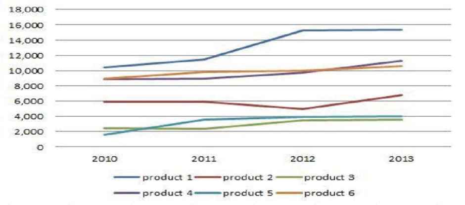
Quantities of products manufactured in period 2010–2013
All products produced by manufacturer are sent to the distributing centre, and there they are classified and uploaded in a certain number of vehicles. Afterwards, products are sent to consumer centres according to their demands. In this model we consider a network of 10 potential consumer centres. At the end of life cycle, products are returned by customers to the customer centre and then are sent to a depot for disassembling of returned products, where they are classified into two groups: those that can be repaired and those that cannot be repaired. We consider two potential locations for depots for disassembling. Depending on this classification, products are returned to the manufacturer and re-entered in the production stream, or shipped to the disposal centres. We consider two potential locations for disposal centres. Also, we consider 15 vehicles with capacities varying from 310 to 350 products per vehicle. One of the main activities in reverse logistics flow is transportation of the returned products; this greatly influences economic viability of product recovery (Dat et al., 2012) and this is the main reason why we investigate not only shipping costs, but also fixed transportation costs. Transportation influences environmental pollution, and transportation costs should be reduced to an acceptable level. Otherwise, transport and its costs are in conflict with the motivation of recovering. Therefore, transportation costs take a very significant place in reverse logistics flow.
The aim of our experiment is to find an optimal solution taking into consideration minimization of costs, as presented in the paper. In this model, recovery of products is performed in the manufacturing centre. A simplified network is presented in Fig. 2.
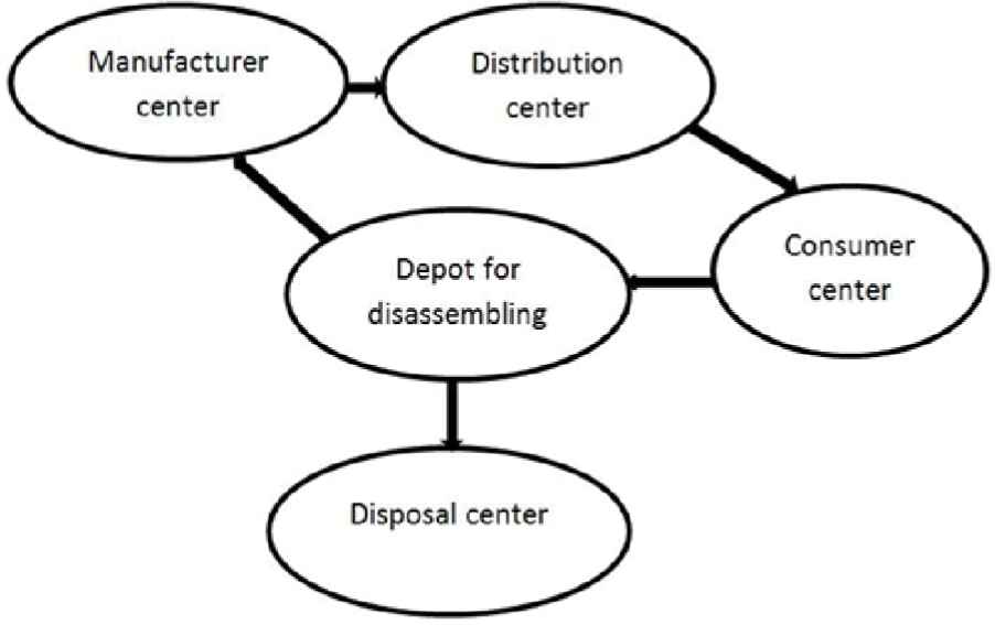
Network model of IFRL
Facility opening costs are investments needed to open a new facility. Opening costs are not investigated for consumer centres. Shipping costs are considered for all vehicles that go from one node to another and they are presented as unit costs. Operation costs include costs of performing different types of operations in all facilities, as follows:
- •
Manufacturing centres – production costs
- •
Distribution centres – repackaging costs
- •
Customer centres – sales and collection costs
- •
Depots for disassembling – disassembling costs
- •
Disposal centres – costs of destruction of the products or parts of the products that have reached their end of life
Integrated forward and reverse model presented in this paper takes into consideration potential penalty costs that could occur if products are not delivered on time.
4. Model development
The assumptions:
- •
All orders are delivered by the supplier to the manufacturer.
- •
There are several kinds of product.
- •
Penalties apply only in the case when customer demands are not satisfied in total.
- •
The capacity of all facilities except manufacturing centres is known in advance.
- •
Manufacturing centres and suppliers are uncapacitated.
- •
The capacities of vehicles are known in advance.
- •
The percentage of collected products is known in advance.
4.1. Notation
Parameters, decision variables, objective function and restrictions in integrated forward and reverse logistics model are as follows:
- P
– set of products p = 1…P
- I
– set of potential locations for manufacturing centre that produces or repairs products i = 1…I
- J
– set of potential locations for distribution centres in which new products are shipped from the plants j = 1…J
- K
- set of potential locations for customer centre k = 1…K
- L
– set of potential locations for depot where products delivered from the consumer k are classified into those that can be repaired and those that cannot be repaired l = 1…L
- M
– set of potential disposal centres with delivered products and parts of products that cannot be repaired or reused m = 1…M
- U
– set of vehicles u = 1…U
- dkp
– demand of consumer k for product p
- y
– the percentage of products that are removed from further use
- r
– the percentage of products that have to be disposed of
- fi
– fixed cost of opening manufacturing centre i
- gj
– fixed cost of opening distribution centre j
- al
– fixed cost of opening depot for returned products l
- bm
– fixed cost of opening disposal centre m
- vu
– fixed cost of vehicle using u
– shipping cost per unit of product p from distribution centre j to customer k
– Shipping cost per unit of product p from customer k to depot l
– Shipping cost per unit of product p from depot l to manufacturing centre i
– Shipping cost per unit of product p from depot l to disposal centre m
– penalty cost per unit of product p of non-satisfied demand of customer centre k
- ϕip
– manufacturing/recovering cost per unit of product p in manufacturing centre i
- φjp
– processing cost per unit of product p in distribution centre j
- γkp
– processing cost per unit of product p in customer centre k
- ηlp
– classification cost per unit of product p in depot l
- μmp
– disposal cost per unit of product p in disposal centre m
- ck1
- capacity of customer center k
- cm2
- capacity of disposal center m
- Nj1
– maximal flow through distribution centre j
- Nl2
– maximal flow through depot l
- qv
- capacity of vehicle
- A
– large number
- Xijp1
– quantity of product p shipped from manufacturing centre i to distribution centre j
- Xjkp2
– quantity of product p shipped from distribution centre j to customer centre k
- Xklp3
– quantity of product p shipped from customer centre k to depot l
- Xlip4
– quantity of product p shipped from depot l to manufacturing centre i
- Xlmp5
– quantity of product p shipped from depot l to disposal centre m
- βkp
– quantity of non-satisfied demand of customer k for product p
- Wi
– indicator of manufacturing centre location, Wi = 1, if manufacturing centre is opened at location i, Wi = 0 otherwise
- Sj
– indicator of distribution centre location, Sj = 1, if distribution centre is opened at location j, Sj = 0 otherwise
- Ll
– indicator of depot location, Ll = 1 if depot is opened at location l, Ll = 0 otherwise
- Vm
– indicator of disposal centre’s location, Vm = 1, if disposal centre is opened at location m, Vm = 0 otherwise
– indicator of distribution centre’s supplier,
– indicator of consumer centres supplier,
– indicator of depots supplier,
– indicator of manufacturing centre’s supplier,
– indicator of disposal centre’s supplier,
4.2. Mathematical model
The objective function contains four parts:
The mathematical problem is to minimize:
The first part of objective function (1) presents the total opening costs of manufacturing centres, distribution centres, depots and disposal centres. The second part of objective function (2) presents the total shipment costs and costs of performing operations in manufacturing centres, distribution centres, consumer centres, depots and disposal centres. The third part of objective function (3) presents fixed cost of vehicles (amortization costs, taxes, etc.). The fourth part of objective function (4) presents total penalty costs. The objective function (5) minimizes total costs. Constraint (6) explains that all customers’ demands are not satisfied. Constraint (7) presents returned products that are collected from all customers. Constraints (8), (9) and (10) ensure that there are flow balances between manufacturing centres and distribution centres, consumers and depots, and depots and disposal centres, respectively. Constraints (11) and (12) present capacity constraints for consumer and disposal centres, while constraints (13) and (14) present capacity constraints for distribution centres and depots. Constraint (15) ensures that quantity of products that are returned cannot be greater than quantity of products that are delivered. Constraints (16) – (20) present capacity constraints for vehicles. Constraint (21) presents capacity restriction for manufacturing centre. Constraint (22) presents binary restriction for listed decision variables. Constraint (23) presents a binary restriction for the quantities.
5. Computational results
In this section, at first we present input data and computational results for test examples. We present several numerical examples in order to evaluate the performance of IFRL model. Data collection for building up the mathematical IFRL model is performed in cooperation with the company which produces electrical and electronic equipment. Detailed input data for case study are collected by interviewing decision-makers in the company. Finally, the verification of mathematical model and sensitivity analysis are presented. All interested readers can obtain the data set and CPLEX code for real case study from the authors. The running time is presented for an AMD triple core processor 2.10 GHz. Parameters of test problem, for which dimensions are [2 2 2 3 1 1 2], are presented in Table 1.
| Data for test problem 1 | ||||
|---|---|---|---|---|
| P=2 | y=50% | qv=30,35 | ckp9=6,8,4 for p1 | cklp3=2,2,5 for l1,p1 |
| I=2 | r=10% | dk1=2,4 for p1 | ckp9=9,7,4 for p2 | cklp3=3,3,8 for l1,p2 |
| J=2 | fi=3,5 | dk2=2,1,7 for p2 | cijp1=2,4 for j1, p1 | clip4=2 for i1, p1 |
| K=3 | gj=2,4 | ϕip=1,2 for p1 | cijp1=4,5 for j2, p1 | clip4=7 for i2, p1 |
| L=1 | ai=4 | ϕip=4,3 for p2 | cijp1=5,7 for j1, p2 | clip4=3 for i1, p2 |
| M=1 | bm=4 | φjp=3,6 for p1 | cijp1=7,8 for j2, p2 | clip4=8 for i2, p2 |
| U=2 | vu=1,2 | φjp=4,8 for p2 | cjkp2=1,8 for k1, p1 | clmp5=3 for m1,p1 |
| ck1=15,20,25 | γkp=7,5,1 for p1 | cjkp2=2,5 for k2, p1 | clmp5=6 for m1,p2 | |
| cm2=50 | γkp=5,5,9 for p2 | cjkp2=3,2 for k3, p1 | ||
| Nj1=25 | ηlp=2,3 | cjkp2=8,9 for k1, p2 | ||
| Nl2=40 | μmp=2,4 | cjkp2=7,8 for k2, p2 | ||
| cjkp2=3,8 for k3, p2 | ||||
Data set for test problems
Apart from test problem with dimensions [2 2 2 3 1 1 2], we performed two more test problems. Input parameters for these problems are not presented. They are performed in order to evaluate the proposed model. Optimal solutions of all test problems are reported in Table 2.
| Problem size | CPLEX | |
|---|---|---|
| P * I * J * K * L * M * U | f(x) | CPU |
| 2 * 2 * 2 * 3 * 1 * 1 * 2 | 208.48 | 0.06 |
| 3 * 2 * 3 * 4 * 2 * 1 * 2 | 497.98 | 0.22 |
| 4 * 4 * 3 * 5 * 2 * 2 * 5 | 862.27 | 1.89 |
f(x) for test instances
Problem is solved for real data. Real input data are presented in Table 3. Value of objective function is 3,052,434.27 monetary units. We will consider this result as case base for the sensitivity analyses that will be performed in the following section.
| The values of the parameters used for real problem | |||
|---|---|---|---|
| P=6 | fi=uniform (300,000; 400,000) | qv=uniform (300,350) | ckp9=uniform (2,5) |
| I=6 | gj=uniform (200,000; 400,000) | dkp=uniform (100,700) | cijp1=uniform (3,5) |
| J=6 | al=uniform (300,000; 400,000) | ϕip=uniform (30,60) | cjkp2=uniform (3,5) |
| K=10 | bm=uniform (250,000; 300,000) | φjp=uniform (10,20) | cklp3=uniform (3,5) |
| L=5 | vu=uniform (10;20) | γkp=uniform (10,15) | clip4=uniform (3,5) |
| M=5 | ck1=uniform (1,000; 2,500) | ηlp=uniform (5,8) | clmp5=uniform (3,5) |
| U=15 | cm2=uniform (4,000; 5,000) | μmp=uniform (3,6) | |
| y=20% | Nj1=uniform (2,000; 2,500) | ||
| r=10% | Nl2=uniform (3,000; 3,000) | ||
The values of the parameters used for real problem
5.1. Sensitivity analyses
The method used for sensitivity analyses is ‘One-at-atime (OAT)’ method. Because of its simplicity, it is one of the most commonly used methods. It is based on the changing of one parameter at a time, while all other parameters have their baseline values. In this paper, OAT method is used in order to evaluate how total costs are changeable regarding the modification in uncertain parameters.
There are several parameters with uncertain values in practice. To illustrate the applicability of the proposed model, we considered percentage of the products that are removed from further use and percentage of disposed products as uncertain values. Values of all other parameters are presented in Table 3.
Table 4 presents results for 21 tests with variable percentages of products removed from further use and percentages of products that are disposed of. Prediction of the experts and decision-makers is that percentage of products that are removed from further use can vary from 10% up to 35%, and thus percentages of the products that are delivered to the disposal centre vary from 5% up to 15% of total number of products, as presented in Table 4.
| y | r | CPLEX | CPU |
|---|---|---|---|
| 10.00% | 5.00% | 2,709,851.75 | 539.29 |
| 12.50% | 5.00% | 2,709,872.03 | 628.63 |
| 10.00% | 3,052,139.06 | 5,741.54 | |
| 15.00% | 5.00% | 2,709,939.07 | 6,847.36 |
| 10.00% | 3,052,245.78 | 6,075.12 | |
| 12.50% | 3,099,757.30 | 6,258.97 | |
| 17.50% | 5.00% | 2,710,001.67 | 810.72 |
| 10.00% | 3,052,258.22 | 2,149.92 | |
| 15.00% | 3,132,203.30 | 6,958.92 | |
| 20.00% | 5.00% | 2,710,026.58 | 7,984.45 |
| 10.00% | 3,052,434.27 | 1,151.34 | |
| 15.00% | 3,132,443.76 | 7,845.45 | |
| 25.00% | 5.00% | 2,710,066.06 | 4,151.23 |
| 10.00% | 3,052,610.10 | 4,781.56 | |
| 15.00% | 3,132,688.53 | 6,377.13 | |
| 30.00% | 5.00% | 2,710,133.88 | 6,587.14 |
| 10.00% | 3,052,675.51 | 381.65 | |
| 15.00% | 3,132,798.90 | 11,461.83 | |
| 35.00% | 5.00% | 2,710,282.57 | 3,458.12 |
| 10.00% | 3,052,771.35 | 6,152.22 | |
| 15.00% | 3,133,050.84 | 7,825.32 | |
Sensitivity analyses results
Optimal value for objective function varies from 2,709,851.75 up to 3,133,050.84 monetary units with different percentage of returned and disposed of product Value gap is calculated as the difference between objective function values for the same percentage of the product that are removed from further use, and different percentage of the disposed of products.
Then we calculated value gap (Table 5).
| y | 12.50% | 15.00% | 17.50% | 20.00% |
|---|---|---|---|---|
| r=5–10% | 342,267 | 342,306 | 342,256 | 342,407 |
| r=10–15% | / | / | 80,345 | 80,009 |
| y | 25.00% | 30.00% | 35.00% | Average |
| r=5–10% | 342,544 | 342,541 | 342,488 | 342,401 |
| r=10–15% | 80,078 | 80,123 | 80,279 | 80,167 |
Value gap
Finally, average values for gap are calculated. Average value is calculated as arithmetic mean of all values for gap. Increment of the percentage of the disposed of products from 5% to 10%, causes the increment of the total costs for average gap of 342,401.78 monetary units. This means that one more disposal centre should be opened if percentage of the disposed products is 10%. However, increment of the percentage of the disposed of products from 10% to 15% does not cause the need to increment the number of disposal centres.
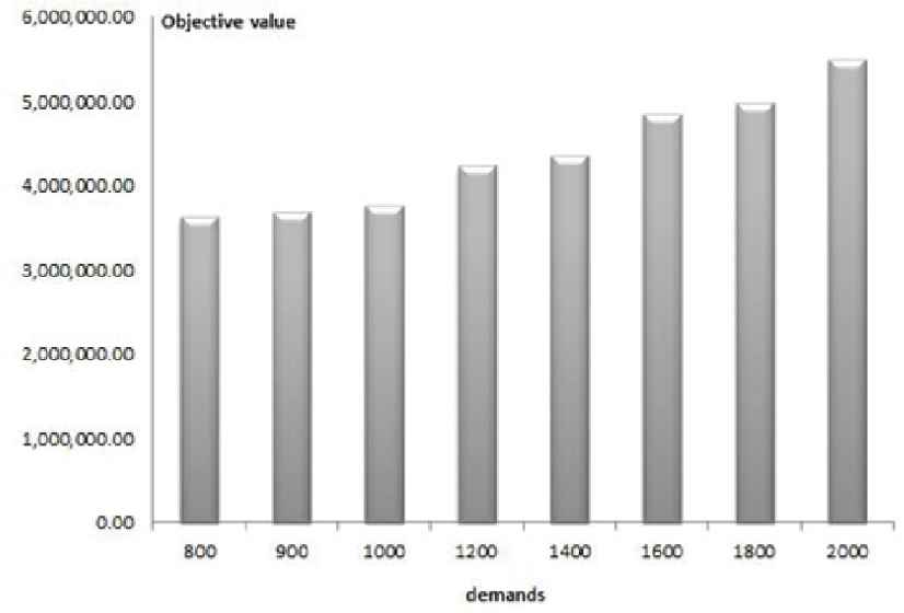
Also, we present sensitivity analyses based on different values of consumer demands. In the first part of the analyses, consumer demands are estimated between 100 and 700 for one consumer centre and one product. In this part of the analyses, we calculate the value of objective function if consumer demand increases. Increment of consumer demands vary from 800 up to 2,000. It is assumed that demands for all products and all consumer centres are the same.
Objective function values for different consumer demands are presented in Fig. 3. All other data are as presented in Table 3.
Objective values for different demands
Objective function values vary from 3,633,618.04 up to 5,495,600.55 monetary units. Results of sensitivity analysis show that the objective function value for presented IFRL is very sensitive to changes in demand. Planning for an increase in demand would result in a network that has higher total costs than the base case, as shown in Table 6.
| Demand | Difference to the case base (%) |
|---|---|
| 800 | 15.99% |
| 900 | 17.40% |
| 1000 | 18.79% |
| 1200 | 27.99% |
| 1400 | 30.06% |
| 1600 | 37.23% |
| 1800 | 38.80% |
| 2000 | 44.46% |
Sensitivity analysis for different demands
6. Conclusion
Modern business conditions are characterized by limited resources and capacities of facilities for waste disposal. Thus, repair and re-use of already used products and materials are important in order to support a growing population and increasing levels of consumption and usage of the products. Adequate design of logistics network provides an appropriate platform for efficient and effective supply chain management. The problem solved in this paper refer to the determination of integrated logistics network in one Serbian company. The purpose of the research was to unite the network of logistics and reverse logistics supply, due to its contribution on the efficiency and effectiveness of the entire supply chain. We presented original integrated forward and reverse logistics mathematical model in this paper. Integration of forward and reverse logistic is not implemented in large number of papers. The contribution of the paper was to develop model which supports reuse of electrical and electronic equipment. IFRL model takes into account costs and investments for opening of new facilities in forward and reverse flow, as well as shipping and processing costs in all facilities in forward and reverse flow. Decision-makers and experts took into account penalty costs that could occur if products are not delivered. In order to solve the presented model we used real instances gathered from a company that produces large and small household devices, and model is solved using CPLEX solver. Two different sensitivity analyses are presented.
Development of reverse logistics flow and adopting of the idea of sustainable development is, also, very important on a national level, especially taking into consideration the position of Serbia, which strives for integration with the European Union. Similar models could be developed and solved for the disposal and waste landfill locations on the national level.
For future research the usage of other methods for the evaluation of validity of proposed model and work could be considered. A limitation of the proposed model is that for large problems, CPU time can be unduly long, and usage of heuristics research is proposed for problems with larger instances.
References
Cite this article
TY  - JOUR
AU  - Jasenka Djikanovic
AU  - Mirko Vujosevic
PY  - 2016
DA  - 2016/01/01
TI  - A new integrated forward and reverse logistics model: A case study
JO  - International Journal of Computational Intelligence Systems
SP  - 25
EP  - 35
VL  - 9
IS  - 1
SN  - 1875-6883
UR  - https://doi.org/10.1080/18756891.2016.1144151
DO  - 10.1080/18756891.2016.1144151
ID  - Djikanovic2016
ER  -