1. Introduction

Multiple criteria decision analysis (MCDA) denotes to analyzing decision making situations that encounter with multiple and conflicting criteria. It refers to analyzing tools and systematic approaches that empower the decision maker (DM). They help DM to represent his/her preferences and consider all subjective and objective conditions to assess the decision elements [1, 2]. MCDA methods provide a quantitative infrastructure to model the assessments of criteria and alternatives [3]. MCDA methods are classified into three major categories including multi-attribute value theory (MAVT), multi-objective mathematical programming, and outranking methods [4, 5, 6, 7, 8, 9].

(1) MAVT approach concerns hierarchical decision making problems with the overall goal on the top level and the criteria on the lowest level. MAVT involves in the weighting the criteria and assessment of alternatives with respect to criteria. Lastly, MAVT approach ranks the criteria through calculations of criteria weights and alternative assessments.

(2) Multi-objective mathematical programming methods focus on finding the aspiration points. These points can generate non-dominated solutions by scalarizing functions through reaching down from ideal solution [10, 11, 12].

(3) Outranking methods form two main steps: building the outranking relations, and exploiting the outranking relations [13]. At first, outranking methods systematically compare criteria. The binary comparisons construct the concordance and discordance sets which are linguistic comparisons. Then, these comparisons lead to numerical concordance and discordance indices.

There are different outranking methods including ELECTRE family, PROMETHEE family, QUALIFLES [14], ORESTE [15, 16], MELCHIOR [17], PRAGMA [18], MAPPACC [18], and TACTIC [19]. ELECTRE family includes ELECTRE I [20, 21], ELECTRE II [22, 23], ELECTRE III [24, 25], ELECTRE IV [26], ELECTRE IS [27], ELECTRE TRI [28], and ELECTRE^GKMS [29]. PROMETHEE family contains PROMETHEE I [30], and PROMETHEE II [30].

The PROMETHEE family of outranking methods includes the PROMETHEE I for partial ranking of the alternatives and the PROMETHEE II for complete ranking of the alternatives, the PROMETHEE III for ranking based on interval, the PROMETHEE IV for complete or partial ranking of the alternatives when the set of viable solutions is continuous, the PROMETHEE V for problems with segmentation constraints, the PROMETHEE VI for the human brain representation [31].

ELECTRE family methods are the most widely used outranking approaches [29, 32]. ELECTRE I outranking method is the first ELECTRE method which was introduced by Benayoun, Roy, and Sussman [20] and Roy [21]. Decision makers use ELECTRE I to construct a partial prioritization and choose a set of promising alternatives [4]. ELECTRE II is used for ranking the alternatives based on the determination of concordance and discordance matrices for each criterion and alternative pair. In ELECTRE III, an outranking degree is established, representing an outranking creditability between two alternatives which makes this method more sophisticated. ELECTRE III is based on the principle of fuzzy logic and uses the preference and indifference thresholds while determining the concordance and discordance indices [13].

Outranking methods are extended to deal with imprecision and uncertainty of decision making process. Roy [33] and Siskos, Lochard, and Lombard [34] developed fuzzy outranking method. This method uses fuzzy concordance and discordance relation. Sevkli [35] applied fuzzy ELECTRE method for supplier selection. Ertay and Kahraman [36] evaluated the design requirements by utilizing fuzzy outranking methods.

Afterwards, different extensions of fuzzy sets have been applied to outranking methods. Interval type-2 fuzzy sets have been employed in the ELECTRE method [37, 38]. Chen [39] implemented an ELECTRE based group decision making method using interval type-2 fuzzy sets. Devi and Yadav [40] developed an ELECTRE group decision making based on intuitionistic fuzzy sets for plant location selection. See Vahdani et al. [41], Li, Lin, and Chen [42], and Wue and Chen [43] developed ELECTRE method extension in an intuitionistic fuzzy environment. Hatami-Marbini and Tavana [4] applied fuzzy group decision making to extend ELECTRE I methodology. See Hatami-Marbini and Tavana [4] for more details.

Torra [44] proposed hesitant fuzzy sets (HFS) as a generalization of fuzzy sets. HFS are quite suitable in decision making when experts have to assess a set of alternatives. HFS were introduced to the literature for the common difficulty that often appears when the membership degree of an element must be established and the difficulty is not because of an error margin (as in intuitionistic fuzzy sets) or due to some possibility distribution (as in type-2 fuzzy sets), but rather because there are some possible values that cause hesitancy about which one would be the right one [45].

These new sets permit DM to represent his/her hesitation in decision making process. The mathematical background of hesitation is modeled by different membership functions. HFS establishes a relationship between the envelopes of fuzzy sets and generates new fuzzy sets with combined membership functions.

As decision making encounters linguistic information, we need to use computing with words (CWW) processes [46, 47, 48]. HFS provides an appropriate infrastructure to develop the concept of hesitant linguistic term set which is a useful CWW process. The experts involved in decision problems under uncertainty cannot easily provide a single term as an expression of his/her knowledge such as poor, good, very good, etc. because they might consider several terms at the same time or looking for a more complex linguistic term such as at least medium poor, at most very high, etc. Thus, Rodriguez, Martinez, and Herrara [49], and Liu and Rodriguez [50] proposed the hesitant fuzzy linguistic term set (HFLTS) and its application in decision making. This method could increase the ability and flexibility of linguistic elicitation of DM. HFLTS enables DM to represent the uncertainty in his/her assessments of actions, criteria, alternatives, etc. [49]. This would be implemented by context-free grammars based on the fuzzy linguistic tools to compare the expressions.

In this study, the ELECTRE I method is extended based on HFLTS. This new approach could be applied to decision making problems and deal with the uncertainty and imprecision of multiple criteria decision making. This method contains two phases: HFLTS phase and ELECTRE I phase. Firstly, HFLTS method considers DM’s hesitation between several values to evaluate the decision elements and manage the uncertainty of decision making. These hesitant linguistic terms are expressed by numerical fuzzy values. Next, in ELECTRE phase, we apply ELECTRE I method to analyze the decision making. This would be accomplished through building the outranking relations, and then exploiting the outranking relations. Finally, we can rank the alternatives and make an appropriate decision.

It is worthy to mention that ELECTRE method has an important pitfall [4]. DM must initiate this method by precise measurement of the performance ratings and the weights of criteria [5]. On the other hand, DM may prefer to express his/her judgment by linguistic expressions [51, 52, 53]. This approach takes this weakness into account and modifies it by utilizing linguistic expressions in decision making process and allows DM to evaluate the real world problem with imprecise and vague ratings.

This paper is organized as follows: Section 2 includes needed definitions and arithmetic operations about HFLTS and ELECTRE I method. In Section 3, the step-by-step methodology of hesitant fuzzy linguistic term set ELECTRE I (HFLTS-ELECTRE I) is proposed. Next, a real case study is added in Section 4. Lastly, the conclusions and future works are presented in Section 5.

2. Preliminaries

In this section, the basic definitions and arithmetic operations are given.

2.2. Fuzzy arithmetic operations

Based on the previous definitions, proposed method employs trapezoidal fuzzy numbers and arithmetic operations of trapezoidal fuzzy numbers should be calculated. The required concepts are defined below.

Definition 6.

A fuzzy number à = (a,b,c,d) is a trapezoidal fuzzy number shown in Fig. 1, and its membership function is given by:

(8)μ(x)={0,x<a,x−ab−a,a≤x≤b,1,b<x<c,d−xd−c,c≤x≤d,0,x>d,

Fig. 1.

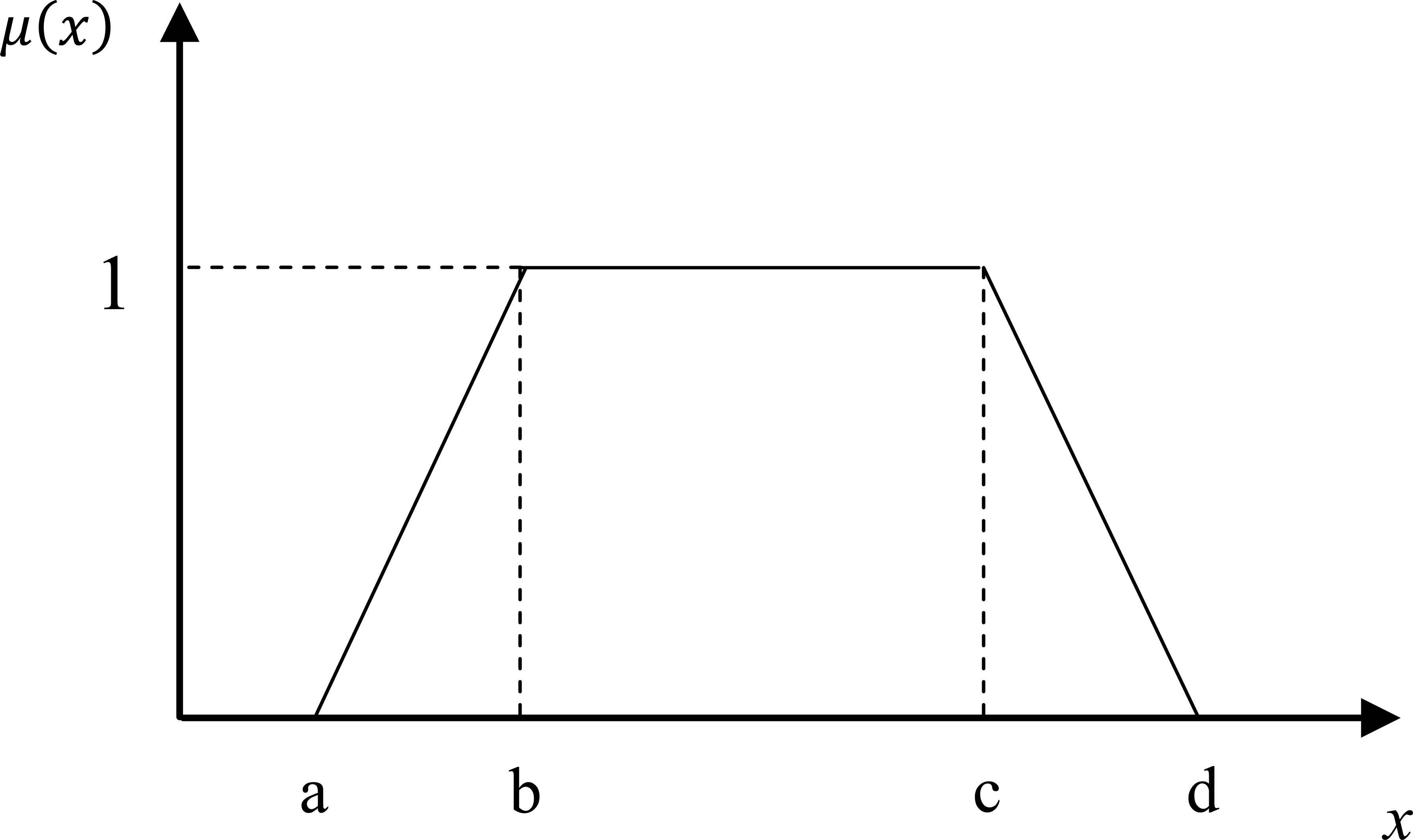
Trapezoidal fuzzy number, Ã = (a,b,c,d)

Definition 7.

Let A and B be two positive trapezoidal fuzzy numbers, where à = (a,b,c,d) and B˜=(p,q,r,s) . The arithmetic operations between à and B˜ is as follows:

• Addition operation:

  (9)A˜⊕B˜=(a+p,b+q,c+r,d+s)

• Subtraction operation:

  (10)A˜⊖B˜=(a−s,b−r,c−q,d−p)

• Multiplication operation:

  (11)A˜⊗B˜≅(ap,bq,cr,ds)

• Division operation:

  (12)A˜⊘B˜≅(as,br,cq,dp)

• Multiplication operation:

  (13)u.A˜=A˜.u={(u·a,u·b,u·c,u·d)if u≥0(u·d,u·c,u·b,u·a)if u<0

• Division operation:

  (14)A˜u={(au,bu,cu,du)if u≥0(du,cu,bu,au)if u≤0

3. Methodology

As mentioned above, we propose a new fuzzy ELECTRE I method based on HFLTS. This method facilitates decision making process due to utilizing linguistic terms and context-free grammars for evaluating the importance weights of the criteria and performance ratings. Since DMs compare the criteria and alternatives to present relative assessments, comparative linguistic expressions are needed for the assessments of alternatives and criteria. Therefore, HFLTS method contributes to determine fuzzy numbers for hesitant judgments. Then, fuzzy ELECTRE I outranking method is established to complete the decision making process. Our methodology includes two main phases: HFLTS operations and the application of fuzzy ELECTRE I outranking method.

I. First phase: HFLTS operations

Step 1. Determine the semantics and syntax of linguistic terms set and context-free grammar G_H.

In this phase, DM should determine the decision making conditions to apply CWW process. The first step is to determine the semantic and syntax of comparative linguistic terms set. Definition 1 also lets us to determine the context-free grammar G_H. An example of context-free grammar is provided below [50]:

GH={VN,VT,I,P}

where V_N shows non-terminal symbols and V_T shows terminal symbols as follows:

VN={〈primary term〉,〈binary relation〉, 〈unary term〉,〈conjunction〉}VT={at least, at most, between, and, S0, S1,…,Sg}I∈VN

P indicates the production rules for the context-free grammar G_H. Bracket signs shows optimal elements and the symbol “|” indicates alternative elements. In this example, the production rules are as follows:

P={primary term::=s0|s1|…|sg,〈binary relation〉::=between,〈unary relation〉::=at least|at most|lower than|greater than,〈conjunction〉::=and}

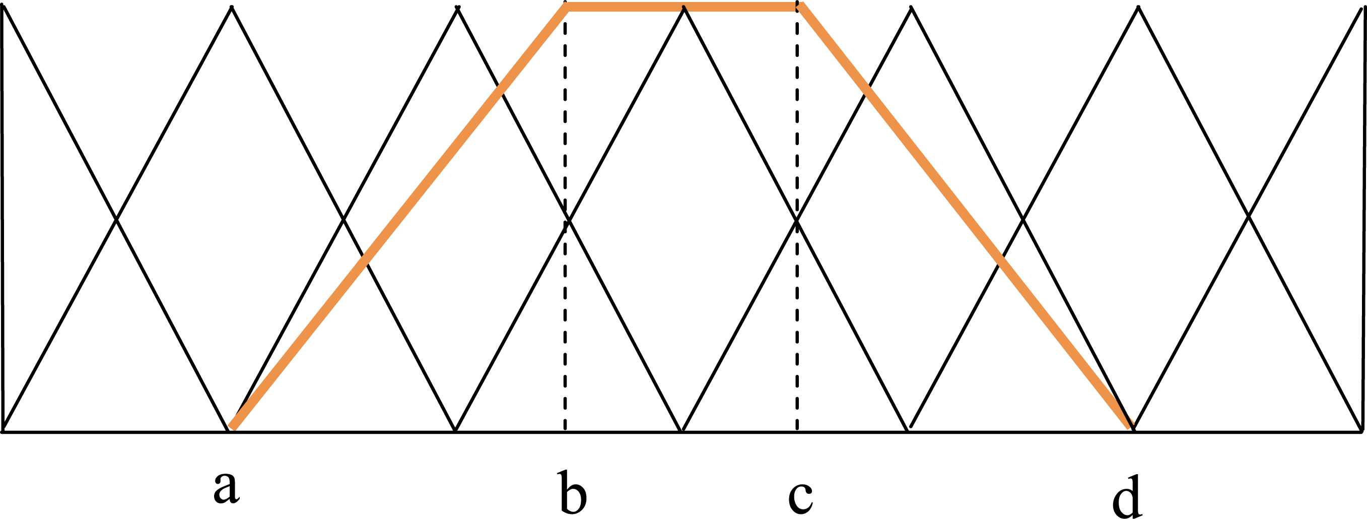
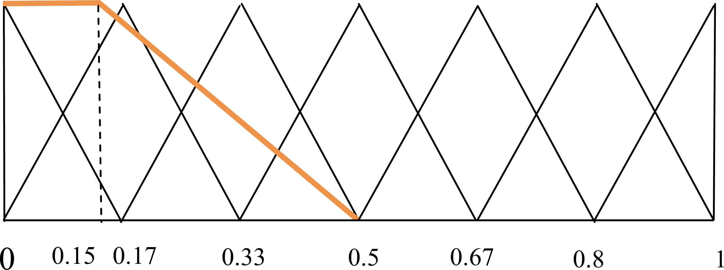
This set specifies the fuzzy partition of the HFLTS phase. This partitioning lets us to represent the fuzzy envelopes of the assessments. Three values are considered including left value (L), middle value (M), and right value (R) for the partitioning. As you see in Fig. 2, each triangular represents three values L, M, and R. In the proposed approach, assessments are represented by trapezoidal fuzzy numbers.

Fig. 2.

Fuzzy partitioning.

Step 2. Gather the assessments of performance and criteria.

In this step, DM evaluates the performance ratings with respect to criteria in square matrices. Also, the weights of criteria are calculated by DM’s assessments of criteria with respect to goal.

Step 3. Transform the assessments into HFLTS by transformation function E_GH.

Let S = {s₀,s₁,…,s_g} be the linguistic terms set. DM evaluates the performance and criteria by comparative linguistic terms based on the defined context-free grammar G_H. The transformation of the evaluations into HFLTS will be carried out by transformation function E_GH as follows:

EGH(si)={si|si∈S}={si},EGH(between si and sj)={sk|si≤sk≤sj and sk∈S}={si,si+1,…,sj},EGH(at least si)={sj|sj≥si and sj∈S}={si,si+1,…,sg}, EGH(at most si)={sj|sj≤si and sj∈S}     ={s0,s1,…,si}

Step 4 : Obtain an aggregate set for each assessment.

In this step, the fuzzy envelope is obtained through calculating the elements of a trapezoidal fuzzy number. We calculate these elements by aggregate set as follows: Let A be the aggregate set for E_GH (between s_i and s_j)

(15)Abetween={aLi,aMi,aLi+1,aRi,aMi+1,aLi+2,aRi+1,…,aLj,aRj−1,aMj,aRj}

(16)Aat least={aLi,aMi,aLi+1,aRi,aMi+1,aLi+2,aRi+1,…,aLg,aRg−1,aMg,aRg}

(17)Aat most={aL0,aM0,aL1,aR0,aM1,aL2,aR1,…,aLi,aRi−1,aMi,aRi}

As you see in Fig. 2, aLk+1=aMk=aRk−1 for k = 1,2, …,g − 1. So that, the Eqs. (15), (16), and (17) are simplified as follows:

Abetween={aLi,aMi,aMi+1,…,aMj,aRj}Aat least={aLi,aMi,aMi+1,…,aMg,aRg}Aat most={aL0,aM0,aM1,…,aMi,aRi}

Step 5. Obtain fuzzy envelope for each assessment.

T˜between=(a,b,c,d),

a

= min Abetween=min{aLi,aMi,aMi+1,…,aMj,aRj}=aLi ,

d

= max Abetween=max{aLi,aMi,aMi+1,…,aMj,aRj}=aRj ,

b

= OWAW2(aMi,aMi+1,…,aMj) ,

c

= OWAW1(aMi,aMi+1,…,aMj) .

As in Definition 5, we can compute the weights of OWA operator to calculate element b, and c for “between” comparative linguistic terms set. The first type of weights of OWA operator is used to calculate b and the second type of weights of OWA operator to calculate c as follows:

1. I)

   If i+j is odd, then

   b=OWAW2(aMi,aMi+1,…,aMi+j−12),c=OWAW1(aMj,aMj−1,…,aMi+j+12),W2=(w12,w22,…,wj−i+1/22)T and α1=g−(j−i)g−1

   where

   w12=α1j−i−12,w22   =(1−α1)α1j−i−32,…,wj−i−122=(1−α1)α1,wj−i+122=(1−α1)b=w12·aMi+j−12,w22·aMi+j−32,…,wj−i−122·aMi+1,wj−i+122·aMi

   and W1=(w11,w21,…,wj−i+1/21)T and α2=1−α1=(j−i)−1g−1

   where

   w11=α2,w21=α2(1−α2),…,wj−i−122   =α2(1−α2)j−i−32,wj−i+122=(1−α2)j−i−12c=w11·aMi+j+12,w21·aMi+j−12,…,wj−i−121·aMi+1,wj−i+121·aMi

2. II)

   If i+j is even, then

   b=OWAW2(aMi,aMi+1,…,aMi+j2),c=OWAW1(aMj,aMj−1,…,aMi+j2),W2=(w12,w22,…,wj−i+2/22)T

   where

   w12=α1j−i2,w22=(1−α1)α1j−i−22,…,wj−i22b=w12·aMi+j2,w22·aMi+j−22,…,wj−i22·aMi+1,wj−i+222·aMi

   and W1=(w11,w21,…,wj−i+2/21)T where

   w11=α2,w21=α2(1−α2),…,wj−i21=α2(1−α2)j−i−22,wj−i+221=(1−α2)j−i2 c=w11·aMi+j2,w21·aMi+j−22,…,wj−i21·aMj−1,wj−i+221·aMj

Finally, the HFLTS envelope will be formed as T˜between=(aLi,b,c,aRj) . See Fig. 3.

Fig. 3.

Fuzzy Envelope for comparative linguistic expression “between”

T˜at least=(a,b,c,d),

a

= min Aat least=min{aLi,aMi,aMi+1,…,aMg,aRg}=aLi ,

d

= max Aat least=max{aLi,aMi,aMi+1,…,aMg,aRg}=aRg

b

= OWAW2(aMi,aMi+1,…,aMg)

c

= OWAW2(aMi,aMi+1,…,aMg)

As can be seen in Definition 5, the weights of OWA operator to compute element b for “at least” comparative linguistic terms set are as follows:

n=g−i+1,W2=(w12,w22,…,wn2)T and α=ig

where

w12=αg−i,w22=(1−α)αg−i−1,…,wg−i2=α(1−α)wg−i+12=1−αb=w12·aMg,w22·aMg−1,…,wg−i2·aMi+1,wg−i+12·aMi,b=αg−i·aMg,(1−α)αg−i−1·aMg−1,…,   α(1−α)·aMi+1,(1−α).aMic=aMg

Finally, the HFLTS envelope is formed as T˜at least=(aLi,b,aMg,aLg) . See Fig. 4.

Fig. 4.

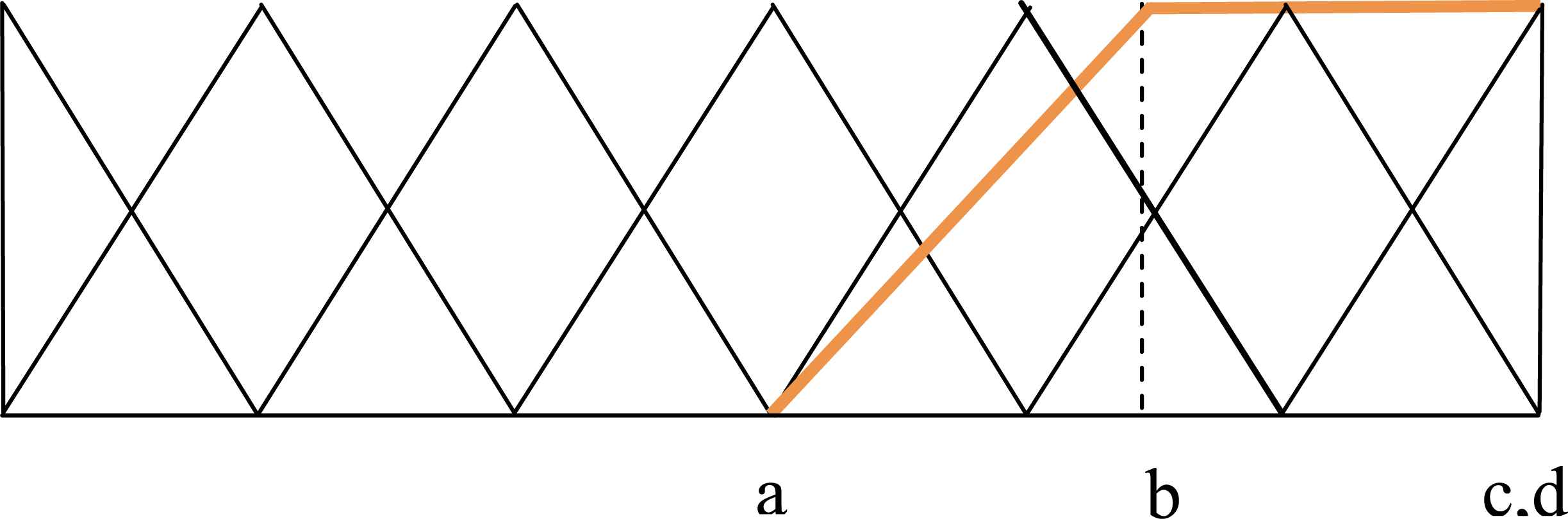
Fuzzy Envelope for comparative linguistic expression “at least”.

T˜at most=(a,b,c,d),

a

= min Aat most=min{aL0,aM0,aM1,…,aMj,aRj}=aL0 ,

d

= max Aat most=max{aL0,aM0,aM1,…,aMj,aRj}=aRj

b

= OWAW1(aM0,aM1,…,aMj)

c

= OWAW1(aM0,aM1,…,aMj)

As you see in Definition 5, the weights of OWA operator to compute element c for “at most” comparative linguistic terms set are as follows:

n=i+1,W1=(w12,w22,…,wn2)T and α=ig

where

w11=α,w21=α(1−α),…,wi1=α(1−α)i−1,wi+11=(1−α)ic=w11·aMi,w21·aMi−1,…,wi1·aM1,wi+11·aM0,c=α·aMi,α(1−α)·aMi−1,…,α(1−α)i−1·aM1,(1−α)i·aM0b=aM0

Finally, the HFLTS envelope is formed as T˜at most=(aL0,aM0,c,aRi) . See Fig. 5.

Fig. 5.

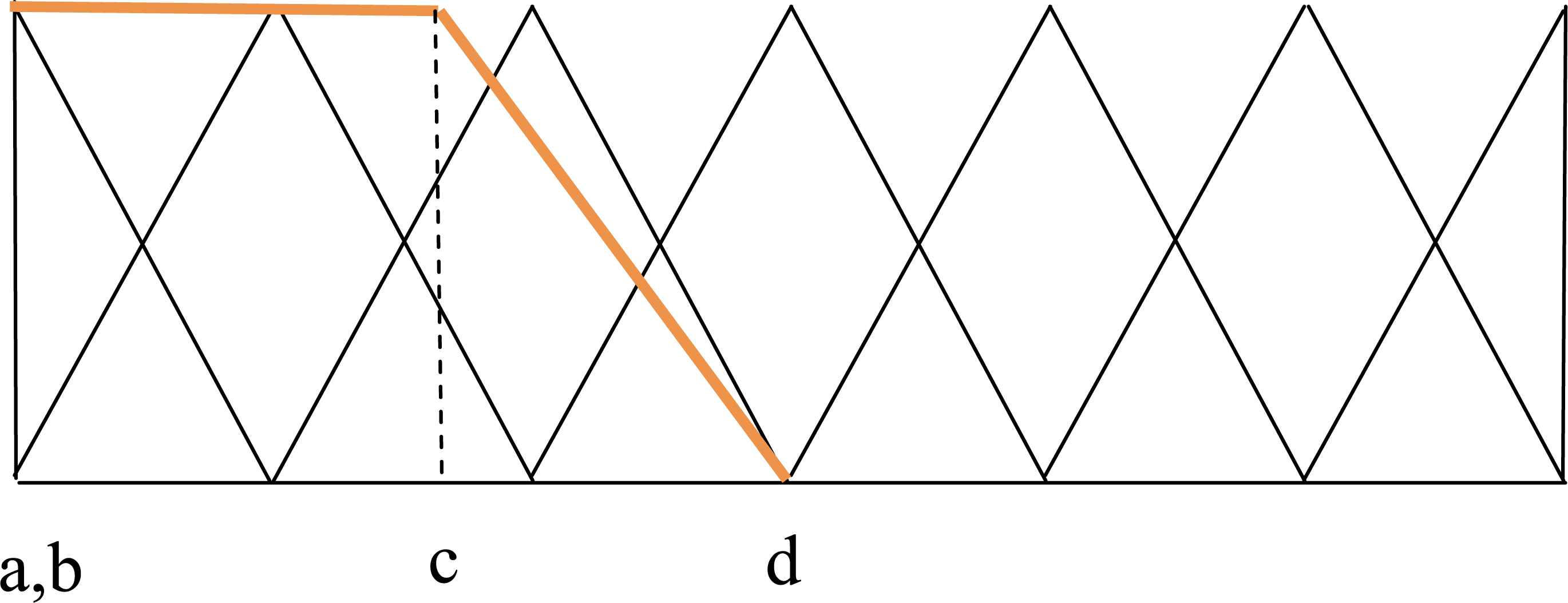
Fuzzy Envelope for comparative linguistic expression “at most”

II. Second phase: ELECTRE I outranking method

Step 6. Defuzzify and rank the alternatives for each criterion.

In this step, the trapezoidal fuzzy values, which DM evaluated the alternatives in previous steps, will be defuzzified. The center of gravity defuzzification method is applied to rank alternatives with respect to each criterion.

Then, the utility matrix Ũ is built. By taking utility matrix into account, assessment matrices will be formed to compare alternatives with respect to each criterion. The trapezoidal fuzzy elements of final utility matrix form the performance ratings as in Eq. (18).

(18)U˜=[−t˜12⋯t˜1nt˜21−⋯t˜2n⋮⋮⋱⋮t˜m1t˜m2⋯−]

The decision matrix Ĩ is also built to compare the importance of criteria. Next, the weight of each criterion could be obtained through computing the average of the elements in each row using summation and division rules of trapezoidal fuzzy numbers. See Definition 7 for more details. Finally, the weight matrix will be obtained as Eq. (20).

(19)I˜=[−F˜12⋯F˜1nF˜21−⋯F˜2n⋮⋮⋱⋮F˜m1F˜m2⋯−]

(20)W˜=[W˜1,W˜2,…,W˜m]T

where W˜1=∑j=2nF˜1jn,  W˜2=∑j=2nF˜2jn , and W˜m=∑j=2nF˜mjn

Since the values in the matrices are between 0 and 1, there is no need to obtain a normalized matrix. The weight matrix W˜ and the utility matrix Ũ are multiplied to construct weighted utility matrix Ṽ as follows:

V˜=[v˜11v˜12⋯v˜1nv˜21v˜22⋯v˜2n⋮⋮⋱⋮v˜m1v˜m2⋯v˜mn]

where

v˜ij

= (vijl,vijp,vijq,viju)=(wjltijl,wjptijp,wjqtijq,wjutiju) ,

i = 1,2, …, m, and j = 1,2, …, n.

Step 7. Calculate the fuzzy concordance indices and discordance indices.

The fuzzy concordance matrix is built as Eq. (21). The elements of this matrix are measured by pairwise comparison of alternatives. In this regard, two alternatives and are considered. Using a_f and a_g are considered. Using Definition 8, the outranking relation a_gSa_gf will be defined. The arguments in favor of this statement “a_f outranks a_g” is measured to obtain the fuzzy concordance indices as follows:

(21)C˜=[−⋯c˜g1⋯c˜1(m−1)c˜1m⋮⋱⋮⋱⋮⋮c˜g1⋯c˜gf⋯c˜g(m−1)c˜gm⋮⋱⋮⋱⋮⋮c˜m1⋯c˜mf⋯c˜m(m−1)−]c˜gf=(cgfl,cgfp,cgfq,cgfu)

where cgfl=∑k:xik≥xjkwklW, cgfp=∑k:xik≥xjkwkpW, cgfq=∑k:xik≥xjkwkqW , and cgfu=∑k:xik≥xjkwkuW and W=∑i=1mw˜i .

In addition, the discordance set is formed to construct the discordance matrix. The concept of discordance set is in contrast to the concept of concordance set. If DM has doubt upon the statement “a_f outranks a_g” and DM is against the assertion “a_g is at least as good as a_f”, we can represent the discordance matrix and the arguments as follows [60]:

(22)D=[−⋯dg1⋯d1(m−1)d1m⋮⋱⋮⋱⋮⋮dg1⋯dgf⋯dg(m−1)dgm⋮⋱⋮⋱⋮⋮dm1⋯dmf⋯dm(m−1)−]

where dgf=∑h°|v˜gh−v˜fh|∑h|v˜gh−v˜fh| , if v˜gh<v˜fh , g = 1,2, …, m, and f = 1,2, …, n, and |v˜gh−v˜fh|=|(vghl−vfhu,vghp−vfhq,vghq−vfhp,vghu−vfhl)| .

The discordance indices are obtained between alternatives i and j with respect to the criterion h°. ṽ_ih and ṽ_jh are ranked by Yager’s centroid index [61]. Then, the defuzzification method, center of gravity will be employed to calculate the discordance index.

Since this method calculates the outranking relations without defining concordance and discordance thresholds, a combination method to unite fuzzy concordance and discordance matrices is proposed. A modified version of Aouam and Chang’s [62] formula is applied to calculate the elements of matrix D′. Hence, D′ is formed by subtracting each element of the discordance matrix from 1. Then, the fuzzy global matrix Z˜ will be calculated through peer to peer multiplication of the elements of the matrices C˜ and D′ (using Eq. (11)) as follows:

(23)Z˜=C˜⊗D′

where

(24)D′=[−⋯1−dg1⋯1−d1(m−1)1−d1m⋮⋱⋮⋱⋮⋮1−dg1⋯1−dgf⋯1−dg(m−1)1−dgm⋮⋱⋮⋱⋮⋮1−dm1⋯1−dmf⋯1−dm(m−1)−]

Step 8. Compare the alternatives by fuzzy Kernel diagram.

In the final step, the outranking relations is exploited to compare the alternatives by the elements of matrix Z˜ . In this regard, graph G = (V,J) is defined, where V is the set of nodes and J is the set of arcs. One node is considered for each alternative and an arc between two nodes of alternatives a_f and a_g. Here, we propose fuzzy Kernel diagram. This diagram could depict uncertainty in comparison of alternatives. We draw solid arc if a_g absolutely outranks a_f, that means a_g is absolutely preferred to a_f as shown in Fig. 6 a. We proposed to draw long dashed arc if a_g strongly outranks a_f as shown in Fig. 6 b, and dashed arc if a_g weakly outranks a_f as shown in Fig. 6 c. If a_g and a_f are incomparable, we consider no arc between them as shown in Fig. 6 d. In addition, Fig. 6 e illustrates the indifference between a_g and a_f.

Fig. 6.

Outranking relations represented by fuzzy Kernel diagram.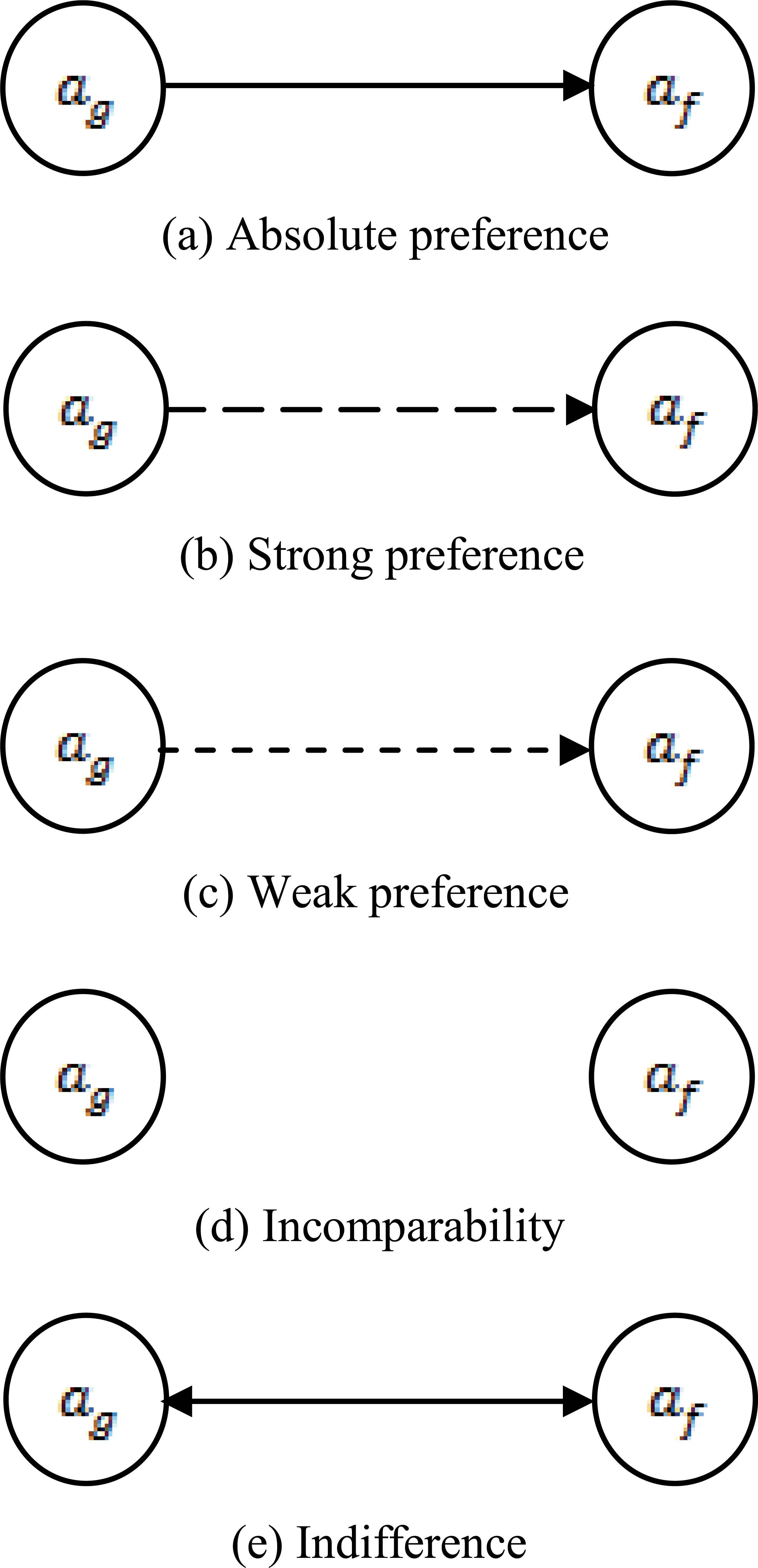

In order to determine the arcs, the elements of fuzzy global matrix Z˜ should be defuzzified. In this step, center of gravity defuzzification method is applied and z_gf represents the defuzzified values. The intervals of the defuzzified values are defined for associated binary preferences are presented below:

(25){Incomparable0≤zgf≤0.25Weak Preference0.25<zgf≤0.5Strong Preference0.5<zgf≤0.75Absolute Preference0.75<zgf≤1

In summary, you can find the associated steps of our combined method as follows:

1. I.

   First phase: HFLTS operations

   • Step 1.

     Determine the semantics and syntax of linguistic terms set and context-free grammar G_H.

   • Step 2.

     Gather the assessments of performance and criteria.

   • Step 3.

     Transform the assessments into HFLTS by transformation function E_GH.

   • Step 4 :

     Obtain aggregate set for each assessment.

   • Step 5.

     Obtain fuzzy envelope for each assessment.

2. II.

   Second phase: ELECTRE I outranking method

   • Step 6.

     Rank alternatives for each criterion.

   • Step 7.

     Calculate fuzzy concordance and discordance indices.

   • Step 8.

     Compare alternatives by fuzzy Kernel diagram.

4. An Illustrative Example

In this part, a simple MCDA problem is added to provide a step by step solution in order to illustrate the proposed method. The problem is the selection of best supplier among three alternatives by considering three attributes including price, quality, and delivery. The best way of illustrating the relations between the criteria and alternatives is to use a hierarchy often applied in Analytic Hierarchy Process (AHP) [63]. The hierarchy of decision making is provided below:

Fig. 7.

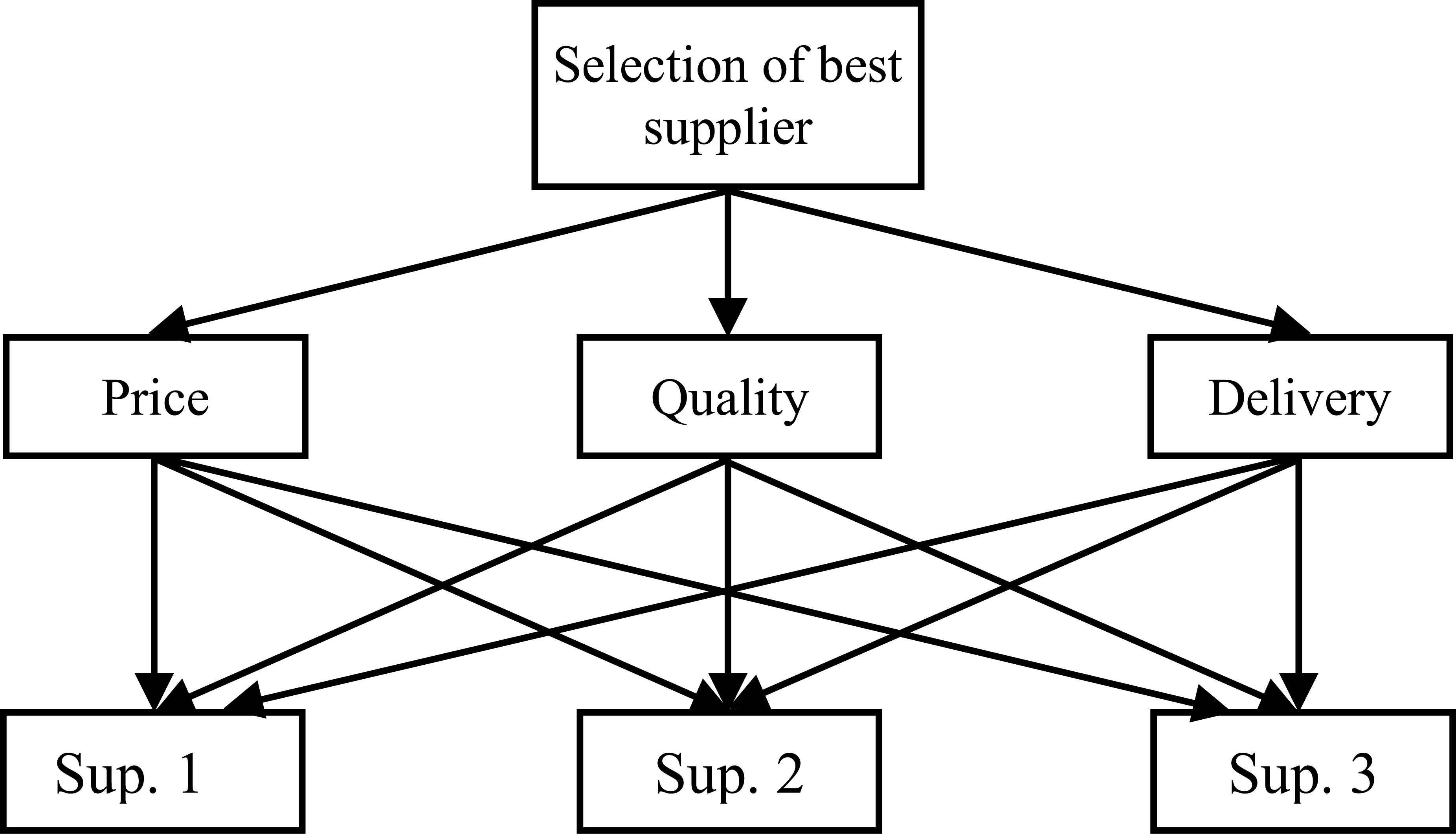
The hierarchy of MCDA supplier selection problem.

The steps of the method are presented below:

Step 1. At first, the semantic and syntax of linguistic term set S and context-free grammar G_H should be defined. We determine the linguistic term set S as:

Step 2. In this step, the importance of criteria is assessed with respect to the goal as Table 1. This will obtain the weights of criteria in next steps. Then, the performance of alternatives with respect to each criterion will be evaluated as you see in Tables 2, 3, and 4.

Steps 3, 4, and 5. Firstly, each of comparative linguistic expressions is transformed into corresponding HFLTS. Then, the aggregate set is formed for each assessment. This aggregate set lets us to obtain fuzzy envelopes. For more details, follow the provided example below:

By using Eq. (17), simplified aggregate set is obtained:

We form fuzzy envelope similar to the presented fuzzy partitioning in Fig. 5.

Eventually, a trapezoidal fuzzy number will be obtained for each of evaluations as shown in Tables 5, 6, 7, and 8.

As mentioned before, the weights of criteria should be calculated using assessment of criteria with respect to goal as shown in Table 5. Similarly, the average performance of three suppliers is obtained by calculating the average amount of each row in Tables 6, 7, and 8. Thus, the utility matrix, which represents the average performance ratings, and the weights of criteria are shown in Table 9. The weighted utility matrix is given in Table10.

Step 6. In this step, the alternatives are ranked with respect to each criterion as presented in Tables 11, 12, and 13. We apply center of gravity defuzzification method to rank the fuzzy numbers. Considered fuzzy numbers are average amount of row elements of performance ratings shown in Tables. 6, 7, and 8. This ranking will help us to obtain fuzzy concordance and discordance indices in next step. For instance, center of gravity defuzzifies (0, 0, 0.089, 0.415) as follows:

Step 7. In this step, fuzzy concordance and discordance indices are computed to construct fuzzy concordance and discordance matrices. By taking into account the ranking of alternatives, the fuzzy concordance indices are obtained through adding criteria weights each of which the alternative ranking is higher. Then, it will be divided by the total amount of criteria weights. Fuzzy concordance table is presented in Table 14:

From Table 14, we have

Based on the Eq. (22), the discordance matrix is obtained using Table 10 as follows:

Based on Eq. (24), the supplement of discordance matrix will be as follows:

Finally, the fuzzy global matrix Z˜ is built through multiplication of matrices C˜ and D′ as follows:

After defuzzification, the preferences of the alternatives will be obtained by using Eq. (25). Therefore, supplier 2 is absolutely preferred to supplier 1, supplier 3 is absolutely preferred to supplier 1, and supplier 2 is weakly preferred to supplier 3. Supplier 3 is also incomparable to supplier 2.

Step 8. Consequently, the fuzzy Kernel graph is drawn based on the Z˜ matrix as Fig. 8. According to Fig. 6, solid arc is drawn from suppliers 2 and 3 to supplier 1 to represent absolutely preferred nodes, and dashed line from supplier 2 to supplier 3. Eventually, the fuzzy Kernel graph in Fig. 9 depicts that supplier 2 outranks other two suppliers using HFLTS-ELECTRE I method.

Fig. 8.

T_{at most li}

Fig. 9.

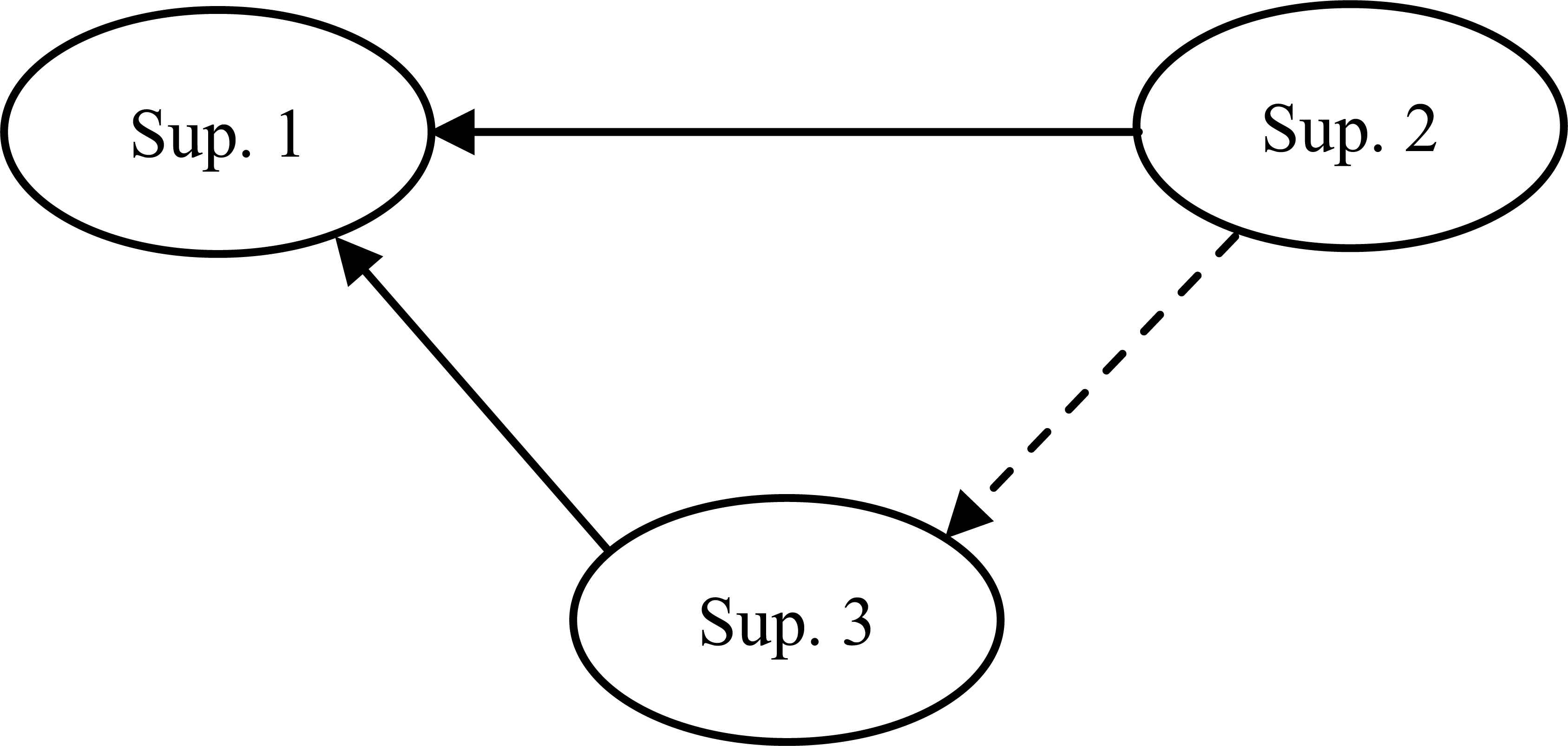
Fuzzy Kernel graph

5. Conclusion

In this study, ELECTRE I outranking method using hesitant fuzzy linguistic term set is proposed. Since decision making involves uncertainty and imprecision, DMs prefer to render linguistic judgments about decision alternatives and criteria. Our proposed method facilitates decision making process due to using comparative linguistic expressions to evaluate the alternatives and criteria and it could be a DM-friendly MCDA method. Fuzzy sets theory and subsequent developments empowers us to numerically interpret the uncertainty of MCDA problems. Ultimately, ELECTRE I method is established to investigate binary relations of alternatives and criteria in order to compare them by comparative linguistic terms.

In this proposed HFLTS-ELECTRE I method, the combination matrix of concordance and discordance remains fuzzy. Our method offers an evolution in outranking relations through elimination of concordance and discordance thresholds form ELECTRE I method. Hence, we propose fuzzy Kernel diagram to represent the preferences of actions. This new diagram uses dashed lines to depict decision maker’s uncertainty toward actions. Since fuzzy Kernel diagram is implemented, defuzzification of the fuzzy concordance matrix is not needed and we continue the calculations by fuzzy values until the final step. Thus, the output clearly illustrates decision maker’s assessments and his/her preferences. Future works could focus on extensions of HFLTS for other members of ELECTRE family or outranking methods. In addition, extension of fuzzy Kernel diagram could represent decision maker’s preferences in detail.