
An approach for solving maximal covering location problems with fuzzy constraints
- DOI
- 10.1080/18756891.2016.1204121How to use a DOI?
- Keywords
- Location Problems; Maximal Covering; Uncertainty; Soft Computing; Fuzzy sets
- Abstract
Several real-world situations can be modeled as maximal covering location problem (MCLP), which is focused on finding the best locations for a certain number of facilities that maximizes the coverage of demand nodes located within a given exact coverage distance (or travel time). In a real scenario, such distance as well as other elements of the location problem can be uncertain or linguistically (vaguely) defined by the decision maker. In this paper, we manage flexibility in the coverage distance through a fuzzy constraint. So, an extension of the original MCLP model is proposed, which is solved by using a parametric approach. Computational experiments have been conducted to analyze how the proposed model can be solved and what kind of information can be obtained to help a potential decision maker to take a more informed decision.
- Copyright
- © 2016. the authors. Co-published by Atlantis Press and Taylor & Francis
- Open Access
- This is an open access article under the CC BY-NC license (http://creativecommons.org/licences/by-nc/4.0/).
1. Introduction
The maximal covering location problem (MCLP) is one of the most used covering problems in the context of the location theory. The MCLP was originally proposed by Church and ReVelle 3 and later reconsidered in 13. Several applications of the MCLP were recently reviewed in 7.
In this problem, a set of demand nodes and a set of facilities to be located are considered. These facilities can be located within the same demand nodes. Each demand node has an associated value, which represent its level of importance (demand generated at the node). The objective of the MCLP is to find the best locations for a fixed number of facilities in order to maximize the demand coverage. As the demand generated at the nodes is taken into account, the nodes with greater demand will be always covered, while some nodes can remain uncovered.
A demand node is considered covered if exist one facility, which can provide the required service at a distance or travel time less than or equal to predefined threshold.
In a recent review we made 8, we observed that, in general, covering location problems are addressed considering that all the parameters of the problem under study are known with certainty. However, in many real situations, uncertainty can be present in some of these parameters, like the demand generated at nodes; the distance between the facilities and the demand nodes; the coverage radius; the server capacity; the installation cost; the aspiration levels; the risks; the arrival rate of demand; etc. Moreno et al. 12 claimed that the vagueness in the location problems could be adequately modeled by networks with fuzzy values which describe nodes, lengths of paths, etc.
Fuzzy approaches have been considered to address uncertainty in the maximal covering location problem 8. Among the parameters with potential uncertain values, we will focus here in the coverage distance which is usually considered exactly known. As a consequence, a demand node is covered if there exist a facility within such coverage distance, while nodes that are beyond this distance are not covered. Thus, for example, nodes that are within a distance of 3.0 kilometers from a facility are fully covered, while those nodes that are at a distance of 3.01 kilometers are not covered. It is clear that this rigidity of the distance could lead to inappropriate and unrealistic solutions for the problem under study and it would be more reasonable to consider that a node is covered if there exist a facility at “approximately 3.0 kms”.
Along this line of research, Davari et al. 4 proposed a model based on a fuzzy approach in which possibility and necessity measures are used for calculating the travel time between the demand nodes and the facilities, and to estimate the expected coverage of demand. Also in 5, the same authors presented a large scale MCLP with fuzzy coverage radius, which is represented by a triangular fuzzy number. Batanović et al. 1 presented a MCLP applied in networks where the demand values are described by linguistic terms and represented by triangular fuzzy numbers. Takaĉi et al. 15 posed a fuzzy maximal covering location model in which the coverage radius is considered as a fuzzy number and defined a coverage degree for the demand nodes. Shavandi and Mahlooji 14 applied a fuzzy approach based on the queuing theory where the demand of the nodes, server capacity, average number of customers at the queue, and service times of servers are considered as triangular fuzzy numbers.
For an in-depth review, considering fuzzy approaches for location problems, models and solving methods, the interested reader can refer to Guzmán et al. 8.
So, given the importance of the MCLP and being clear that the covering distance is a matter of degree, the aim of this paper is to propose a fuzzy extension of the problem that uses a fuzzy constraint to model the standard distance as an uncertain value. In this situation, the decision maker allows some violations in the accomplishment of the distance constraint and, in order to solve the problem, we apply the parametric approach proposed by Verdegay 17, which converts the fuzzy problem into a set of crisp problems. This approach has been successfully used in other relevant applications (e.g. 16,10).
These crisp problems can be solved using well known conventional techniques. In this sense, heuristic and metaheuristic methods have been used in recent years to solve different types of location problems 13,11,5. Here, using a specific metaheuristic we will show how the problem can be solved, and the kind of information we can obtain when using this parametric approach, which in turn, will allow the decision maker to take a more informed decision.
Consequently, this paper is organized as follows. Section 2 presents a formal definition of MCLP and also our fuzzy extension is described. Section 3 shows computational experiments that were realized to validate the fuzzy model prosed. The results obtained and a discussion of the findings is presented in Section 4. Finally, our conclusions are outlined in Section 5.
2. Problem definition and proposed fuzzy approach
In this section, our fuzzy extension is described. But first, the MCLP formulation is presented.
- i,I
- index and set of the demand nodes.
- j,J
- index and set of potential locations for the facilities.
- Ni
- {j ∈ J|di j ≤ S} the set of potential facility locations that can cover the node i within the time or distance S, di j is the distance between the node i and the potential location for the facility j.
- p
- the number of facilities to be located.
- S
- the maximum allowed time or distance to respond to a request.
- wi
- value that represent the demand associated to node i.
- xj
- 1 if a facility is located at the node j, 0 otherwise.
- yi
- represent the coverage of node i, 1 if node is covered (∃j|xj = 1 ∧ j ∈ Ni), 0 otherwise.
Mathematical model
The objective function (1) maximizes the demand covered by the set of established facilities. Constraint (2) states that one or more facilities will be located within the distance or travel time pre-defined S from the demand node i. Constraint (3) ensures that the number of facilities to be located is p. Finally, decision variables xi and yi are considered as binaries.
With the aim to illustrate the above model, Figure 1 shows a feasible solution for a MCLP with two facilities, which cover twenty five demand nodes. The size of the node indicates its demand. Here, two demand nodes are covered by the two facilities and there are uncovered nodes.
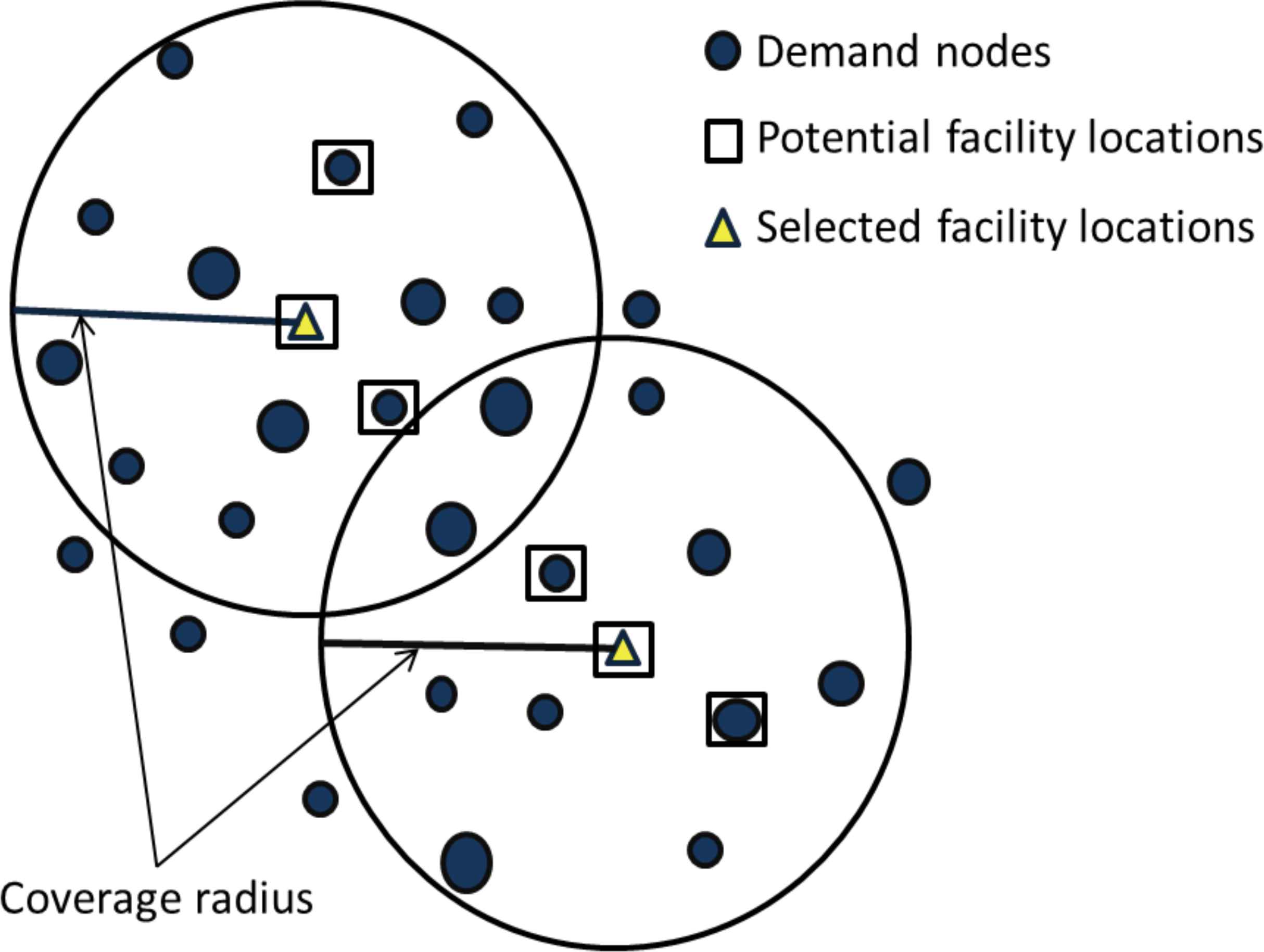
A feasible solution of the MCLP with two facilities, six potential facility locations, and twenty five demand nodes.
As we noted before, because of in real MCLP some elements could be imprecise or vaguely defined, the application of fuzzy sets and systems techniques to model and/or manage such imprecision is fully justified.
In the MCLP, a demand node is covered by a facility if the distance between both is less than a given standard o coverage distance. A decision maker may allow some flexibility on this fact, that, in mathematical terms can be modeled using a fuzzy constraint.
We consider the following fuzzy constraint in the construction of the Ni set:
There are several approaches to transform fuzzy models into classical ones, i.e. crisp models, see, for example, 2,6,18. As mentioned in the introduction, the parametric approach proposed by Verdegay 17 is used to solve our fuzzy extension of the MCLP. Basically, this approach employs two phases, the first one transforms the fuzzy problem into several crisp problems by using α-cuts, where the parameter α ∈ [0,1] represents the satisfaction degree of the decision maker. As a consequence, for each α ∈ [0,1] considered, a classical MCLP (α-MCLP) is obtained. In the second phase, all these problems are solved by classical optimization techniques. The results obtained for the different α values generate a set of solutions, which could be integrated by the Representation Theorem for fuzzy sets. Thus, we can say that the solution provided by the parametric approach is a solution of our fuzzy MCLP extension. See Figure 2.
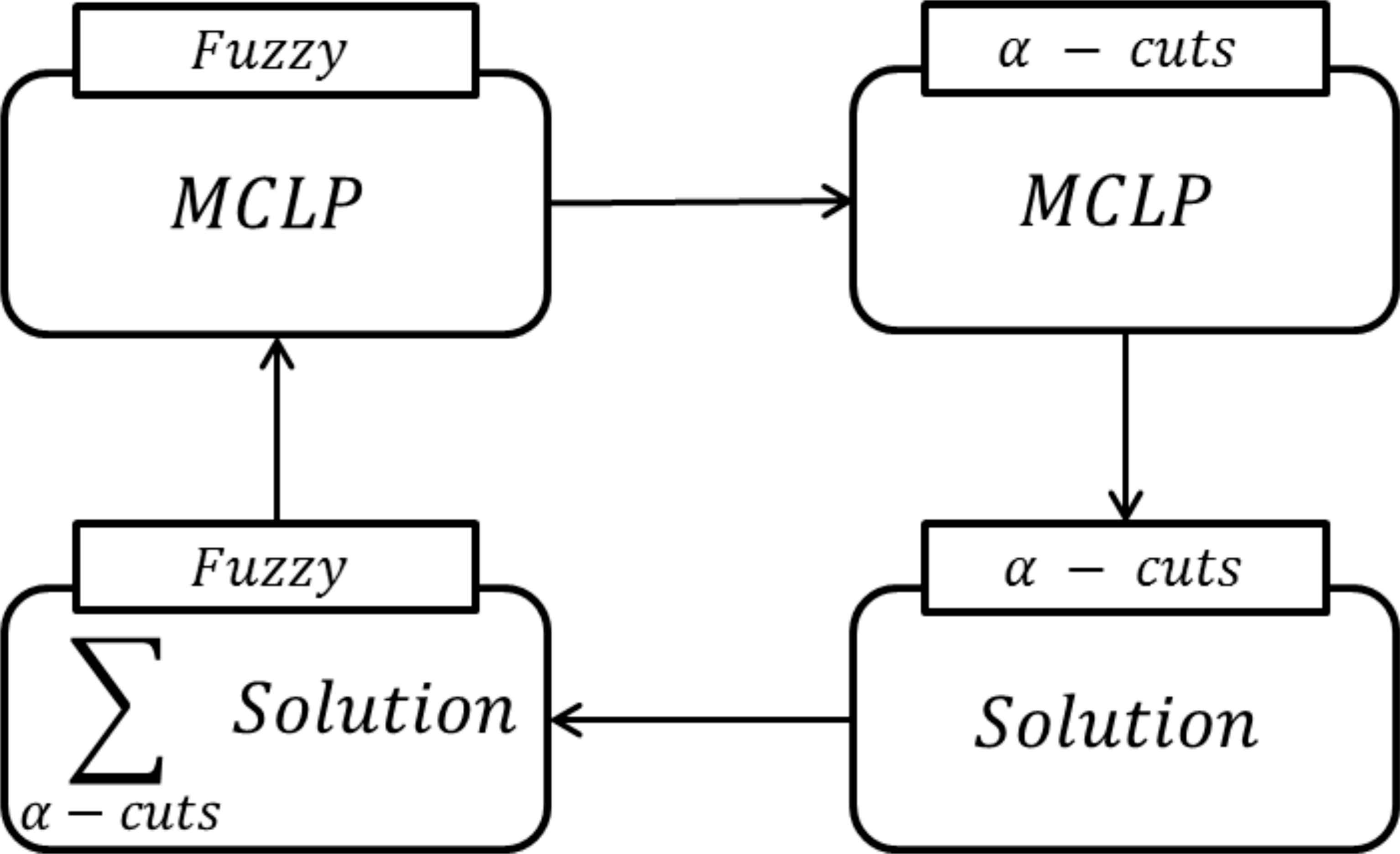
Parametric approach applied to the fuzzy MCLP.
Following this approach, Eq. (6) is transformed into the following constraint:
3. Computational experiments
In this Section, computational experiments that were carried out on various scenarios are presented. The proposed model is validated and the solution method is tested.
Test Problem
We follow the guidelines presented in ReVelle et al. 13 to construct the test problem.
The demand nodes were randomly located in a 30 × 30 grid following a uniform distribution. Each node’s demand is uniformly selected at random from the interval [1,50].
Given this scenario, we consider the number of facilities p to be located in the range [1,2,…,11]. The coverage distance is set to S = 5.
All demand nodes are potential locations to establish the facilities and it is assumed that the installation cost is the same for all facilities, so that this cost is not considered in the model. Furthermore, all facilities to be located are homogeneous, that is, it assumed that they have the same response capacity. The Euclidean distance was used to calculate the distance between facilities and demand nodes.
The level of tolerance τ in the distance constraint (8) is set to τ = 1.5 (meaning a maximum of 30% excess from the value of S, when α = 0).
Now, for every value of p we consider different values for the α-cuts. In our experiments we define α ∈ [1.0,0.9,…,0.0], thus leading to a set of 11 crisp problems that need to be solved.
The solving method is described in the next subsection.
Iterated Local Search algorithm
The Iterated Local Search algorithm (ILS) posed in 9 was used to solve our proposed model. This method consists starts with an initial solution s0; and a conditional loop with two main steps: (i) perturbation applied to s0 to obtain a new solution s1; and (ii) local search method used to transform s1 into a local optimum s2. The ILS pseudo-code is shown in Algorithm 1. The perturbation mechanism favors the exploration of other regions of the search space, allowing to escape from local optima, whereas the local search performs the intensification, which allows us to find the best solution within a neighborhood.
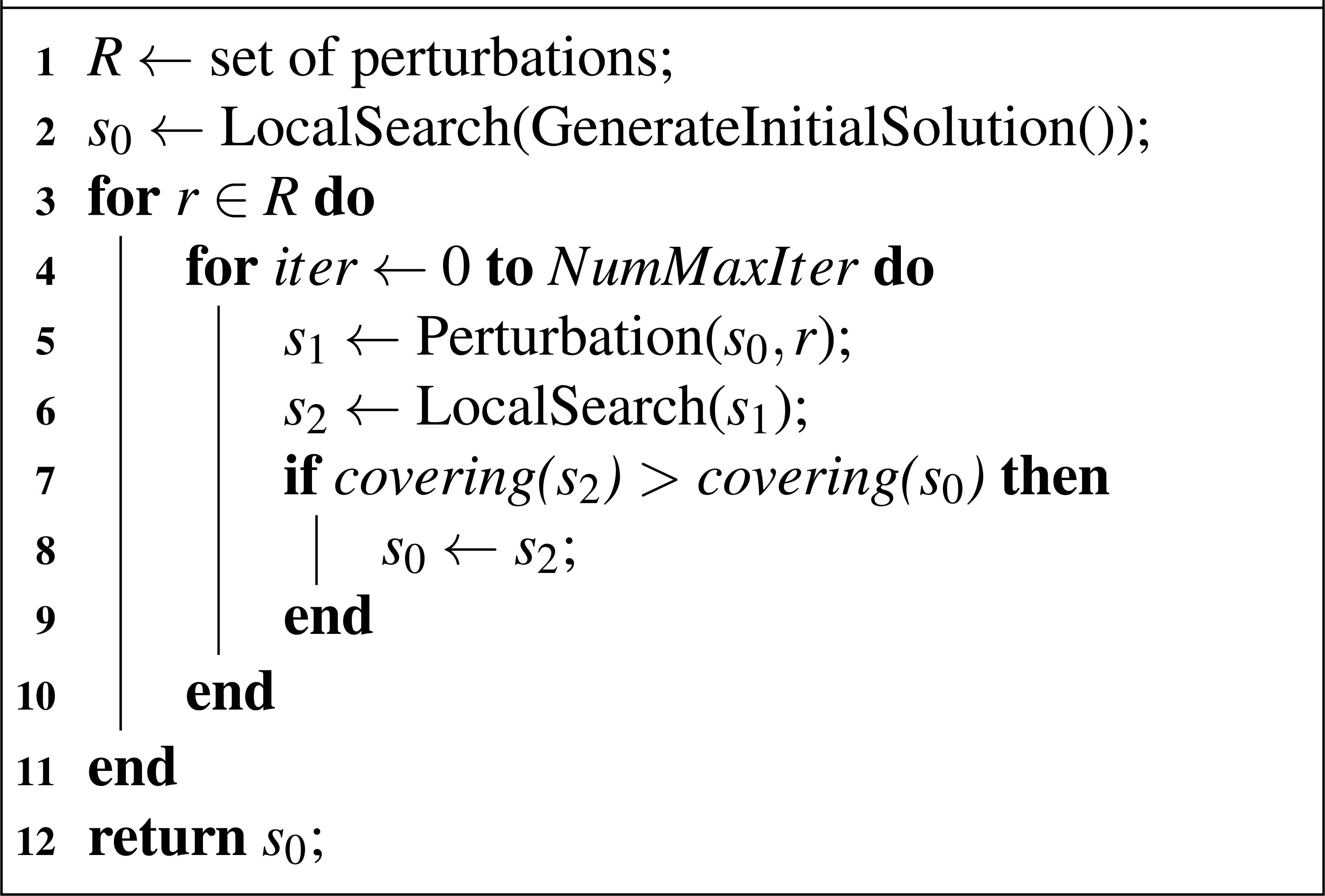
Pseudo-code for the Iterated Local Search method.
Representation of solutions
A solution is simply a vector of size p indicating the node where each one of the p facilities is located. For example, considering 100 demand nodes and 5 facilities, a feasible solution can be represented by the vector s = [10,25,45,80,90], where the first facility will be located in the demand node 10, the second facility will be located in the demand node 25, and so on.
Now, in order to generate an initial solution, we simply assign every facility to a random location without repetition.
Local search procedure
The main idea of local search method is to improve the value of the objective function through a set of movements performed in the solution space. The basic move consist in re-allocating a selected facility.
Once a facility j is selected, the possible new locations are those that are at a distance closer than S (recall that this is a problem’s parameter).
The new location will be the one that maximizes the improvement of the objective function.
In our case, since a facility can be distributed on the set J of potential locations, in this step, for each location j ∈ J, we explore its neighborhood and we replaced it by its best improving neighbor j′. That is to say, that neighbor which maximizes the demand coverage.
- 1.
Randomly select one facility ( j) from the current solution s.
- 2.
For j, obtain its neighbor locations, N = {n | distance(j,n) ≤ S}.
- 3.
For each n ∈ N :
- (a)
s′ := s
- (b)
move facility j to location n in s′
- (c)
if coverage(s′) > coverage(s) then bestN = n
- (a)
- 4.
move facility j to location bestN in s
This process is repeated for a certain number of times that gives the so called depth of the local search.
Perturbation procedure
The perturbation mechanism applies the same basic move as the local search but depending on a different radius that is defined as r here. This parameter r changes during the run of the ILS procedure and we consider the following values r = {5.5,7,8.5,10}. As the radius increases, the set of potential new locations for a given facility also increases, thus allowing to move it far away from the current location. The selected values correspond to percentages of increase of {10%,40%,70%,100%} with respect to the distance S.
Given a solution s and a neighborhood radius r, the pseudo-code for the perturbation procedure is as follows:
- 1.
Choose randomly one facility j of the current solution s.
- 2.
For j, obtain its neighbor locations, N = {n | distance(j,n) ≤ r}.
- 3.
Choose randomly one location n ∈ N and move j to n.
Computational Experiments
Both the model and the algorithm ILS were programmed using Java and compiled with Eclipse 4.2.2.
For each α ∈ {1.0,0.9,…,0.0} and for each p ∈ {1,2,3,…,11}, we perform 30 independent runs of the ILS method, thus having a total of 11 × 11 × 30 = 3630 runs.
Every run uses 400 iterations. Every 100 iterations, the value of r is changed. At the end, every run makes 400 × 10000 evaluations of the objective function. The best (maximum) solution found in each run was recorded.
The experiments were conducted on a notebook with an Intel Core i5 at 2.4 GHz running Windows 7 64-bit operating system and with 8 GB of RAM.
4. Results and discussion
The results can be analyzed from several points of view.
We start with Table 1, where for each value of α and number of facility (p) the maximum coverage percentage (over 30 runs) is shown.
| α-cut | Number of facilities | ||||||||||
|---|---|---|---|---|---|---|---|---|---|---|---|
| 1 | 2 | 3 | 4 | 5 | 6 | 7 | 8 | 9 | 10 | 11 | |
| 1.0 | 14.40 | 27.58 | 37.50 | 47.44 | 56.23 | 63.88 | 71.56 | 78.98 | 82.93 | 88.04 | 92.86 |
| 0.9 | 14.96 | 28.59 | 40.86 | 50.06 | 60.16 | 66.53 | 75.16 | 80.72 | 88.31 | 91.50 | 93.13 |
| 0.8 | 14.96 | 28.59 | 40.86 | 49.77 | 58.11 | 66.72 | 73.87 | 81.49 | 89.20 | 93.38 | 93.77 |
| 0.7 | 15.18 | 30.29 | 42.57 | 53.25 | 61.34 | 68.76 | 77.93 | 85.48 | 89.24 | 93.09 | 96.09 |
| 0.6 | 15.18 | 30.29 | 42.57 | 53.25 | 60.18 | 70.09 | 77.89 | 84.38 | 90.32 | 92.08 | 95.16 |
| 0.5 | 15.99 | 31.17 | 43.59 | 53.33 | 63.32 | 70.87 | 80.20 | 86.22 | 91.50 | 95.24 | 97.46 |
| 0.4 | 18.08 | 34.63 | 48.24 | 59.62 | 68.97 | 76.19 | 84.71 | 90.19 | 92.12 | 95.93 | 96.44 |
| 0.3 | 19.03 | 35.58 | 49.19 | 60.57 | 69.38 | 76.58 | 84.61 | 88.35 | 93.79 | 95.78 | 96.17 |
| 0.2 | 19.94 | 38.06 | 52.38 | 63.16 | 71.72 | 79.40 | 85.52 | 92.01 | 94.99 | 97.19 | 96.73 |
| 0.1 | 20.48 | 38.62 | 53.93 | 65.27 | 75.75 | 82.15 | 88.95 | 94.72 | 97.89 | 98.51 | 99.42 |
| 0.0 | 21.33 | 40.38 | 56.66 | 69.14 | 79.64 | 85.52 | 91.44 | 97.95 | 98.61 | 99.46 | 99.69 |
| Difference | 6.9 | 12.8 | 19.2 | 21.7 | 23.4 | 21.6 | 19.9 | 19.0 | 15.7 | 11.4 | 6.8 |
| Average coverage | 17.2 | 33.1 | 46.2 | 56.8 | 65.9 | 73.3 | 81.1 | 87.3 | 91.7 | 94.6 | 96.1 |
Coverage percentages obtained for different α-cuts and different numbers of facilities.
The last two rows have a special meaning. The ”Difference” row, shows the coverage difference obtained between α = 0.0 and α = 1.0 (the less restrictive and the more restrictive versions of the constraint, respectively). The “Average coverage” is simply the average of the coverage for all the values of α.
The data shown in Table 1 provide a range of solutions that allows to explore the results from different perspectives by observing variations in the rates of coverage generated by changes in the number of facilities, in the α-level or both values. When reading the table by columns, we observe that as α decreases (the constraint relaxation increases), the coverage percentage also increases. Looking at any specific α-cut, is it clear that coverage can be increased adding more facilities.
Regarding the “Difference” row, the values are positive, meaning that the percentages of coverage with α = 0.0 are always greater than those of α = 1.0. In some cases, the relaxation of the constraint satisfaction led to an improvement that ranges from approx. 7% with 1 or 11 facilities, to up more than 20% when using 4, 5 or 6 facilities. As we will comment later, this is not exclusively due to the fact that as the coverage distance increases, more nodes are covered.
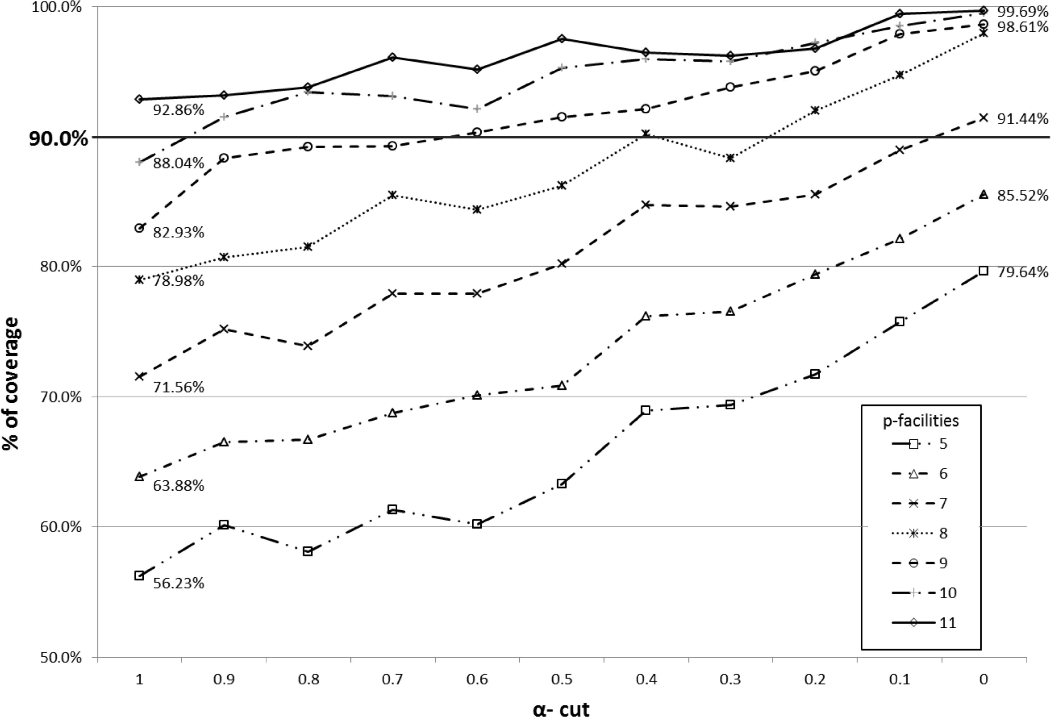
If we focus on a specific percentage of coverage, we note that this value can be obtained in different ways. For example, the results shown in bold represent a percentage of coverage greater than or equal to 90%. Figure 3 shows a graph of the coverage percentage obtained for the different number of facilities 5 to 11, and for all the α-cuts. The x axis indicates the values of α, whereas the y axis indicates the coverage percentages. The curves represent the evolution of the coverage percentage obtained for each number of facilities. In most cases, a decrease in α increases the coverage percentage except for some particular cases where this percentage is the same or decreases. Such decrease in the percentage probably is caused by the method of resolution that we have applied.
Coverage percentage attained for each number of facilities considered and α-cut.
This kind of plot is very useful for a decision maker. For example, if he wants a coverage percentage around 90%, he can draw a line as the one shown in the plot and check which series intersect. It can be observed that such level of coverage can be achieved using from 7 to 11 facilities, of course using certain flexibility in the standard distance (different α value). Having this in mind, the decision maker can decide to increase the number of facilities or to be more tolerant with respect to the distance. This is of utmost importance if, for example, the installation cost of the facilities are later taken into account.
As mentioned before, increasing the number of facilities increases the percentage of coverage. However, the contribution to the global coverage associated to a new added facility decreases. That is, the percentage of coverage given by facility p is less than the percentage of coverage obtained by the facility p − 1. Table 2 shows the percentage of coverage attained for each added facility. For some specific values of α, this percentage is less than 1% (see bold values for facilities 9, 10, and 11).
| α-cut | Number of facilities | ||||||||||
|---|---|---|---|---|---|---|---|---|---|---|---|
| 1 | 2 | 3 | 4 | 5 | 6 | 7 | 8 | 9 | 10 | 11 | |
| 1.0 | 14.40 | 13.18 | 9.91 | 9.95 | 8.79 | 7.65 | 7.68 | 7.41 | 3.95 | 5.11 | 4.82 |
| 0.9 | 14.96 | 13.63 | 12.27 | 9.19 | 10.10 | 6.37 | 8.63 | 5.56 | 7.59 | 3.19 | 1.63 |
| 0.8 | 14.96 | 13.63 | 12.27 | 8.90 | 8.34 | 8.61 | 7.14 | 7.63 | 7.70 | 4.18 | 0.39 |
| 0.7 | 15.18 | 15.12 | 12.27 | 10.69 | 8.09 | 7.41 | 9.18 | 7.55 | 3.76 | 3.85 | 3.00 |
| 0.6 | 15.18 | 15.12 | 12.27 | 10.69 | 6.93 | 9.91 | 7.80 | 6.48 | 5.94 | 1.76 | 3.08 |
| 0.5 | 15.99 | 15.18 | 12.43 | 9.74 | 9.99 | 7.55 | 9.33 | 6.02 | 5.28 | 3.74 | 2.23 |
| 0.4 | 18.08 | 16.55 | 13.61 | 11.38 | 9.35 | 7.22 | 8.52 | 5.48 | 1.94 | 3.81 | 0.50 |
| 0.3 | 19.03 | 16.55 | 13.61 | 11.38 | 8.81 | 7.20 | 8.03 | 3.74 | 5.44 | 1.99 | 0.39 |
| 0.2 | 19.94 | 18.12 | 14.32 | 10.78 | 8.56 | 7.68 | 6.12 | 6.48 | 2.98 | 2.21 | 0.46 |
| 0.1 | 20.48 | 18.14 | 15.31 | 11.34 | 10.47 | 6.41 | 6.79 | 5.77 | 3.17 | 0.62 | 0.91 |
| 0.0 | 21.33 | 19.05 | 16.28 | 12.49 | 10.49 | 5.88 | 5.92 | 6.50 | 0.66 | 0.85 | 0.23 |
Individual contribution to the percentage of coverage by each added facility, for different α-cuts.
Figure 4 shows the average percentage of coverage given for each facility. The highest coverage is given by the first facilities, and that there is a decreasing tendency as more facilities are added. This tendency is clearly linear (R2 = 0.9726). The reader can observe a slight perturbation at the seventh facility, however this is a consequence of using an approximate resolution method and has no other additional impact.
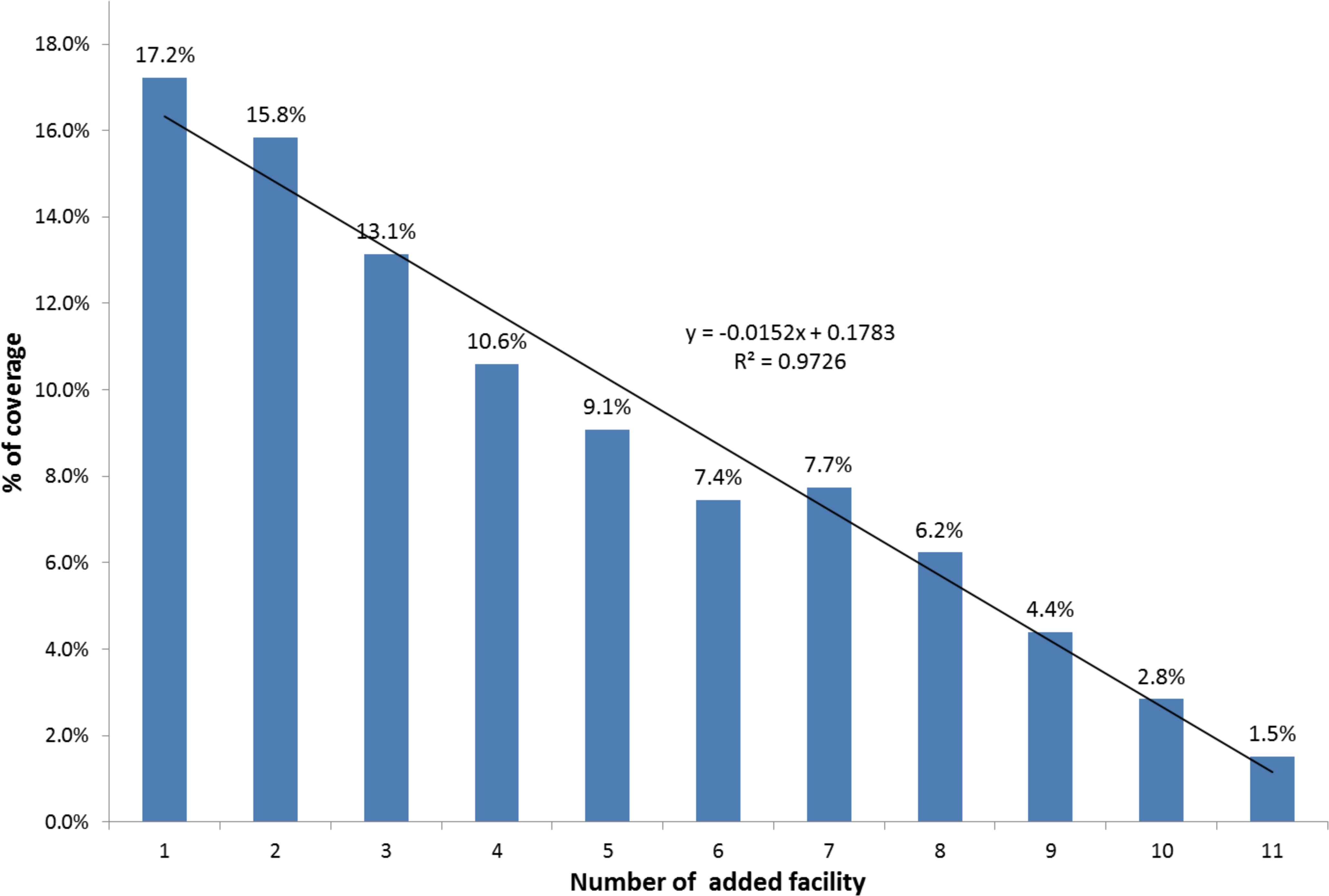
Average percentage of coverage (over different values of α) achieved by each added facility.
Finally, we analyze the impact that the constraint relaxation has on the distribution of facilities. Figure 5 shows a group of 6 graphs representing solutions of three different scenarios of the MCLP extension proposed in this research. Each row corresponds to solutions with 6, 8, and 10 facilities (from top to bottom) and α = 1.0 (left) and α = 0.0 (right). In every case, the solution and the coverage percentage obtained is shown.
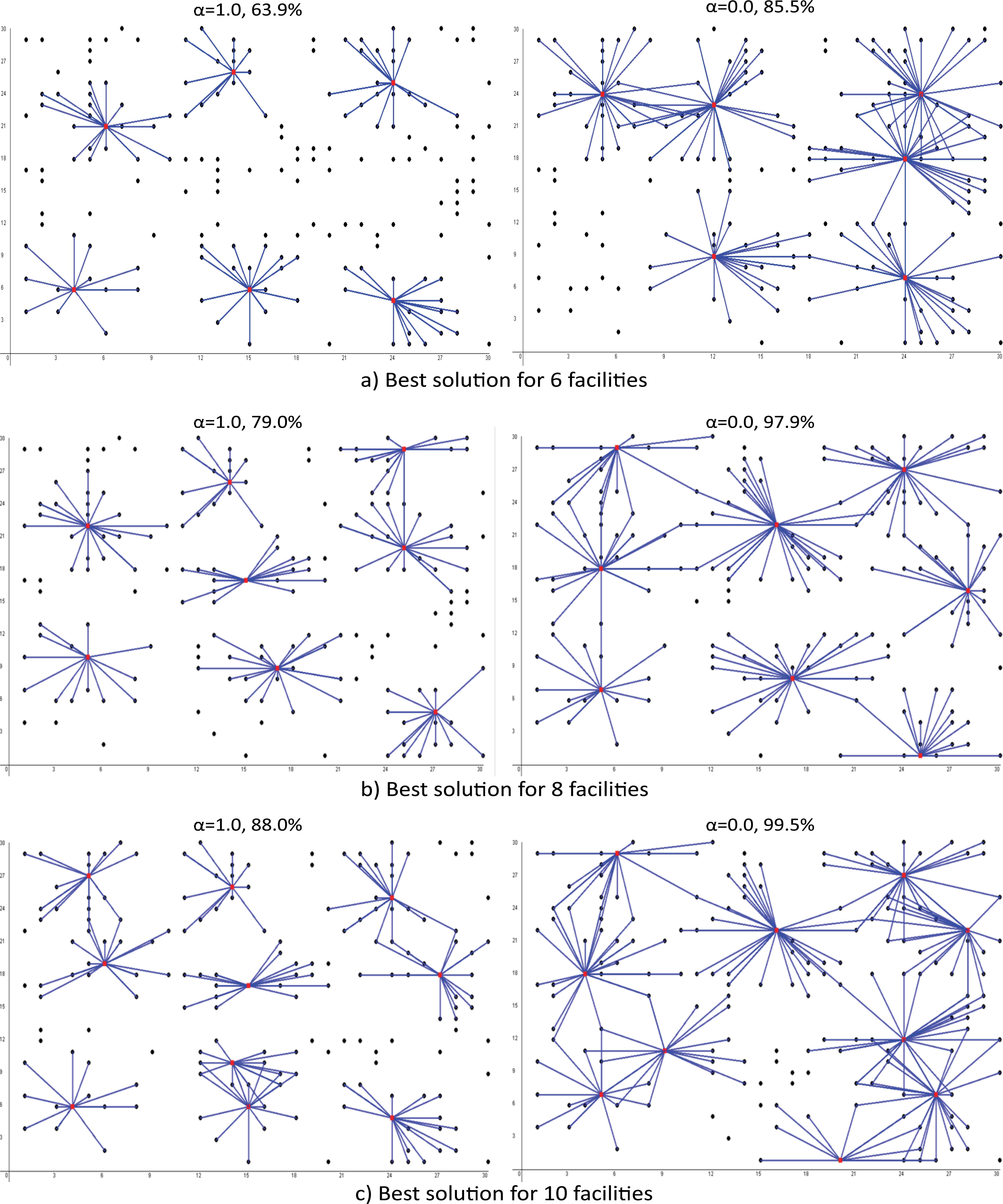
Solutions with different number of facilities (6, 8, and 10) and values of α = 1.0 and α = 0.0.
Due to the relaxation of the distance constraint when α = 0.0, we can see that the amount of covered nodes is always greater than when α = 1.0, thus generating a higher percentage of coverage. It should be also noted that, this increase in coverage is due not only to the fact of relaxing the distance, but also is caused by changes in the facilities locations. That is, these locations change according to the distance value. This means that a location can be the best at a given specific distance value but not the best in others cases.
On the other hand, we can note that in most cases when α = 0.0 there is a significant number of nodes that are covered by more than one facility. This side (and non planned) effect is appropriate in practical applications where it is important to locate backup facilities that respond to customers when the main facilities are not available.
5. Conclusions
In this work, we proposed an extension of the maximal covering location problem using a fuzzy constraint on the distance. In order to solve the resulting model, we focused in a parametric approach, that led to a set of “crisp” problems that, in turn, were solved using an iterated local search heuristic.
Using a randomly generated scenario, we made a set of computational experiments considering different tolerances and number of facilities.
The results obtained allowed to show which kind of information can be gained when using the proposed model. In particular, two aspects should be highlighted: a) availability of information regarding different ways to attain a given percentage of desired coverage; b) opportunity to visually analyze the solutions for different levels of constraint relaxation, which in turn allows to detect the more critical facilities locations (for example, those that are fixed in all the solutions).
Overall, we can conclude that the use of the proposed model coupled with the solving method described, can lead a decision maker to take more informed decisions.
Acknowledgements
This work has been supported by the research projects TIN2014-55024-P and P11-TIC-8001 from the Spanish Ministry of Economy and Competitiveness, and Consejería de Economía, Innovación y Ciencia, Junta de Andalucía (both include European Regional Funds) respectively.
V. C. Guzmán is supported by a scolarship from PROMEP, México, PROMEP/103.5/12/6059.
References
Cite this article
TY  - JOUR
AU  - Virgilio C. Guzmán
AU  - David A. Pelta
AU  - José L. Verdegay
PY  - 2016
DA  - 2016/08/01
TI  - An approach for solving maximal covering location problems with fuzzy constraints
JO  - International Journal of Computational Intelligence Systems
SP  - 734
EP  - 744
VL  - 9
IS  - 4
SN  - 1875-6883
UR  - https://doi.org/10.1080/18756891.2016.1204121
DO  - 10.1080/18756891.2016.1204121
ID  - Guzmán2016
ER  -