
A Novel ACO-Based Static Task Scheduling Approach for Multiprocessor Environments
- DOI
- 10.1080/18756891.2016.1237181How to use a DOI?
- Keywords
- Ant colony optimization (ACO); metaheuristics; multiprocessor task scheduling; parallel and distributed systems
- Abstract
Optimized task scheduling is one of the most important challenges in parallel and distributed systems. In such architectures during compile step, each program is decomposed into the smaller segments so-called tasks. Tasks of a program may be dependent; some tasks may need data generated by the others to start. To formulate the problem, precedence constraints, required execution times of tasks, and communication costs among them are modeled using a directed acyclic graph (DAG) named task-graph. The tasks must be assigned to a predefined number of processors in such a way that the program completion time is minimized, and the precedence constraints are preserved. It is well known to be NP-hard in general form and most restricted cases; therefore, a number of heuristic and meta-heuristic approaches have so far been proposed in the literature to find near-optimum solutions for this problem. We believe that ant colony optimization (ACO) is one of the best methods to cope with such kind of problems presented by graph. ACO is a metaheuristic approach inspired from social behavior of real ants. It is a multi-agent approach in which artificial ants (agents) try to find the shortest path to solve the given problem using an indirect local communication called stigmergy. Stigmergy lets ACO to be fast and efficient in comparison with other metaheuristics and evolutionary algorithms. In this paper, artificial ants, in a cooperative manner, try to solve static task scheduling problem in homogeneous multiprocessor environments. Set of different experiments on various task-graphs has been conducted, and the results reveal that the proposed approach outperforms the conventional methods from the performance point of view.
- Copyright
- © 2016. the authors. Co-published by Atlantis Press and Taylor & Francis
- Open Access
- This is an open access article under the CC BY-NC license (http://creativecommons.org/licences/by-nc/4.0/).
1. Introduction
Today, the utilization of multiprocessor systems has been increased due to increase in time complexity of the programs and decrease in hardware costs. In such systems, programs are divided into the smaller and dependent segments named tasks. Some tasks need the data generated by the other tasks; hence, the problem can be modeled using a directed acyclic graph (DAG) so-called task graph. In the task graph, nodes are tasks and edges indicate the precedence constraints between tasks. The required execution time of each task, communication costs, and precedence constraints are specified during the program’s compile step. Tasks should be mapped into the processors with respect to their precedence so that the overall finish time of the given program is minimized.
Multiprocessor task scheduling problem is NP-hard [1], and achieving the best possible solution is generally too time-consuming and maybe impossible specially for entries with high dimensions; therefore, we have to use intelligent approaches to find near-optimum solutions. Different algorithms proposed to schedule multiprocessor task graph [2], [3] are divided into the two categories: heuristics and non-heuristics. Some of the heuristics named TDB (Task Duplication Based) such as PY1 [4], DSH2 [5], LWB3 [6], BTDH4 [7], LCTD5 [8], CPFD6 [9], MJD7 [10], and DFRN8 [11] allow task duplication over processors to skip over the communication costs between tasks and their children in order to make the finish time shorter. There are two important issues to be addressed for designing an effective task duplication technique. 1) Which nodes to duplicate? 2) Where to duplicate the nodes? Furthermore, task duplication requires more memory, and cannot be used for some applications such as bank-transactions.
Other heuristics do not allow task-duplication, themselves are divided into the two groups. First, the UNC (Unbounded Number of Clusters) methods such as LC9 [12], EZ10 [13], MD11 [14], DSC12 [15], and DSP13 [16], which assume an unbounded number of processors using task-graph clustering. That is, they part the given task-graph into the some clusters, and then assign the clusters to the processors. They find the optimal number of processors implicitly. However, unlimited number of processor elements (or a large number of ones) may not be available in the real problems. Actually, in most the cases, the number of processors is predefined and constant.
Second, the BNP (Bounded Number of Processors) methods such as HLFET14 [17], ISH15 [5], CLANS16 [18], LAST17 [19], EFT18 [20], DLS19 [21], and MCP20 [14], in which the number of processors are restricted using list-scheduling technique (the proposed approach is in this group). They make a list of ready-tasks at each stage, and assign them some priorities. Then, the most priority task in the ready-list is selected to schedule on the processor that allows the earliest start time, until all the tasks are scheduled.
Finally, among non-heuristic approaches, one can see genetic algorithm (GA) [22]–[32], simulated annealing (SA) [33], and local search [34]. Although genetic algorithm has a significant contribution, the necessary time for its execution is usually more than random running of the tasks, especially in the given entries with low dimensions; therefore, trends to apply the faster and more efficient methods such ant colony optimization have been raised a lot nowadays.
Ant colony optimization (ACO) is a meta-heuristic approach simulating social behavior of real ants. Ants always find the shortest path from the nest to the food and vice versa. Artificial counterparts try to find the shortest solution of the given problem on the same basis. Dorigo et al. first utilized ant algorithm as a multi-agent approach to solve the traveling sales man problem (TSP) [35] and after that, it has been successfully used to solve a large number of difficult discrete optimization problems [36].
The author was the first who applied ACO to the static multiprocessor task-graph scheduling [46], though the introduced approach had some drawbacks. First of all, the priority measurements were not included in the study, while the utilization of them as heuristic values push the ACO algorithm by far ahead. Second, the experiments were conducted only on the small input task graphs, while in this paper a comprehensive set of large-scale task graphs have been introduced, and the behavior of the proposed approach on them have been carefully studied. We believe the most contribution of this work is to classify and formulate the static task-graph scheduling in homogeneous multiprocessor environments in a clear and comprehensive way, and to propose a novel framework based on the ACO, which is superior in comparison with the traditional procedures.
The organization of the rest of the paper is as follows. In the following Section, multiprocessor task scheduling problem is surveyed in detail. Ant colony optimization is discussed in the Section 3. Section 4 introduces the proposed approach. Section 5 is devoted to implementation details and the results, and finally, the paper is concluded in the last Section.
2. Multiprocessor Task Scheduling
A directed acyclic graph G = {N, E, W, C} named task graph is used to model the multiprocessor task scheduling problem, where N = {n1, n2,…, nn}, E = {(ni, nj) | ni, nj ∈ N} W = {w1, w2,…, wn}, C = {c(ni, nj) |(ni, nj) ∈ E), and n are set of nodes, set of edges, set of weights of nodes, set of weights of edges, and the number of nodes, respectively.
Fig. 1 shows a task graph for a real program consisting of nine tasks. In this graph, nodes are tasks and edges specify precedence constraints between tasks. Edge (ni, nj) ∈ E demonstrates that task ni must be finished before the starting of task nj. In this case, ni is called a parent, and nj is called a child. Nodes without any parents and nodes without any children are called “entry nodes” and “exit nodes”, respectively. Each node weight like wi is the necessary execution time of task ni, and weight of edge like c(ni, nj) is the required time for data transmission from task ni to task nj identified as communication cost. If both ni and nj are executed on the same processor, the communication cost will be zero between them. Tasks execution time and precedence constraints between tasks are generated during the program compiling-stage. Tasks should be mapped into the given m processor elements according to their precedence so that the overall finish time of the tasks would be minimized.
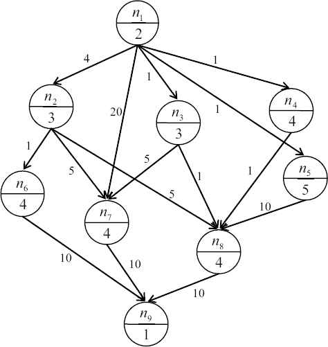
Task graph of a program with nine tasks [32].
Most BNP scheduling algorithms are based on the so-called list-scheduling technique. The basic idea behind list-scheduling is to make a sequence of nodes as a list for scheduling by assigning them some priorities, then repeatedly removing the most priority node from the list, and allocating it to the processor that allows the earliest-start-time (EST), until all the nodes in the graph are scheduled. The results achieved by such BNP methods are dominated by two major factors. Firstly, which order of tasks should be selected (sequence subproblem), and secondly, how the selected order should be assigned to the processors (assigning subproblem).
If all the parents of task ni were executed on the processor pj, EST(ni, pj) would be Avail(pj), that is the earliest time at which pj is available to execute the next task. Otherwise, the earliest-start-time for task ni on processor pj should be computed using
For a given task-graph with n tasks using its adjacency matrix, an efficient implementation for assigning all the tasks in the task-graph to a given m identical processors using EST method has a time-complexity belonging to the O(mn2) [2].
Some frequently used attributes to assign priority to the tasks are TLevel (Top-Level), BLevel (Bottom-Level), SLevel (Static-Level), ALAP (As-Late-As-Possible), and the new proposed NOO (The-Number-Of-Offspring) [47]. The TLevel or ASAP (As-Soon-As-Possible) of a node ni is the length of the longest path from an entry node to the ni excluding ni itself, where the length of a path is the sum of all the nodes and edges weights along the path. The TLevel of each node in the task graph can be computed by traversing the graph in topological order using
The BLevel of a node ni is the length of the longest path from ni to an exit node. It can be computed for each task by traversing the graph in the reversed topological order as follows:
If the edges weights are not considered in the computation of BLevel, a new attribute called Static-Level or simply SLevel can be generated using (5).
The ALAP start-time of a node is a measure of how far the node’s start-time can be delayed without increasing the overall schedule-length. It can be drawn for each node by using (6).
Finally, the NOO of ni is simply the number of all its descendants (or offspring). Table 1 lists the abovementioned measures for each node in the task graph of Fig. 1.
| Node | TLevel | BLevel | SLevel | ALAP | NOO |
|---|---|---|---|---|---|
| n1 | 0 | 37 | 12 | 0 | 8 |
| n2 | 6 | 23 | 8 | 14 | 4 |
| n3 | 3 | 23 | 8 | 14 | 3 |
| n4 | 3 | 20 | 9 | 17 | 2 |
| n5 | 3 | 30 | 10 | 7 | 2 |
| n6 | 10 | 15 | 5 | 22 | 1 |
| n7 | 22 | 15 | 5 | 22 | 1 |
| n8 | 18 | 15 | 5 | 22 | 1 |
| n9 | 36 | 1 | 1 | 36 | 0 |
TLevel, BLevel, SLevel, ALAP, and NOO of each node in the task graph of Fig. 1.
To open up how these measures can be utilized in order to schedule tasks of a task-graph, four well-known traditional list-scheduling algorithms (of course, on behalf of the BNP class) are surveyed as follows.
2.1. The HLFET Algorithm
The HLFET (Highest Level First with Estimated Times) [17] first calculates the SLevel of each node in the given task-graph. Then, make a ready-list in the descending order of SLevel. At each instant, it schedules the first node in the ready-list to the processor that allows the earliest-execution-time (using the non-insertion approach) and then, updates the ready-list by inserting the new nodes ready now to be executed, until all the nodes are scheduled. For this algorithm, the time-complexity of the sequencing subproblem for a task-graph with n tasks is O(n2), where assigning tasks to the m given processor using EST belongs to O(mn2). Fig. 2 (a) shows the scheduling Gantt chart of the graph in Fig. 1 using HLFET algorithm on two processor elements.
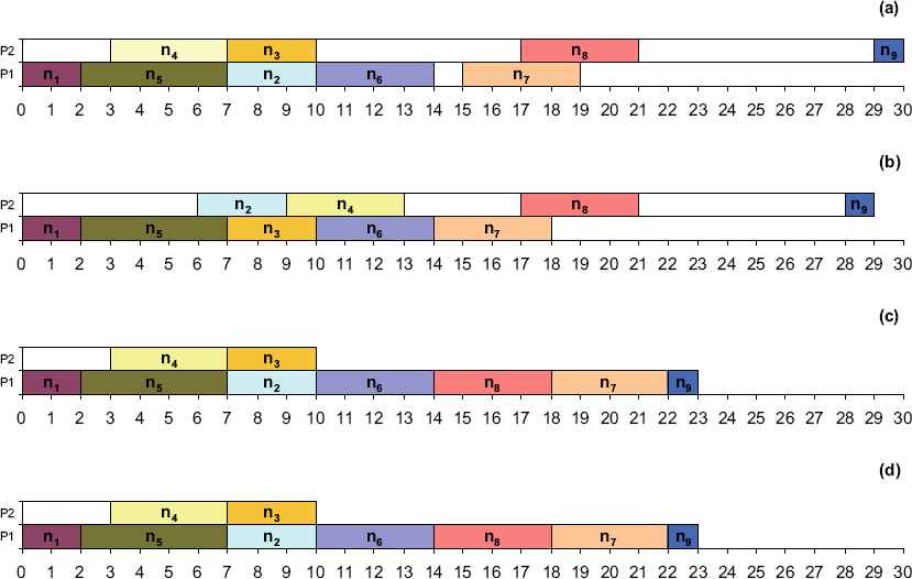
The scheduling of the task graph of Fig. 1 using the four different traditional heuristics. (a) The HLFET algorithm. (b) The MCP algorithm. (c) The DLS algorithm. (d) The ETF algorithm.
2.2. The MCP Algorithm
The MCP (Modified Critical Path) algorithm [14] uses the ALAP of the nodes as priority. It first computes the ALAP times of all the nodes, and then constructs a ready-list in the ascending order of ALAPs. Ties are broken by considering the ALAP times of the children of the nodes. The MCP algorithm then schedules the nodes in the list one by one to the processor that allows the earliest-start-time using the insertion approach. For this algorithm, time-complexity of sequencing subproblem for a task-graph with n tasks is O(n2log n), where assigning tasks to the m given processor using EST belongs to O(mn2). The scheduling of the graph of Fig. 1 using MCP algorithm on two processor elements is shown by Fig. 2 (b).
2.3. The DLS Algorithm
The DLS (Dynamic Level Scheduling) algorithm [21] uses an attribute called dynamic-level (or DL) that is the difference between SLevel of a node and its earliest-start-time on a processor. At each scheduling step, the DLS algorithm computes the DL for every node in the ready-list on all the processors. The node-processor pair that gives the largest DL is selected to schedule, until all the nodes are scheduled. The algorithm tends to schedule nodes in a descending order of SLevel at the beginning, but nodes in an ascending order of their TLevel near the end of the scheduling process. The overall time-complexity of algorithm belongs to O(mn3). Fig. 2 (c) shows scheduling of the graph of Fig. 1 using DLS algorithm on two processor elements.
2.4. The ETF Algorithm
The ETF (Earliest Time First) algorithm [20] computes the earliest-start-times for all the nodes in the ready-list by investigating the start-time of a node on all the processors exhaustively. Then, it selects a node that has the smallest start-time for scheduling; ties are broken by selecting the node with the higher SLevel priority. The overall time-complexity of algorithm belongs to O(mn3). The scheduling of the graph of Fig. 1 using EST algorithm on two processor elements is shown by Fig. 2 (d).
3. Ant Colony Optimization
Ant colony metaheuristic is a concurrent algorithm in which a colony of artificial ants cooperates to find optimized solutions of a given problem. Ant algorithm was first proposed by Dorigo et al. as a multi-agent approach to solve traveling salesman problem (TSP) and since then, it has been successfully applied to a wide range of difficult discrete optimization problems such as quadratic assignment problem (QAP) [37], job shop scheduling (JSP) [38], vehicle routing [39], graph coloring [40], sequential ordering [41], network routing [42], to mention a few.
Leaving the nest, ants have a completely random behavior. As soon as they find a food, while walking from the food to the nest, they deposit on the ground a chemical substance called pheromone, forming in this manner a pheromone trail. Ants smell pheromone. Other ants are attracted by environmental pheromone, and subsequently they will find the food source too. More pheromone is deposited, more ants are attracted, and more ants will find the food. It is a kind of autocatalytic behavior. In this way (by pheromone trails), ants have an indirect communication, which are locally accessible by the ants so-called stigmergy, a powerful tool enabling them to be very fast and efficient. Pheromone is evaporated by sunshine and environmental heat, time by time, destroying undesirable pheromone paths.
If an obstacle, of which one side is longer than the other side, cuts the pheromone trail. At first, ants have random motions to circle round the obstacle. Nevertheless, the pheromone of the longer side is evaporated faster, little by little, ants will convergence to the shorter side, and hereby, they always find the shortest path from food to the nest vice versa.
Ant colony optimization tries to simulate this foraging behavior. In the beginning, each state of the problem takes a numerical variable named pheromone-trail or simply pheromone. Initially these variables have an identical and very small value. Ant colony optimization is an iterative algorithm. In each iteration, one or more ants are generated. In fact, each artificial ant is just a list (called Tabu-list) keeping the visited states by the ant. The generated ant is placed on the start state, and then selects next state using a probabilistic decision based on the value of pheromone trails of the adjacent states. The ant repeats this operation, until it reaches to a final state. In this time, the values of the pheromone variables for the visited states are increased based on the desirability of the achieved solution (depositing pheromone). Finally, all the variables are decreased simulating pheromone evaporation. By mean of this mechanism ants will be converged to the more optimal solutions.
One of the superiorities of ant colony optimization as compared to the Genetic algorithm is, as said before, indirect communication among ants using the pheromone variables. In contrast to the Genetic algorithm, in which decisions are often random and based on the mutation and cross over (many experiences will be also eliminated by throwing the weaker chromosomes away); in ant colony optimization, all decisions are purposeful and based on the cumulative experiments of all the previous ants. This indirect communication enables ant colony optimization to be more preciously and more quickly.
4. The Proposed Approach
At first, an n×n matrix named τ is considered as pheromone variables, where n is the number of tasks in the given task graph. Actually, τij is the desirability of selecting task nj just after task ni. All the elements of the matrix initiate with a same and very small value. Then, the iterative ant colony algorithm is executed. Each iteration has the following steps:
- 1.
Generate ant (or ants).
- 2.
Loop for each ant (until a complete scheduling of all the tasks in the given task-graph).
- -
Select the next task according to the pheromone variables of the ready-tasks using a probabilistic decision-making.
- -
- 3.
Deposit pheromone on the visited states.
- 4.
Daemon activities (to boost the algorithm)
- 5.
Evaporate pheromone.
A flowchart of these operations with more details and a complete implementation in pseudo-code are also shown in Fig. 3 and Fig. 4, respectively. In the first stage, just a list with the length of n, is created as ant. At first, this list is empty, and will be completed during the next stage. In the second stage, there is a loop for each ant. In each iteration, the generated ant must select a task from the ready-list using a probabilistic decision-making based on the values of the pheromone variables and heuristic values (priorities) of the tasks. The desirability of selecting task nj just after selecting task ni at iteration t is obtained by the composition of the local pheromone trail values with the local heuristic values (priorities) as follows:
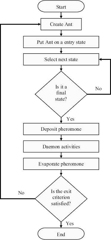
The flowchart of the proposed approach.
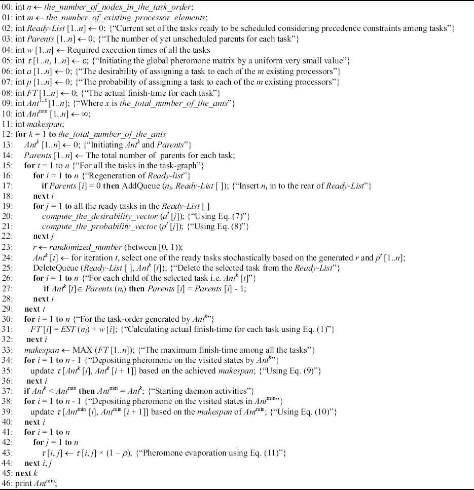
The proposed approach in pseudo-code.
Then a random number is generated, and the next task will be selected according to the generated number; of course, for each ready-task, the bigger pheromone value and the bigger priority, the bigger chance to be selected. The selected task is appended to the ant’s list, removed from the ready-list, and its children ready-to-be-executed-now will be augmented to the ready-list. These operations are repeated, until the complete scheduling of all the tasks, which means the completion of the ant’s list.
In the third stage, tasks are extracted from the ant’s list one by one, and mapped to the processors that supply the earliest-start-time. Then, the maximum finish-time is calculated as makespan that is also the desirability of the obtained scheduling for this ant. According to this desirability, the quantity of pheromone which should be deposited on the visited states is calculated by
In the fourth stage (daemon activity), to intensify and to avoid removing the good solutions, the best-ant-until-now (Antmin), is selected (as the best solution), and some extra pheromone is deposited on the states visited by this ant using
In the last stage, by using (11), pheromone variables are decreased simulating pheromone evaporation in the real environments. It should be taken to avoid premature convergence and stagnation because of the local minima.
5. Implementation Details and Experimental Results
The proposed approach was implemented on a Pentium IV (2.6 GHz LGA) desktop computer with Microsoft Windows XP (SP2) platform using Microsoft Visual Basic 6.0 programming language. All initial values of the pheromone variables were identically set to 0.1. The evaporation rate was considered as 0.998, and the parameters α and β were elected 1 and 0.5 respectively obtained experimentally. The algorithm was terminated after 1500 iterations, that is, after generating 1500 ants.
The implementation of the proposed approach in pseudo-code in Fig. 4 reveals that there are two main iterations in the sequencing subproblem (lines 12, 15, and 16) and (lines 12, 41, and 42) with time-complexity ∈ θ(the_total_number_of_the_ants × n2) where n is the number of tasks in the task graph. Since the_total_number_of_the_ants is a constant initiated to 2500, for the big-enough numbers of n, we can assume that overall time-complexity of the proposed approach in sequencing subproblem belongs to the O(n2), which is equal or better than the traditional preintroduced heuristic methods. On the other hand, the time-complexity of assigning the generated task-order to the existing m processors using EST method (lines 30 and 31) is O(mn2) as usual.
5.1. The Utilized Dataset
Table 2 lists six task graphs of the real-world applications (and their comments) considered to evaluate the proposed approach. These six graphs are the standard ones in the literature, and have utilized to evaluate a number of related works; hence, they let us to compare the proposed approach versus its traditional counterparts. All these six graphs are used to compare the proposed approach against the traditional heuristics, not only the BNP algorithms but also the UNC ones, and then, the proposed approach will be evaluated in comparison with the genetic algorithm using the last two graphs (that are G5 and G6).
| Graph | Comments | Nodes | Communication Costs |
|---|---|---|---|
| G1 | Kwok and Ahmad [2] | 9 | Variable |
| G2 | Al-Mouhamed [43] | 17 | Variable |
| G3 | Wu and Gajski [14] | 18 | 60 and 40 |
| G4 | Al-Maasarani [44] | 16 | Variable |
| G5 | Fig. 1 [32] | 9 | Variable |
| G6 | Hwang et al. [32] | 18 | 120 and 80 |
Selected task graphs for evaluating the proposed approach
In addition, a set of 45 random task graphs are used for better evaluation of the proposed approach. These random task graphs have different shapes on the three following parameters:
- •
Size (n): that is the number of tasks in the task graph. Five different values were considered {32, 64, 128, 256, and 512}.
- •
Communication-to-Computation Ratio (CCR): demonstrate how much a graph is communication or computation base. The weight of each node was randomly selected from uniform distribution with mean equal to the specified average computation cost that was 50 time-instance. The weight of each edge was also randomly selected from a uniform distribution with mean equal to average-computation-cost × CCR. Three different values of CCR were selected {0.1, 1.0, and 5.0}. Selecting 0.1 makes computation intensive task-graphs. In contrast, selecting 5.0 makes communication intensive ones.
- •
Parallelism: the parameter which determine the average number of children for each node in the task-graph. Increase in this parameter makes the graph more connected. Three different values of parallelism were chosen {3, 5, and 12}.
Because the achieved makespans extracted from these random graphs are in a wide range according to their various parameters, NSL (normalized schedule length), which is a normalized measure, is used. It can be calculated for every inputted task-graph by dividing the achieved makespan to the lower bound defined as the sum of weights of the nodes on the original critical path:
5.2. The Experiments and Results
The first set of experiments has been conducted to select the proper heuristic values for using in the (7). Table 3 lists the results of mean of 10 times of algorithm execution on the six given graphs using various priority measurements that are TLevel, BLevel, SLevel, ALAP, and NOO. The algorithm using SLevel was statistically more successful. Therefore, this priority measurement will be used in all the subsequent experiments.
| Graph | TLevel | BLevel | SLevel | ALAP | NOO |
|---|---|---|---|---|---|
| G1 | 16.9 | 16.2 | 16.1 | 16.2 | 16.2 |
| G2 | 38 | 38 | 38 | 38 | 38 |
| G3 | 390 | 390 | 390 | 390 | 390 |
| G4 | 47 | 47 | 47 | 47 | 47 |
| G5 | 23.9 | 23.5 | 23.4 | 23.7 | 23.2 |
| G6 | 470 | 470 | 459 | 443 | 470 |
Results of mean of 10 times of execution of algorithm using different priority measurements as heuristic values
The second set of experiments evaluates the proposed approach against the four introduced traditional BNP heuristics (in Section 2) using all the six given graphs in Table 2. Table 4 shows the best achieved scheduling for the proposed approach along with these heuristics using only two processor elements. As one can see, the proposed approach outperforms the heuristics by far in all the cases.
| Graph | HLFET | MCP | DLS | ETF | ACO |
|---|---|---|---|---|---|
| G1 | 23 | 19 | 21 | 21 | 17 |
| G2 | 44 | 43 | 46 | 44 | 42 |
| G3 | 410 | 420 | 410 | 400 | 390 |
| G4 | 63 | 62 | 60 | 60 | 52 |
| G5 | 30 | 29 | 23 | 23 | 21 |
| G6 | 540 | 550 | 520 | 520 | 440 |
The best achieved scheduling of the proposed approach (ACO) and the four heuristics using only two processor elements
In the next set of experiments, the number of processor elements is large enough for each algorithm to show its best performance. This experiment makes it possible to compare the proposed approach against not only the traditional BNP heuristics but also the UNC ones. The results of these experiments have been listed in Table 5. In addition, the best-achieved-solutions of the proposed approach have been shown in Fig. 5. Again, in these experiments, the proposed approach outperforms the other methods.
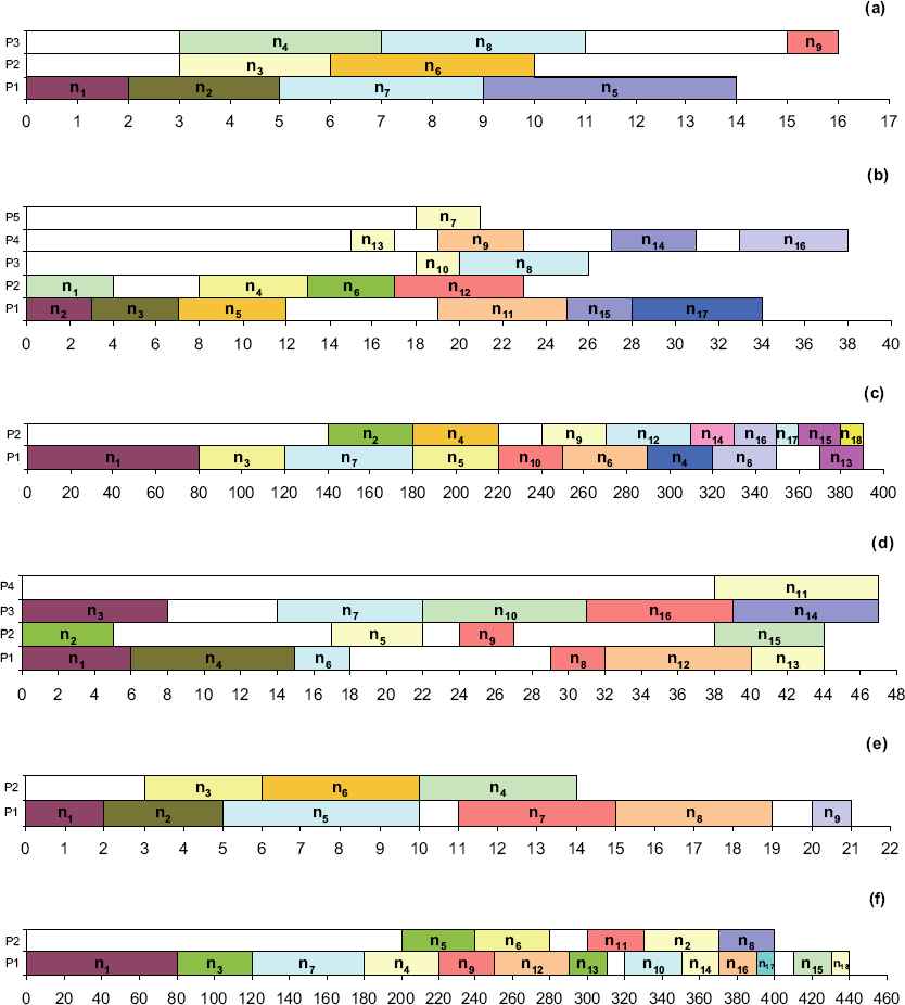
Achieved scheduling of six task graphs listed in Table 2 using the proposed approach. (a) G1 with nine tasks. (b) G2 with 17 tasks. (c) G3 with 18 tasks. (d) G4 with 16 tasks. (e) G5 with nine tasks. (f) G6 with 18 tasks.
| Graph | LC | EZ | MD | DSC | DCP | HLFET | ISH | ETF | LAST | MCP | DLS | ACO |
|---|---|---|---|---|---|---|---|---|---|---|---|---|
| G1 | 19 | 18 | 17 | - | 16 | 19 | 19 | 19 | 19 | 20 | 19 | 16 |
| G2 | 39 | 40 | 38 | 38 | 38 | 41 | 38 | 41 | 43 | 40 | 41 | 38 |
| G3 | 420 | 540 | 420 | 390 | 390 | 390 | 390 | 390 | 470 | 390 | 390 | 390 |
| G4 | - | - | - | - | - | 48 | - | 48 | - | 48 | 47 | 47 |
| G5 | - | - | 32 | 27 | 23 | 29 | - | 29 | - | 29 | 29 | 21 |
| G6 | - | - | 460 | 460 | 440 | 520 | - | 520 | - | 520 | 520 | 440 |
The last two graphs evaluate the proposed approach compared to the one of the best genetic algorithms proposed for multiprocessor task scheduling (without task duplication) [32]. Table 6 lists achieved results of not only these two algorithms but also four other traditional ones (for better justification). The results show the proposed approach with the genetic algorithm outperforms the other methods, yet the proposed approach has a better performance on the last graph. It should be noted that in this genetic algorithm, each generation has 100 chromosomes and the maximum number of generations is 1000, that is, it achieves its best scheduling by generating 100,000 solutions while the proposed approach examines only 1500 complete scheduling (1500 ants) to find its best answer. In other words, the proposed approach finds the solution faster than the genetic algorithm. It is logical because the ant colony optimization has an indirect communication by pheromone variables (Stigmergy) so that each new decision is based on the cumulative experience of all the previous ants.
| Graph | MCP | DSC | MD | DCP | Genetic | ACO |
|---|---|---|---|---|---|---|
| G5 | 29 | 27 | 32 | 32 | 23 | 21 |
| G6 | 520 | 460 | 460 | 440 | 440 | 440 |
The best achieved results of ACO-MTN, Genetic algorithm, and four traditional heuristics [32]
The last set of the experiments is conducted using random task graphs. Fig. 6 illustrates the achieved results (in NSL) for the proposed approach besides its traditional counterparts with respect to the different graph sizes. The entire 45 random task graphs are used, and the results are favored again the proposed approach. In addition, Fig. 7 shows the diagram of the achieved NSLs of the entire 45 random task graphs regarding utilization of the different number of processors. Again, the proposed approach outperforms the other methods by far in all the cases, and this confirms the prior experiments.
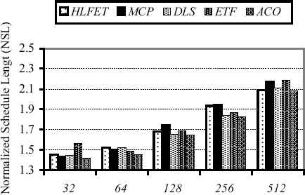
The achieved results (in NSL) of the proposed approach besides its traditional counterparts on the entire 45 random task-graphs with respect to the different graph sizes.
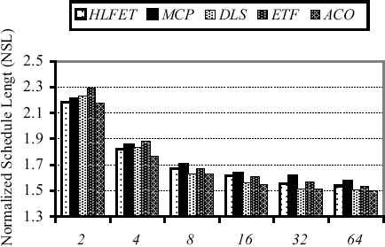
The diagram of the achieved NSLs of the entire 45 random task graphs regarding the different number of utilized processors.
6. Conclusion
In this paper, a new proposed approach based on ant colony optimization for multiprocessor task scheduling problem was introduced. The proposed approach is an iterative algorithm. In each iteration, an ant is created which finally produces a complete scheduling by assigning tasks to the processors using a probabilistic decision-making based on the dynamic pheromone variables and heuristics values (the priority measurement of the tasks). A set of experiments was conducted to specify the qualified priority measurement as heuristic values for each task. TLevel, BLevel, SLevel, ALAP, and NOO were considered, and finally the results showed that SLevel is more appropriate. Besides, six task graphs (G1–G6) were elected to evaluate the proposed approach against not only the traditional heuristics but also the genetic algorithm. Two sets of experiments were done to compare the proposed approach with traditional heuristics, one using a restricted number of processors (by two processor elements), and another using unbounded number of processors in order to interject the UNC approaches. The proposed method outperformed the heuristics in all the cases. In addition, another set of experiments on the last two graphs (G5 and G6) evaluated the proposed approach in comparison with one of the best genetic algorithms introduced to solve this problem. The proposed approach also outperformed the genetic algorithm. Furthermore, the aforementioned genetic algorithm examines about 100,000 solutions to achieve its best scheduling while the proposed approach considers only 1500 ones. In addition, the proposed approach was the winner of the race on a comprehensive set of 45 random task-graphs with different shape parameters such as size, CCR and the parallelism. All of these are of strong evidences to demonstrate the capability and superiority of the proposed approach in multiprocessor task-graph scheduling. Future work may be introducing a novel TDB approach based on ACO, and comparing and contrasting it versus the relevant methods.
Acknowledgements
Thanks to the reviewers for their useful comments, and Sama Technical and Vocational Training College, Islamic Azad University, Shoushtar Branch, for supporting this study as a research project.
Footnotes
Papadimitriou and Yannakakis
Duplication Scheduling Heuristics
Lowe Bound Algorithm
Bottom-up Top-down Duplication Heuristic
Linear Clustering with Task Duplication
Critical Path Fast Duplication
Michael-Jing-David
Duplication First and Reduction Next
Linear Clustering
Edge-Zeroing
Mobility Directed
Dominant Sequence Clustering
Dynamic Critical Path
Highest Level First with Estimated Time
Insertion Scheduling Heuristic
It uses the cluster-like CLANs to partition the task-graph
Localized Allocation of Static Tasks
Earliest Time First
dynamic Level Scheduling
Modified Critical Path
References
Cite this article
TY  - JOUR
AU  - Hamid Reza Boveiri
PY  - 2016
DA  - 2016/09/01
TI  - A Novel ACO-Based Static Task Scheduling Approach for Multiprocessor Environments
JO  - International Journal of Computational Intelligence Systems
SP  - 800
EP  - 811
VL  - 9
IS  - 5
SN  - 1875-6883
UR  - https://doi.org/10.1080/18756891.2016.1237181
DO  - 10.1080/18756891.2016.1237181
ID  - Boveiri2016
ER  -