
Analysis of Brand Image Effect on Advertising Awareness Using A Neuro-Fuzzy and A Neural Network Prediction Models
- DOI
- 10.2991/ijcis.2017.10.1.46How to use a DOI?
- Keywords
- Top of mind (TOM); share of voice (SOV); spontaneous awareness (SA); adaptive neuro-fuzzy inference system (ANFIS); artificial neural network (ANN)
- Abstract
Almost all the worldwide and nationwide companies utilize advertising to increase their sales volume and profit. These companies pay millions of dollars to reach consumers and announce their products or services. This forces companies to evaluate advertising effects and check whether ads meet companys strategies. They need to evaluate the ads not only after announcement, but also before advertising, i.e. they can be one step ahead by predicting the future advertising awareness through artificial intelligence tools such as fuzzy systems and neural networks. In this study, we propose to use adaptive neuro-fuzzy inference system (ANFIS) and artificial neural network (ANN) to analyze advertising decision making. ANFIS creates fuzzy rules and trains the neural network using given input data. This training ability of ANFIS and ANN leads to predicting the advertising awareness outputs. Here, we investigate three advertising awareness outputs, namely, top of mind, share of voice, and spontaneous awareness. In order to achieve the valid predictions, data are randomly divided into training data with 70 percent, validation data with 15 percent, and testing data with remained 15 percent of data. The correlation between actual data and predictions are calculated to check the accuracy of the predicted outputs.
- Copyright
- © 2017, the Authors. Published by Atlantis Press.
- Open Access
- This is an open access article under the CC BY-NC license (http://creativecommons.org/licences/by-nc/4.0/).
1. Introduction
Advertising originates in the history of ancient civilizations such as Romans’ paintings on the walls to announce gladiator fights, and sales announcements in Greece during golden age1. Today, companies exploit modern tools like social media to announce their activities and promote their products or services. Advertising nowadays covers a wide range of contents, from persuading people to purchase business products to educational messages and informing about healthcare services. The advent of internet and subsequently the emergence of social media has revolutionized the advertising formation. Searching for targeted audiences everywhere, companies form the structure of ads more psychologically professional and more tempting than predecessors. On the other hand, huge markets and vast advertising audiences encourage companies to expense hundreds of million dollars to advertise their brand in different media and stick their brand image in people’s mind. The huge costs of advertising and subsequent financial transactions represent the crucial role of advertising planning in today’s marketing management.
Lee and Johnson2 state that, in order for advertising planning, the advertising managers should review the marketing strategies to comprehend the company’s intentions, and then understand the role of advertising in the marketing mix. Advertisers should also perceive the current situation of the company, target market(s), short- and long-term marketing objectives, decisions on products’ life cycle, marketing mix, and their position in the market. This leads to clearly determining the advertising objectives of the company, and identify the precision and measurability of advertising. Therefore, advertiser would be able to evaluate advertising success at the end of the advertising campaign, and assess whether the advertising objectives would be met or not. Since advertising and then evaluation of advertising can be a time consuming and costly process, advertisers need to be one step ahead the trial and error, i.e. they should be able to predict the effect of a special advertising with particular advertising message. The prediction ability of artificial intelligence (AI) methods such as artificial neural networks (ANN) can suitably assist marketers to analyze the advertising success. These prediction methods are classified into two categories: linear and nonlinear 3. The first one, linear forecasting methods, such as least squares analysis or correlation methods are useful, but sometimes fail to forecast nonlinear time series. However, nonlinear prediction models such as ANN, ANFIS, Bayesian model, support vector regression, etc. provide effective performance in non-linear situation, and can effectively support advertisers.
The prediction ability of AI methods such as fuzzy systems or ANN can properly support advertiser. Using non-linear data of brand image components and its effect on advertising, non-linear prediction models can estimate the effects of advertising on brand or product awareness. This can elucidate the invisible side of advertising awareness and empower decision makers to estimate the consequences of their decisions. In this study, in order to rightly deal with non-linear and chaotic data, we apply ANN as well as ANFIS, which is a well-known combination of fuzzy inference systems (FIS) and ANN. We propose to utilize these methods to evaluate the effects of advertising on brand image through measuring the advertising metrics namely, top of mind (TOM), share of voice (SOV), and spontaneous awareness (SA).
This paper is structured as follows: Section 2 provides the literature review. Section 3 devotes to the advertising, advertising awareness and the influence of advertising on the brand image. The history of advertising and customer relationship, as well as the relevant concepts of advertising evaluation are presented in this section. Section 4 provides the analysis of brand image effects on advertising awareness. In this section, the methodologies including fuzzy sets, fuzzy rules, ANN, ANFIS, and finally the proposed model will be described. Section 5 contains the application of the proposed model and details of the given data. Ultimately, Section 6 is devoted to the conclusion and suggested future works.
2. Literature review
The complexity and non-linearity of the given data set is the main trouble of the most of the real data and time series. In order to analyze these data sets, AI methods offer many advantages over conventional statistical analysis like regression4. Neural network (NN) is a well-known AI method in dealing with outliers as well as incomplete, non-linear, and noisy data4. This interaction ability of NN catches many researchers from different disciplines to apply this method5. Most of these studies have used ANFIS and ANN from water management6 to prediction of brand awareness9.
Since marketing department of each company is in a direct relationships with customers, NN is suitably able to analyze the marketing studies through considering the intricate and large amount of customer insights to make proper predictions4. In this regard, Ho and Tsai7 used a neuro-fuzzy model to estimate the value innovation and the effects of quality of new product development (NPD) process on NPD performance. They compared the results of neuro-fuzzy model and structural equation modeling (SEM), and found the superiority of neuro-fuzzy model on SEM, due to effective explanation of nonlinear relationships between NPD process quality and NPD performance. Karahoca and Karahoca8 investigated the global service and mobile communication (GSM) for churn management using ANFIS method. Using x-means and fuzzy C-Means, they primarily clustered the input data, and then applied ANFIS for prediction. Lin et al.3 also developed a user interface as a geographic information system (GIS) to facilitate decision making process in telecommunication industry by comparing the performance of ANFIS, least squares analysis, logit analysis, and bass analysis.
Based on DeTienne and DeTienne’s4 claim that marketing studies can benefit from the ability of NNs to investigate customer preferences and customer satisfaction to make prediction. However NN is rarely applied to other applications of marketing such as advertising evaluation. For instance, Johansson and Niklasson9 used AI to estimate the advertising awareness in Swedish automotive market. By using ANN, TOM and in mind (IM) factors were predicted to measure the effect of advertising on 9 well-known automotive brands in Sweden9. Later, Johansson et al.10 employed NN and rule extraction to estimate TOM and IM of Swedish travel companies. But, to our knowledge, there are no more similar studies which employed ANFIS or ANN in advertising evaluation.
While AI methods are infrequently applied to marketing and advertising, they are frequently employed in other branches of management from stock market prediction to sales forecasting. By integrating ANN and fuzzy neural network, Kuo, Chen, and Hwang11 developed a DSS for stock trading. Atsalakis and Valavanis12 employed ANFIS to forecast short-term trends of Athens and New York stock markets. They chose Gaussian-2 shaped membership functions over bell-shaped Gaussian and triangular ones to fuzzify the system inputs, and found the lowest root mean square error. Esfahanipour and Aghamiri13 applied neuro-fuzzy inference adopted on a Tagaki-Sugeno-Kang to predict stock price and tested on the Tehran Stock Exchange Index (TEPIX). They used fuzzy C-Mean clustering method to identify the number of fuzzy rules. Using ANFIS, Boyacioglu and Avci14 predicted stock market return of Istanbul Stock Exchange (ISE). Ansari et al.15 used ANFIS to predict NASDAQ stock market index. This neuro-fuzzy system implemented hybrid least-square method and the back-propagation gradient descent methods to train the FIS. Esfahanipour and Mardani16 predicted Tehran stock exchange price index using multi-layer perceptron ANN and compared with ANFIS and fuzzy C-Means. Based on their prediction results, ANFIS outperformed ANN model with multi-layer perceptron. Svalina et al.17 applied neuro-fuzzy inference system to predict Zagreb Stock Exchange Crobex index.
Kuo and Xue18 and Kuo and Xue19 implemented a decision support system (DSS) and employed fuzzy ANN and ANN to forecast sales volume. Using fuzzy Delphi method to collect the fuzzy inputs and outputs, fuzzy if-then rules, achieved from marketing experts, were trained and then integrated into the forecast from ANN. Kuo20 proposed a fuzzy ANN model to train fuzzy if-then rules to forecast sales data. This system was initialized with generated weights by genetic algorithm. Afterwards, based on this integrated model, Kuo, Chen, and Hwang21 developed a DSS for stock trading. Kuo, Wu, and Wang11, then, boosted the integrated ANN and fuzzy ANN system by adding fuzzy weight elimination. Ustundag22 used three methods including fuzzy rule-based system, ANN, and ANFIS to predict product sales of the largest Turkish paint producer. Efendigil, Onut, and Kahraman23 employed ANN and ANFIS to forecast demand of a multilevel supply chain. In this study, the results of ANFIS were closer to the actual values than the results of ANN. Berneti 24 combined ANFIS and imperial competitive algorithm to forecast the produced oil of 31 wells in the northern Persian Gulf field of Iran. Dwivedi, Niranjan, and Sahu25 also applied ANFIS and ANN to forecast the automobile sales, which resulted ANFIS outperformance.
These huge number of NN applications to solve management troubles represent the growing popularity of AI methods in managerial contexts. As you see in studies above, ANFIS or ANN or other estimation methods are not absolutely superior to each other. However, each of these methods outperform the other in different situations. On the other hand, as mentioned before, advertising is the cornerstone of marketing strategies which is difficult to be evaluated26. This demonstrates the significance and complexity of the elements of advertising evaluation, which can unveil non-linear relationships between the elements. Consequently, considering the abilities of AI methods such as fuzzy systems or NN in dealing with non-linear and complex data, these methods can provide practical and useful outcomes in advertising evaluation problems.
3. Brand image and advertising awareness
According to Kotler and Armstrong1, psychological theories enumerate four main factors which influence a person’s purchase decision, namely motivation, perception, learning, and beliefs and attitudes. Motivation represents the need that sufficiently press the person to buy the product or service and satisfy the need. A motivated person perceives the process of selection, organizing, and interpreting information to form a meaningful picture of the world. This perception leads to changes in an individual’s behavior and learn from experiences. Finally, the learning process terminates to create the last factor beliefs and attitudes.
Marketers consider these beliefs of people to supply their needed products or services5. They firstly create a brand which is a name, term, sign, symbol, or a combination of these elements to introduce the product or service1, and then develop an influential image of the brand that affects buying behavior. The beliefs and attitudes later shape the brand image in the mentality of consumers. According to Keller27, brand image is formed by a set of perceptual beliefs regarding a brand’s attribute, benefit, and attitude associations, which are frequently seen as the basis for a general evaluation of the brand or attitude toward it27. Brand image is a holistic construct formed from a gestalt of all the brand associations related to the brand. Brand attitude, which is consumers’ overall evaluation of the brand, is the other forming component of the brand image. However, brand attitude is conceptualized as just one of the various associations used in the formation of the brand image.
In general, brand image is considered as a combination of brand associations, brand loyalty, brand awareness, perceived quality, and other brand assets27,28. As represented in Figure 1, the ultimate construct of this chain, brand equity, is defined as a behaviorally oriented construct influenced by a consumer’s image and attitude of the behavior’s object28.
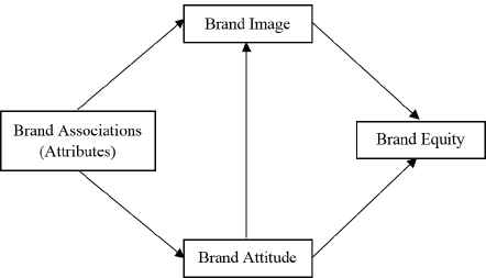
Brand associations, brand image, brand attitude, and brand equity.
Nowadays, almost all business companies use advertising to create brand awareness and/or product awareness, and promote their products. Kotler and Armstrong1 states that advertising strategy includes (1) creating message and (2) selecting appropriate media. The first step, advertising message, refers to a communication way to consumers, which should get consumers to think about or react to the product or company in advertiser’s determined way1. Secondly, selecting advertising media refers to determining reach, frequency, and impact of advertisement. The marketing department should make decision on the media type, media vehicles, and media timing. People react to the advertising only if they believe they will benefit from the presented product or service. The message of advertisement tends to plain, straightforward outlines of benefits and positioning points that the advertiser wants to stress1.
Advertising is often the largest single cost in marketing budget and companies are giving weight to advertising research5. Similar to Kotler and Armstrong’s1 advertising strategy, Lee and Johnson2 described advertising research by dividing it into two categories: (1) message research and (2) media research. Message research concerns the effectiveness of advertising message in communicating to people, and addresses how well those messages influence people’s behavior. However, media research analyzes the circulation of information in newspapers and magazines, and broadcast coverage of television and radio.
Measuring advertising effectiveness and the return on advertising investment has become a crucial subject for most companies which are challenging in the current competitive economic environment5. Considering advertising effectiveness, advertising researchers measure the changes of people’s attitudes, awareness, copy points, emotional responses, and purchase choices. In order to develop an objective methods for advertising evaluation, marketers come to a conclusion on measuring the effects of advertising through (1) the sales and profit effects, and (2) the communication effects of advertising1.
The sales and profit effects of advertising can be regarded by comparing the post-advertising sales and profits with pre-advertising sales and profits. The drawback of this method is to find the appropriate measurement time before, and especially after advertising. On the other hand, the communication effects can be evaluated by observation of consumers’ recall after running an advertising. Similar to the sales and profit effects measurement, the effects of pre-advertising and post-advertising communications will reveal the advertising awareness. This measurement requires the link between consumer, customer, and public to the marketer. The stream of information can identify and reveal marketing opportunities, which leads to generating appropriate marketing actions. Hence, although it is not easy to track the incremental sales or recall associated with advertising campaigns, marketers have developed a number of marketing metrics such as TOM, SOV, SA, and IM, which the first three ones are considered in this study.
3.1. TOM
TOM evaluates the advertising awareness, which represents the first brand that comes to mind when a respondent is asked an unprompted question about a category. TOM is measured as the percentage of respondents for whom a given brand is top of their mind26. Using TOM, marketers can evaluate the influence of the transmitted advertising, i.e. if an advertising successfully received to audiences, it should stick in top of their minds.
3.2. SOV
SOV is an advertising awareness metric which refers to the intensity of advertising for a particular brand compared with all other brands of a given market. It is generally measured in dollars, and can be calculated at a company level, brand level, or product level26,29. Farris et al.26 defines SOV as the amount of advertising of a company compared to that of its competitors, i.e. SOV quantifies the advertising presence that a specific brand exploits. The percentage of SOV is calculated as follows:
3.3. SA
According to Maketing Research Association30, SA points out the remembrance of a brand name by a respondent. The percentage of people who mention a particular brand forms the SA of that brand. The difference between TOM and SA is that TOM concerns with the first brand mentioned by respondent, but SA regards the entire memorized brands, no matter the first or the last5.
4. Analysis of Brand Image Effect on Advertising Awareness
As mentioned before, the proposed model employs ANFIS and ANN. ANFIS is an integration of fuzzy inference systems (FIS) and neural networks (NN). FIS refers to a knowledge expression system which uses linguistic rules. NN is also a well-known data-driven training system. These methods naturally carry certain drawbacks that reduce their performances. However, according to Abraham31, FIS and ANN are complementary methods that their combination can resolve the drawbacks pertaining to them. The term neuro-fuzzy denotes to applying the NN to fuzzy inference systems32. From the viewpoint of FIS, learning ability of NN is an advantage, and accordingly, from the viewpoint of ANN, the formation of linguistic rules will be another advantage31. These terms are briefly introduced in the following part and then the proposed model will be given.
4.1. FIS
Maybe the most powerful form of conveying information is natural language during reasoning or problem solving33. This led Zadeh34 to defining a linguistic variable as a variable which values are words or sentences in a natural or artificial language. Linguistic variables facilitate the expression of human reasoning and extract the latent knowledge of experts. According to Negnevisky35, knowledge is ”a theoretical or practical understanding of a subject or a domain”. Although it is difficult to represent the knowledge of experts in the form of algorithms, artificial intelligence provides various ways to represent knowledge 35. Perhaps the most common way to express human knowledge is to form it into if-then fuzzy rules. The fuzzy level of understanding and describing an FIS is expressed in the form of a set of restrictions on the output based on certain conditions of the input. Conjunctions or disjunctions like ”and”, ”or”, and/or ”else” are the restrictions of rules that connect different linguistic expressions to create more complex premise.
Conjunctive system of rules like y = y1 and y2 and ... and yr which is defined by the membership function (MF) is as follows:
Disjunctive system of rules like y = y1 or y2 or ... or yr which is defined by MFs is as follows:
These rules or complex rules by conjunction or disjunction of them form the rule base of an FIS. This rule base will be used by NN to make learning process.
4.2. NN
A NN is an attempt of modeling human cognitive system to overcome the restrictions of traditional computers. NN has been mainly applied to prediction, clustering, classification, and alerting to abnormal patterns40. NNs can identify patterns between the dependent and independent variables in datasets. This pattern recognition as well as optimization of large-scale problems are the principal strengths of ANNs4,36. The advantages of NNs are its effective interaction with data discontinuities, outliers, missing data and nonlinear transformations. However, NN is notorious for its complex computations. The other main disadvantage of NN is the restriction of the number of hidden neurons which hinders the function of NN.
NN is typically composed of three major layers including input layer, hidden layer, and output layer, which each has several highly interconnected computational units called neurons or nodes. In a prediction application of NN, the number of independent variables determines the number of input nodes, and the number of output nodes is specified by predicted variables. According to some studies, the number of hidden layer nodes can be up to (1) 2n + 1 (where n is the number of nodes in the input layer), (2) 75% of the number of input nodes, or (3) 50% of the number of input and output nodes23,37,38,39.
Figure 2 depicts the topology of NN and represents the hidden neurons bridge the input and output neurons, and play the computational role in the NN as follows:
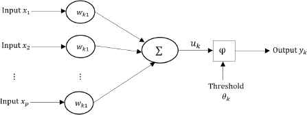
Non-linear model of a neuron.
Function φ in the Eq. (5) is the AF which limits the neuron’s output to a range, usually between 0 and 1, or −1 and 1. It can be either linear or nonlinear. Linear AF allows a multi-layer network to be represented as a single-layer network, and nonlinear AF transfers information between layers in ways that allow new modeling capabilities 4. Following sigmoid or logistic function is the most popular AF for back-propagation NN.
In back-propagation NN, the errors resulting from the comparison of the actual and target output values are propagated backward through the network, and the weight values are adjusted to minimize error. The training process will stop when all patterns are classified correctly and selected a range of accuracy. This is called over-fitting or over-training. The objective function of NN is the minimization of squared error as follows:
4.3. Adaptive Neuro-Fuzzy Inference System
Among neuro-fuzzy studies, Wang42 proposed the singleton type neuro-fuzzy model in which an analytical expression is obtained for the output of the system versus the inputs are implemented by a NN23. As mentioned before, the main feature of this model is that the number of input membership functions (fuzzy sets) is equal to the number of rules providing ease in implementation. Palit and Babuska43 later modified Wang’s42 model to Takagi-Sugeno (TS) type of neuro-fuzzy model. This TS model has been called adaptive network-based fuzzy inference system or briefly ANFIS, which has been broadly established in time-series predictions and system identification.
ANFIS44 implements a Takagi-Sugeno FIS and has a five layered architecture as shown in Figure 3. The first hidden layer is for fuzzification of the input variables and T-norm operators are deployed in the second hidden layer to compute the rule antecedent part. The third hidden layer normalizes the rule strengths followed by the fourth hidden layer where the consequent parameters of the rule are determined. Output layer computes the overall input as the summation of all incoming signals. ANFIS uses back-propagation learning to determine premise parameters (to learn the parameters related to membership functions) and least mean square estimation to determine the consequent parameters.
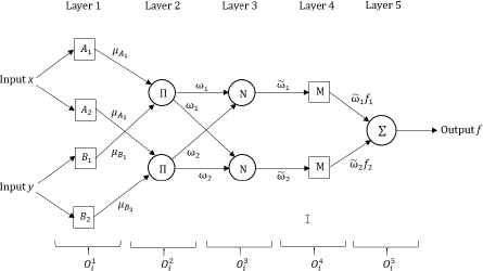
The architecture of ANFIS.
As shown in Figure 3, ANFIS has a five-layered architecture. The first layer receives the input MFs (fuzzy sets). The quantity of inputs is equal to the number of rules23. After fuzzification of the rules by the first layer, the second layer deploys the T-norm operators to calculate the rule antecedent part. The third layer normalizes the rule strengths, and the fourth layer determines the consequent parameters of the rule. Finally, the output layer computes the overall input as the summation of all incoming signals. ANFIS applies back-propagation to learn the parameters related to membership functions (premise parameters), and uses least mean square estimation to determine the consequent parameters31.
As a neuro-fuzzy system, ANFIS has obviously two components: (1) FIS and (2) ANN. The inference system create the fuzzy rules and then ANN trains the rules to find the optimal output. The FIS constructs an input-output mapping based on human knowledge in the form of fuzzy if-then rules with appropriate membership functions and stipulated input-output data pairs23 with two inputs x and y, and one output z.
- •
Rule I: If x is A1 and y is B1, then z = f1 = p1x + q1y + r1
- •
Rule II: If x is A2 and y is B2, then z = f2 = p2x + q2y + r2
ANFIS then applies an NN to determine the shape of membership functions and extract rule. The mathematical process of the five layers of ANFIS are described as follows:
Layer 1. Every node i in this layer is a square node with a node function.
where x denotes the input to node i, and Ai is the linguistic label like small, large, etc. Oi is the membership function of Ai and it specifies the degree to which the given x satisfies the quantifier Ai. The membership function can be triangular, trapezoidal, bell-shaped, Gaussian, etc.where ai, bi, ci is the parameter set of the bell-shaped membership function.Layer 2. Every node in this layer is a circle node labeled ∏ which multiplies the incoming signals and sends the product out. For instance,
Each node output represents the firing strength of a rule.
Layer 3. Every node in this layer calculates the ratio of the ith rule’s firing strength to the sum of all rules’ firing strengths:
The output of this layer is called normalized firing strengths.
Layer 4. Every node i in this layer is a square node with a node function
where pi, qi, ri is the parameter set which are referred to as consequent parameters.Layer 5. The single node of this layer calculates the overall output as a summation of all incoming signals as follows:
In ANFIS structure, the premise and consequent parameters should be noted as important factors for the learning algorithm in which each parameter is utilized to calculate the output data of the training data. The premise part of a rule defines a subspace, while the consequent part specifies the output within this fuzzy subspace45.
Given the values of premise parameters, the overall output can be expressed as linear combinations of the consequent parameters. According to Jang45, the output of ANFIS can be as below:
Using fuzzy if-then rules and Eq. (15), Eq. (16) will be yielded as follows:
After arrangement, Eq. (16) becomes
4.4. The Proposed Model
The steps of the proposed model are given in the following:
Step 1. Enter the brand image variables as inputs and an advertising awareness metric as output variable.
If too many input variables are given, principle component analysis (PCA) can be used to reduce the size of the problem.
Step 2. Determine input and output data and split data to training, validation, and testing datasets.
Step 3. Make prediction.
The learning process will be conducted epoch by epoch and should be stopped when the error of training dataset sticks in a minimum.
Step 3.1. Prediction using ANN.
Step 3.1.1. Find the optimal architecture of NN using training and validation datasets, and determine the weights of hidden layers.
Step 3.1.2. Optimize the weights of hidden layer through back-propagation.
Step 3.1.3. Use activation function and sum up the output to predict the advertising awareness metric.
Step 3.2. Prediction using ANFIS.
Step 3.2.1. Form the fuzzy rule base using brand image inputs and advertising awareness output variables such that
Rule I) If brand reputation is A1 and advertising cost is B1, then TOM = f1 = P1A1 + Q1B1 + R1
Rule II) If brand reputation is A2 and advertising cost is B2, then TOM = f2 = P2A2 + Q2B2 + R2
Step 3.2.2. Determine the parameters Pi, Qi, Ri and calculate the antecedent and consequent of rules.
Step 3.2.3. Optimize the parameters and find the optimal brand image inputs and advertising awareness output.
Step 3.2.4. Defuzzify the rules by aggregating the advertising awareness output and predict the advertising awareness output.
Step 4. Compare the error of actual data and predictions of ANN and ANFIS.
As shown in Figure 4, the flowchart of the proposed model depicts the steps of the proposed model, and illustrate the stream of data and the calculations to find the final prediction of the output variable.
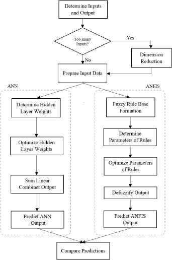
The flowchart of the proposed model.
Figure 5 represents the network of the proposed model with n inputs of brand image components and a single advertising awareness output. The upper part of the network shows the layers of ANFIS and the lower part demonstartes the layers of ANN.
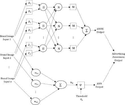
The network of the proposed model.
5. Application
The proposed model applies ANFIS and ANN to evaluate the effect of brand image on advertising awareness data of fifteen prominent Turkish companies from different sectors. In order to analyze the data of homogenous brands together, given companies are classified into two groups: companies which produce fast moving consumer goods (FMCG), and on the other side, non-FMCG producers. We will check if this classification makes any contribution in prediction of brand image effects on advertising awareness.
In future parts, ”all data” refers to the data of all brands which are pooled and analyzed together. ”FMCG data” means the pooled data of 7 FMCG brands, and the data of remained 8 brands are called ”non-FMCG data”. And as mentioned in Section 3, we consider TOM, SOV, and SA as the advertising awareness metrics, and predict their values.
5.1. Data Description
The dataset includes the results of a field study on advertising awareness, which is gathered by questionnaire during 21 months, from January 2014 to September 2015. The questionnaire covers 30 questions about the components of brand image and advertising awareness.
The questions extract people’s awareness on the advertising of fifteen reputable Turkish brands. Here, we cannot mention these brands because of the confidentiality of their advertising information.
In addition to 30 input variables, gross rating point (GRP), which is the advertising costs of each company, is also considered as the 31th input variable. These variables are determined as inputs of ANFIS method; however, since running of ANFIS with 31 input variables is almost impossible and requires a high-performance supercomputer, we employed PCA for dimension reduction. We firstly excluded GRP and then applied PCA to the remained 30 input variables, which its results are presented in Tables 1 and 2.
| KMO Measure of Sampling Adequacy | 0.979 | |
| Bartlett’s Test of Sphericity | Approx. Chi-Square | 13665.883 |
| df | 435 | |
| Sig. | 0.000 |
Kaiser-Meyer-Olkin (KMO) and Bartlett’s test.
| Component | Initial Eigenvalues | ||
|---|---|---|---|
| Total | % of Variance | Cumulative % | |
| 1 | 21.667 | 72.223 | 72.223 |
| 2 | 2.338 | 7.793 | 80.016 |
| 3 | 0.724 | 2.414 | 82.431 |
| 4 | 0.610 | 2.033 | 84.464 |
| 5 | 0.439 | 1.464 | 85.928 |
| 6 | 0.356 | 1.186 | 87.114 |
| 7 | 0.347 | 1.157 | 88.271 |
| 8 | 0.305 | 1.018 | 89.289 |
| 9 | 0.268 | 0.894 | 90.183 |
| 10 | 0.249 | 0.830 | 91.013 |
| 11 | 0.228 | 0.762 | 91.774 |
| 12 | 0.218 | 0.726 | 92.501 |
| 13 | 0.202 | 0.674 | 93.174 |
| 14 | 0.194 | 0.647 | 93.821 |
| 15 | 0.177 | 0.590 | 94.412 |
| 16 | 0.170 | 0.568 | 94.980 |
| 17 | 0.156 | 0.519 | 95.498 |
| 18 | 0.143 | 0.476 | 95.974 |
| 19 | 0.134 | 0.448 | 96.422 |
| 20 | 0.130 | 0.434 | 96.856 |
| 21 | 0.124 | 0.413 | 97.269 |
| 22 | 0.113 | 0.377 | 97.646 |
| 23 | 0.108 | 0.359 | 98.005 |
| 24 | 0.104 | 0.345 | 98.350 |
| 25 | 0.096 | 0.320 | 98.670 |
| 26 | 0.092 | 0.307 | 98.977 |
| 27 | 0.088 | 0.292 | 99.269 |
| 28 | 0.081 | 0.272 | 99.541 |
| 29 | 0.071 | 0.237 | 99.777 |
| 30 | 0.067 | 0.223 | 100.000 |
Total variance explained by PCA of given inputs.
As shown in Table 1, KMO measure of sampling adequacy is 0.979 which is greater than 0.900, so the sample size is marvelous. Since Bartlett’s test of sphericity is 0.000, which is less than 0.005, null hypothesis is rejected and the correlation matrix of variables is not an identity matrix. This means there would be correlations between the variables. As represented in Table 2, two components reach eigenvalues greater than 1.000, and they can explain more than 80 percent of total variance, which is a very good result. Finally, PCA reduced the number of variables to 2, factor1 and factor2. Using these two components along with GRP as the inputs of the proposed model, we separately predicted TOM, SOV, and SA variables as outputs of the proposed model.
5.2. ANFIS Architecture
Given data is divided into training, validation, and testing datasets with 70, 15, and 15 percent division ratios which is the default of the neural network tool-box of MATLAB 46, and frequently used division ratios 47.
Running ANFIS by above-mentioned input and output variables, we calculated the least validation errors and found the most appropriate fuzzy MF and the number of MFs in each fuzzy envelope. Here, the fuzzy MFs include triangular-shaped-built-in MF, trapezoidal-shaped-built-in MF, generalized bell-shaped built-in MF, and Gaussian curve built-in MF, with 3, 5, and 7 MFs. To obtain Tables 3, 4, and 5, data are devided into training, validation, and testing sets, and the errors of ANFIS predictions are represented for all, FMCG, and non-FMCG datasets, respectively.
| Output Type | MF Type | Number of MFs | Constant | Linear | ||||
|---|---|---|---|---|---|---|---|---|
| Training Error | Validation Error | Testing Error | Training Error | Validation Error | Testing Error | |||
| TOM | Triangular | 3 | 0.0296 | 0.0862 | 0.0612 | 0.0278 | 0.2466 | 0.3839 |
| 5 | 0.0272 | 0.4064 | 0.0780 | 0.0240 | 10.6639 | 13.4414 | ||
| 7 | 0.0245 | 0.3293 | 0.1726 | 0.0152 | 23.4523 | 13.1794 | ||
| Trapezoidal | 3 | 0.0305 | 0.0483 | 0.0396 | 0.0279 | 0.1150 | 0.0665 | |
| 5 | 0.0275 | 0.0644 | 0.0449 | 0.0240 | 0.0887 | 0.4451 | ||
| 7 | 0.0248 | 0.0663 | 0.0726 | 0.0139 | 0.4187 | 0.3942 | ||
| Bell-shaped | 3 | 0.0291 | 0.0506 | 0.0430 | 0.0272 | 1.3070 | 0.3138 | |
| 5 | 0.0254 | 3.5696 | 0.6040 | 1.6369 | 742.2224 | 366.9662 | ||
| 7 | 0.0195 | 1.2579 | 0.5148 | 1.3611 | 694.0294 | 529.3226 | ||
| Gaussian | 3 | 0.0292 | 0.0557 | 0.0406 | 0.0261 | 0.3264 | 0.3123 | |
| 5 | 0.0264 | 0.7384 | 0.2294 | 0.1159 | 711.1120 | 266.2938 | ||
| 7 | 0.0195 | 3.3175 | 0.1955 | 0.2456 | 674.5820 | 289.0860 | ||
| SOV | Triangular | 3 | 0.0165 | 0.0491 | 0.0342 | 0.0142 | 0.5169 | 0.4846 |
| 5 | 0.0107 | 1.2040 | 0.1500 | 0.0084 | 4.9665 | 5.0288 | ||
| 7 | 0.0054 | 0.1889 | 0.0882 | 0.0035 | 2.6694 | 1.0607 | ||
| Trapezoidal | 3 | 0.0264 | 0.0405 | 0.0406 | 0.0125 | 0.0625 | 0.1292 | |
| 5 | 0.0176 | 0.1323 | 0.0442 | 0.0116 | 0.0466 | 0.0807 | ||
| 7 | 0.0132 | 0.0645 | 0.0453 | 0.0034 | 0.1661 | 0.2947 | ||
| Bell-shaped | 3 | 0.0151 | 0.0854 | 0.0353 | 0.0108 | 2.9423 | 1.0706 | |
| 5 | 0.0111 | 0.0423 | 0.0659 | 0.3709 | 70.9768 | 104.0837 | ||
| 7 | 0.0077 | 0.6858 | 0.1644 | 0.1913 | 361.4856 | 78.7972 | ||
| Gaussian | 3 | 0.0165 | 0.4053 | 0.0517 | 0.0101 | 1.2462 | 0.3467 | |
| 5 | 0.0101 | 0.0667 | 0.0849 | 0.0211 | 270.0354 | 371.2678 | ||
| 7 | 0.0062 | 0.1967 | 0.1415 | 0.0116 | 144.5780 | 62.6204 | ||
| SA | Triangular | 3 | 0.0183 | 0.0328 | 0.0303 | 0.0162 | 0.1121 | 0.2742 |
| 5 | 0.0159 | 0.5394 | 0.1217 | 0.0131 | 4.4640 | 5.4319 | ||
| 7 | 0.0139 | 0.1768 | 0.1592 | 0.0213 | 16.9450 | 6.9059 | ||
| Trapezoidal | 3 | 0.0186 | 0.0214 | 0.0193 | 0.0165 | 0.0377 | 0.0321 | |
| 5 | 0.0167 | 0.0412 | 0.0386 | 0.0137 | 0.6144 | 0.0886 | ||
| 7 | 0.0153 | 0.0313 | 0.0655 | 0.0079 | 0.4097 | 0.3973 | ||
| Bell-shaped | 3 | 0.0172 | 0.0398 | 0.0232 | 0.0153 | 1.2523 | 0.3653 | |
| 5 | 0.0139 | 0.8724 | 0.2881 | 0.3284 | 204.1255 | 358.0230 | ||
| 7 | 0.0116 | 0.5974 | 0.3084 | 0.2859 | 584.2076 | 143.1140 | ||
| Gaussian | 3 | 0.0182 | 0.0250 | 0.0186 | 0.0146 | 0.2011 | 0.1697 | |
| 5 | 0.0149 | 0.8844 | 0.1937 | 0.0809 | 126.1488 | 478.2682 | ||
| 7 | 0.0119 | 0.2930 | 0.2225 | 0.0835 | 377.5020 | 93.6148 | ||
Training, validation and testing errors of ANFIS using all data.
| Output Type | MF Type | Number of MFs | Constant | Linear | ||||
|---|---|---|---|---|---|---|---|---|
| Training Error | Validation Error | Testing Error | Training Error | Validation Error | Testing Error | |||
| TOM | Triangular | 3 | 0.0226 | 0.0733 | 0.0477 | 0.0158 | 3.3890 | 2.7278 |
| 5 | 0.0159 | 0.1146 | 0.0644 | 0.0084 | 3.9211 | 2.6235 | ||
| 7 | 0.0095 | 1.2427 | 0.0691 | 0.0002 | 7.6118 | 3.7490 | ||
| Trapezoidal | 3 | 0.0249 | 0.0414 | 0.0526 | 0.0175 | 0.0909 | 0.0320 | |
| 5 | 0.0182 | 0.0835 | 0.0516 | 0.0104 | 0.2782 | 0.5347 | ||
| 7 | 0.0109 | 0.3938 | 2.9011 | 0.0004 | 1.6489 | 11.5608 | ||
| Bell-shaped | 3 | 0.0189 | 0.0990 | 0.0438 | 0.0106 | 1.0550 | 5.0596 | |
| 5 | 0.0094 | 0.9054 | 1.1287 | 0.4494 | 691.7222 | 273.6307 | ||
| 7 | 0.0049 | 0.9488 | 0.2171 | 0.0088 | 24.1414 | 6.0147 | ||
| Gaussian | 3 | 0.0201 | 0.0632 | 0.0344 | 0.0111 | 3.0306 | 16.3693 | |
| 5 | 0.0100 | 0.7203 | 0.9491 | 0.6991 | 2170.9207 | 704.0659 | ||
| 7 | 0.0062 | 0.0754 | 0.0817 | 0.0003 | 10.5565 | 7.6864 | ||
| SOV | Triangular | 3 | 0.0194 | 0.0377 | 0.0406 | 0.0174 | 7.1962 | 5.0368 |
| 5 | 0.0114 | 0.3918 | 0.1884 | 0.0030 | 4.1225 | 1.5774 | ||
| 7 | 0.0045 | 1.1392 | 0.5975 | 0.0017 | 10.4856 | 5.4835 | ||
| Trapezoidal | 3 | 0.0308 | 0.0421 | 0.0352 | 0.0100 | 0.1647 | 0.0597 | |
| 5 | 0.0198 | 0.0762 | 0.1243 | 0.0087 | 0.1185 | 0.1001 | ||
| 7 | 0.0167 | 0.0993 | 0.0639 | 0.0005 | 1.4907 | 12.4801 | ||
| Bell-shaped | 3 | 0.0168 | 0.1836 | 0.1401 | 0.0075 | 1.5793 | 4.0190 | |
| 5 | 0.0094 | 1.5388 | 0.6144 | 0.0829 | 227.2386 | 93.1308 | ||
| 7 | 0.0032 | 0.2231 | 0.1228 | 0.0016 | 57.3140 | 1.4133 | ||
| Gaussian | 3 | 0.0192 | 0.2328 | 0.2322 | 0.0096 | 4.2788 | 23.1572 | |
| 5 | 0.0084 | 0.5223 | 1.6871 | 0.0203 | 329.9985 | 173.8375 | ||
| 7 | 0.0032 | 0.2174 | 0.0745 | 0.0005 | 27.4781 | 1.7122 | ||
| SA | Triangular | 3 | 0.0185 | 0.0379 | 0.0333 | 0.0158 | 4.0985 | 2.8782 |
| 5 | 0.0148 | 0.2622 | 0.1304 | 0.0077 | 51.6586 | 18.6790 | ||
| 7 | 0.0093 | 0.3516 | 0.2849 | 0.0005 | 15.7653 | 6.6216 | ||
| Trapezoidal | 3 | 0.0176 | 0.0201 | 0.0339 | 0.0142 | 0.1496 | 0.0337 | |
| 5 | 0.0175 | 0.0378 | 0.0391 | 0.0075 | 0.2671 | 0.0730 | ||
| 7 | 0.0130 | 0.2339 | 2.7914 | 0.0001 | 3.8759 | 3.5350 | ||
| Bell-shaped | 3 | 0.0150 | 0.1492 | 0.0765 | 0.0112 | 0.3418 | 1.6063 | |
| 5 | 0.0085 | 0.4941 | 0.9300 | 0.2039 | 563.7178 | 420.4108 | ||
| 7 | 0.0024 | 0.4895 | 0.1780 | 0.0029 | 39.5024 | 2.4692 | ||
| Gaussian | 3 | 0.0167 | 0.0194 | 0.0530 | 0.0115 | 1.8937 | 7.4270 | |
| 5 | 0.0076 | 0.5871 | 0.1362 | 0.0717 | 584.7540 | 58.0627 | ||
| 7 | 0.0057 | 0.7674 | 0.2415 | 0.0002 | 22.7041 | 2.8330 | ||
Training, validation and testing errors of ANFIS using FMCG data.
| Output Type | MF Type | Number of MFs | Constant | Linear | ||||
|---|---|---|---|---|---|---|---|---|
| Training Error | Validation Error | Testing Error | Training Error | Validation Error | Testing Error | |||
| TOM | Triangular | 3 | 0.0260 | 0.0487 | 0.0686 | 0.0158 | 0.1974 | 0.4058 |
| 5 | 0.0175 | 1.9572 | 0.8235 | 0.0151 | 372.8480 | 39.5400 | ||
| 7 | 0.0065 | 1.1458 | 0.4814 | 0.0009 | 35.2356 | 8.5340 | ||
| Trapezoidal | 3 | 0.0258 | 0.0345 | 0.0395 | 0.0194 | 1.6025 | 0.2842 | |
| 5 | 0.0217 | 0.0745 | 0.0744 | 0.0069 | 0.7779 | 1.1840 | ||
| 7 | 0.0152 | 0.1617 | 0.0711 | 0.0011 | 11.0772 | 0.2474 | ||
| Bell-shaped | 3 | 0.0234 | 0.5689 | 0.0791 | 0.0170 | 3.2345 | 1.9166 | |
| 5 | 0.0173 | 2.6659 | 0.8162 | 0.1661 | 516.9710 | 208.1357 | ||
| 7 | 0.0059 | 0.2969 | 0.2995 | 0.0011 | 15.4259 | 6.2004 | ||
| Gaussian | 3 | 0.0254 | 0.0698 | 0.1274 | 0.0157 | 2.6489 | 0.3540 | |
| 5 | 0.0171 | 1.8812 | 0.4854 | 0.0315 | 396.7359 | 278.2561 | ||
| 7 | 0.0064 | 1.6977 | 0.3474 | 0.0009 | 22.1566 | 10.4615 | ||
| SOV | Triangular | 3 | 0.0065 | 0.0317 | 0.0396 | 0.0048 | 0.3467 | 0.2479 |
| 5 | 0.0036 | 0.1356 | 0.4022 | 0.0021 | 17.3201 | 10.9000 | ||
| 7 | 0.0017 | 0.2331 | 0.1462 | 0.0000 | 2.4780 | 1.7347 | ||
| Trapezoidal | 3 | 0.0112 | 0.0425 | 0.0194 | 0.0043 | 0.6245 | 0.0311 | |
| 5 | 0.0067 | 0.0703 | 0.0767 | 0.0002 | 0.1319 | 0.2828 | ||
| 7 | 0.0023 | 0.1743 | 0.0315 | 0.0000 | 1.8185 | 0.0518 | ||
| Bell-shaped | 3 | 0.0061 | 0.0441 | 0.0641 | 0.0031 | 0.9307 | 0.6136 | |
| 5 | 0.0023 | 0.0921 | 0.1034 | 0.0175 | 89.7381 | 15.6011 | ||
| 7 | 0.0006 | 0.1751 | 0.1262 | 0.0002 | 1.2702 | 1.1269 | ||
| Gaussian | 3 | 0.0064 | 0.0323 | 0.0612 | 0.0030 | 0.4146 | 0.2321 | |
| 5 | 0.0025 | 0.1908 | 0.1023 | 0.0074 | 31.2400 | 41.5864 | ||
| 7 | 0.0008 | 0.1921 | 0.0857 | 0.0001 | 1.0284 | 0.6115 | ||
| SA | Triangular | 3 | 0.0140 | 0.0396 | 0.0266 | 0.0110 | 0.3262 | 0.2249 |
| 5 | 0.0109 | 0.3777 | 0.1041 | 0.0110 | 286.8446 | 20.1561 | ||
| 7 | 0.0071 | 0.4168 | 0.2382 | 0.0005 | 20.4992 | 4.3428 | ||
| Trapezoidal | 3 | 0.0149 | 0.0250 | 0.0184 | 0.0114 | 1.8445 | 0.1943 | |
| 5 | 0.0121 | 0.0540 | 0.0514 | 0.0052 | 0.3453 | 0.2158 | ||
| 7 | 0.0103 | 0.9797 | 0.0402 | 0.0012 | 4.0176 | 0.2092 | ||
| Bell-shaped | 3 | 0.0136 | 0.0389 | 0.0218 | 0.0105 | 0.8227 | 1.4813 | |
| 5 | 0.0078 | 0.7034 | 0.2616 | 0.0308 | 128.0740 | 129.8517 | ||
| 7 | 0.0056 | 0.1504 | 0.0938 | 0.0010 | 24.7999 | 7.0647 | ||
| Gaussian | 3 | 0.0141 | 0.0699 | 0.0202 | 0.0105 | 0.5190 | 0.5346 | |
| 5 | 0.0089 | 0.6889 | 0.1957 | 0.0710 | 355.5839 | 127.6008 | ||
| 7 | 0.0063 | 0.2128 | 0.1320 | 0.0005 | 18.7150 | 5.5576 | ||
Training, validation and testing errors of ANFIS using non-FMCG data.
As shown in Table 3, considering all data, the minimum errors of validation data are 0.0483, 0.0405, and 0.0214 for TOM, SOV, and SA, respectively. And, all of them are trapezoidal MF with 3 functions. As shown in Table 4, the minimum validation errors of ANFIS using FMCG dataset are 0.0414, 0.0377, and 0.0194 for TOM, SOV, and SA, respectively. Accordingly, TOM will be predicted by trapezoidal MF, SOV with triangular, and SA will be predicted by a Gaussian MF. All of these MFs should use 3 functions. Similarly, based on the Table 5, using non-FMCG dataset, the minimum validation errors of TOM, SOV, and SA are 0.0345, 0.0317 and 0.0250, respectively. As a result, TOM and SA should be predicted by trapezoidal MFs and SOV with triangular MF, all with 3 functions.
The summary of the results of Tables 3, 4, and 5 is presented in Table 6. This table represents the appropriate type of fuzzy MFs and the number of them for each output. As written in Table 6, in order to predict TOM using all data, the input variables should be trapezoidal MFs with 3 functions, which is shown in Figure 6.
| Data | Output | Shape of MF | # of MFs | Type of MF |
|---|---|---|---|---|
| All | TOM | Trapezoidal | 3 | Constant |
| SOV | Trapezoidal | 3 | Constant | |
| SA | Trapezoidal | 3 | Constant | |
| FMCG | TOM | Trapezoidal | 3 | Constant |
| SOV | Triangular | 3 | Constant | |
| SA | Gaussian | 3 | Constant | |
| Non-FMCG | TOM | Trapezoidal | 3 | Constant |
| SOV | Triangular | 3 | Constant | |
| SA | Trapezoidal | 3 | Constant | |
Summary of ANFIS error analyses.
Figures 6a, 6b, and 6c depict these function for factor1, factor2, and GRP, respectively. As mentioned before, there are three trapezoidal MFs in each fuzzy envelope, which stand for Low, Medium, and High linguistic variables. For example, in Figure 6c, the left and right functions graph low and high GRP, and the middle function show the medium GRP.
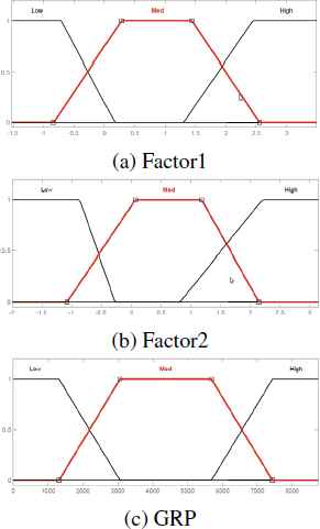
MFs of input variables for TOM prediction using all data.
5.3. ANN Architecture
In order to determine the structure of ANN and find the optimal parameters of NN, we applied training dataset to find the weights of hidden layer. Using these hidden layer weights, the minimum mean square error (MSE) between actual and ANN prediction are computed by validation dataset. Firstly, ANN method is applied to find MSE of TOM, SOV, and SA. Using all data, FMCG, and non-FMCG data, the minimum MSEs are presented in Tables A.1, A.2, and A.3, respectively (See Appendix A). To run the ANN model, different AF for output layer and hidden layer, learning rates, and numbers of hidden neurons are tried, and their corresponding MSEs are recorded. Ultimately, minimum MSEs specify the best architecture and the optimal parameters of ANN for each output variable.
The results of Tables A.1, A.2, and A.3 are summarized in Table 7.
| Data | Output | AF of Output Layer | AF of Hidden Layer | LR | # of Hidden Neurons |
|---|---|---|---|---|---|
| All | TOM | Tan-Sigmoid | Tan-Sigmoid | 0.7 | 10 |
| SOV | Tan-Sigmoid | Tan-Sigmoid | 0.6 | 12 | |
| SA | Tan-Sigmoid | Tan-Sigmoid | 0.6 | 10 | |
| FMCG | TOM | Tan-Sigmoid | Log-Sigmoid | 0.6 | 10 |
| SOV | Tan-Sigmoid | Tan-Sigmoid | 0.5 | 12 | |
| SA | Tan-Sigmoid | Log-Sigmoid | 0.6 | 12 | |
| Non-FMCG | TOM | Tan-Sigmoid | Tan-Sigmoid | 0.7 | 7 |
| SOV | Tan-Sigmoid | Tan-Sigmoid | 0.6 | 10 | |
| SA | Tan-Sigmoid | Tan-Sigmoid | 0.6 | 10 | |
The best ANN architecture using all, FMCG, and non-FMCG data.
5.4. ANFIS vs. ANN
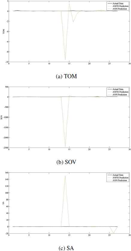
In order to compare ANFIS and ANN, a testing dataset should be used and the prediction results of the methods should be checked. As shown in Figures 7a, 7b, and 7c, actual data, ANFIS and ANN predictions of TOM, SOV, and SA are respectively depicted. According to Table 8, the correlation values of all data predictions, ANN provides better results than ANFIS in all the three metrics. These values also indicate that the predictions of TOM are more accurate than SOV and SA.
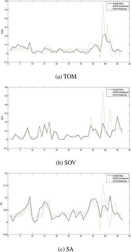
The actual, ANFIS, and ANN predictions of all data.
| Data | Output | ANFIS Correlation | ANN Correlation |
|---|---|---|---|
| All | TOM | 0.6520 | 0.8946 |
| SOV | 0.6287 | 0.8643 | |
| SA | 0.3762 | 0.8003 | |
| FMCG | TOM | 0.8701 | 0.9668 |
| SOV | 0.5327 | 0.9132 | |
| SA | 0.3132 | 0.7745 | |
| Non-FMCG | TOM | −0.0869 | 0.8189 |
| SOV | −0.3033 | 0.9551 | |
| SA | 0.2878 | 0.8426 | |
The correlations between actual data and predictions of ANFIS and ANN using all, FMCG, and non-FMCG data.
Using FMCG data, the graph of actual data, ANFIS and ANN predictions of TOM, SOV, and SA are displayed in Figures 8a, 8b, and 8c, respectively. As represented in Table 8, the correlations between actual and the predictions of ANN are much more than ANFIS predictions. Similar to all data predictions, TOM predictions has less errors and are more accurate than SOV and SA. As you can see in Figure 8b and 8c and the correlation values of FMCG predictions in Table 8, ANFIS provides very good prediction for TOM; however, the prediction of SOV and SA are not acceptable.
The actual, ANFIS, and ANN predictions of FMCG data.
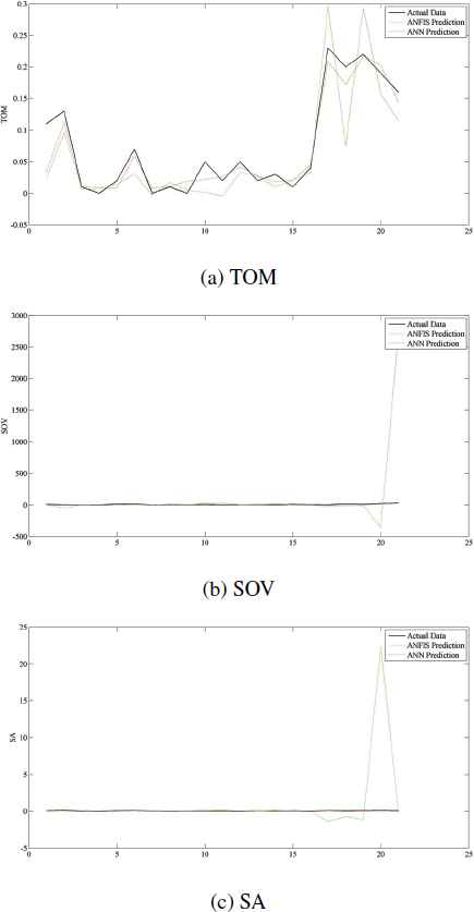
The prediction of ANFIS and ANN, and actual data of TOM, SOV, and SA using non-FMCG data are presented in Figures 9a, 9b, and 9c, respectively. The correlation values of ANFIS and ANN predictions reveal that ANN predictions and actual data are highly correlated, i.e. ANN provides better prediction than ANFIS. Unlike all and FMCG estimations, the predicted SOV using non-FMCG data represents better prediction of SOV, followed by SA and TOM.
The actual, ANFIS, and ANN predictions of non-FMCG data.
Due to lack of enough data of each company, we considered pooled data, namely all, FMCG, and non-FMCG to run ANFIS and ANN methods. However, we used each company’s data severally, and we found inaccurate prediction. So that each company’s prediction is not displayed here.
In order to compare the prediction ability of ANFIS and ANN by graphs, the testing dataset and the predicted values of ANFIS and ANN using all, FMCG and non-FMCG data are depicted in Figures 7, 8, and 9, respectively. In these figures, actual data, FMCG, and non-FMCG data are plotted by bold black, green dashed, and red dot dashed lines, respectively. To reach a fair comparison, we applied the most appropriate architecture of both ANFIS and ANN, and considered similar parameters for running ANFIS and ANN, i.e. the epochs and the percentage of testing data were the same in both methods.
As you can see in Figures 7, 8, and 9, in most of the cases, the red lines are closer to the bold black lines than the green lines, and in some cases green lines are detoured and become distant from the actual data. These outlier predictions of ANFIS also appeared in the structuring of ANFIS network in Section 5.2 (See Tables 3, 4, and 5). The reason of this detour cannot be clearly explained, but it can be related to the functioning of NN as a black box 23. These figures illustrate our previous findings regarding the superiority of ANN to ANFIS in predicting the brand image and advertising awareness data.
6. Conclusion
The proposed model applies adaptive neuro-fuzzy inference system and artificial neural network to evaluate the effect of brand image on advertising awareness. To investigate the advertising or brand awareness of 15 prominent Turkish brands, a field study was conducted and people were asked to respond a questionnaire. There were 30 questions whichformed the components of brand image and brand awareness, as well as three marketing metrics including TOM, SOV, and SA. Since running ANFIS and/or ANN with 30 variables is almost impossible, we used a dimension reduction method to reduce the number of input variables. Applying PCA for 30 given variables, two principle components are obtained. These two components plus GRP variable formed the input variables of ANFIS and ANN. And TOM, SOV, and SA are considered as the output variables of these methods.
To make the right prediction, given data is randomly split to three sets including training, validation, and testing datasets. The learning of training dataset leads to determining the weights of ANFIS and ANN and form the architecture of ANFIS and ANN, separately. Based on these networks, validation dataset will be applied and the least error between ANFIS and ANN predictions with actual data shows the optimal ANFIS and/or ANN structure. Finally, a testing dataset will be utilized to compare the prediction of ANFIS and ANN.
According to these correlations of actual data and predicted data, ANN provide more accurate predictions than ANFIS. Using all data, TOM data were perfectly correlated with the actual TOM values. The correlation of SOV and SA were smaller than TOM’s, but their predictions were highly correlated with the corresponding actual data as well. By analyzing the homogeneous companies and classifying them into FMCG and non-FMCG, the pooled data became consistent with each other, in some cases the errors of their predictions were less than all data. Using FMCG data, we estimated TOM, SOV, and SA separately. In both prediction methods, the correlations between given data and predictions revealed that TOM was the best predicted variable, followed by SOV and SA. In non-FMCG data, although ANN predictions and actual data are highly correlated, ANFIS presents weak predictions of all advertising awareness metrics. Among ANN predictions, SOV achieve the best prediction of output variables, followed by SA and TOM, respectively.
As future works, brand image components of other product categories such as durable goods or any other unknown data can be considered and prediction methods can be applied to estimate advertising awareness metrics. The prediction results can be investigated using other AI tools such as support vector machine, or recently developed deep learning methods like deep NN. Researchers can apply AI methods to other branches of management.
Appendix A
The minimum MSEs of ANN using all, FMCG, and non-FMCG data are presented in Tables A.1, A.2, and A.3, respectively.
| AF of Output Layer | AF of Hidden Layer | LR | # of Hidden Neurons | MSE of Training TOM | MSE of Validation TOM | MSE of Testing TOM | MSE of Training SOV | MSE of Validation SOV | MSE of Testing SOV | MSE of Training SA | MSE of Validation SA | MSE of Testing SA |
|---|---|---|---|---|---|---|---|---|---|---|---|---|
| Tan-Sigmoid | Tan-Sigmoid | 0.5 | 7 | 0.0010625 | 0.0003609 | 0.0008200 | 0.0005222 | 0.0002933 | 0.0002506 | 0.0003909 | 0.0004878 | 0.0002426 |
| Tan-Sigmoid | Tan-Sigmoid | 0.5 | 10 | 0.0012360 | 0.0004853 | 0.0010634 | 0.0004119 | 0.0000797 | 0.0010757 | 0.0003942 | 0.0001714 | 0.0004924 |
| Tan-Sigmoid | Tan-Sigmoid | 0.5 | 12 | 0.0026993 | 0.0031387 | 0.0037728 | 0.0005199 | 0.0013814 | 0.0001115 | 0.0003472 | 0.0004340 | 0.0001801 |
| Tan-Sigmoid | Tan-Sigmoid | 0.6 | 7 | 0.0010034 | 0.0007240 | 0.0008403 | 0.0007641 | 0.0001517 | 0.0003871 | 0.0003811 | 0.0001084 | 0.0002959 |
| Tan-Sigmoid | Tan-Sigmoid | 0.6 | 10 | 0.0009160 | 0.0004268 | 0.0034744 | 0.0004607 | 0.0001908 | 0.0011604 | 0.0002804 | 0.0001049 | 0.0005182 |
| Tan-Sigmoid | Tan-Sigmoid | 0.6 | 12 | 0.0009065 | 0.0009524 | 0.0018643 | 0.0011649 | 0.0000440 | 0.0017898 | 0.0003041 | 0.0004878 | 0.0002388 |
| Tan-Sigmoid | Tan-Sigmoid | 0.7 | 7 | 0.0012317 | 0.0008469 | 0.0015925 | 0.0006429 | 0.0028402 | 0.0004472 | 0.0003918 | 0.0003445 | 0.0003033 |
| Tan-Sigmoid | Tan-Sigmoid | 0.7 | 10 | 0.0010573 | 0.0000888 | 0.0007599 | 0.0011688 | 0.0001443 | 0.0001037 | 0.0003696 | 0.0008804 | 0.0005135 |
| Tan-Sigmoid | Tan-Sigmoid | 0.7 | 12 | 0.0011257 | 0.0013948 | 0.0008474 | 0.0005797 | 0.0002675 | 0.0004147 | 0.0007640 | 0.0004464 | 0.0004134 |
| Tan-Sigmoid | Log-Sigmoid | 0.5 | 7 | 0.0008774 | 0.0031034 | 0.0025585 | 0.0006460 | 0.0012700 | 0.0008111 | 0.0003294 | 0.0002133 | 0.0001197 |
| Tan-Sigmoid | Log-Sigmoid | 0.5 | 10 | 0.0010766 | 0.0006139 | 0.0013686 | 0.0007453 | 0.0003409 | 0.0003982 | 0.0004199 | 0.0003498 | 0.0002125 |
| Tan-Sigmoid | Log-Sigmoid | 0.5 | 12 | 0.0027888 | 0.0003046 | 0.0017654 | 0.0004002 | 0.0002354 | 0.0032802 | 0.0003364 | 0.0001076 | 0.0011938 |
| Tan-Sigmoid | Log-Sigmoid | 0.6 | 7 | 0.0009569 | 0.0014006 | 0.0020633 | 0.0005295 | 0.0000796 | 0.0009767 | 0.0003831 | 0.0001815 | 0.0002488 |
| Tan-Sigmoid | Log-Sigmoid | 0.6 | 10 | 0.0010707 | 0.0002682 | 0.0019027 | 0.0006799 | 0.0001001 | 0.0001710 | 0.0004079 | 0.0001346 | 0.0002792 |
| Tan-Sigmoid | Log-Sigmoid | 0.6 | 12 | 0.0012299 | 0.0015557 | 0.0006871 | 0.0006743 | 0.0002413 | 0.0009341 | 0.0003629 | 0.0003410 | 0.0003174 |
| Tan-Sigmoid | Log-Sigmoid | 0.7 | 7 | 0.0010207 | 0.0001581 | 0.0036420 | 0.0005780 | 0.0008884 | 0.0002994 | 0.0003148 | 0.0003112 | 0.0003271 |
| Tan-Sigmoid | Log-Sigmoid | 0.7 | 10 | 0.0009648 | 0.0007031 | 0.0010530 | 0.0004841 | 0.0001282 | 0.0007241 | 0.0005199 | 0.0002188 | 0.0002007 |
| Tan-Sigmoid | Log-Sigmoid | 0.7 | 12 | 0.0010871 | 0.0003526 | 0.0007603 | 0.0003846 | 0.0002811 | 0.0001653 | 0.0002635 | 0.0004140 | 0.0004899 |
| Log-Sigmoid | Tan-Sigmoid | 0.5 | 7 | 0.0068233 | 0.0098833 | 0.0085667 | 0.0180380 | 0.0191000 | 0.0128033 | 0.0007121 | 0.0003247 | 0.0007095 |
| Log-Sigmoid | Tan-Sigmoid | 0.5 | 10 | 0.0070642 | 0.0097747 | 0.0065887 | 0.0179103 | 0.0127568 | 0.0179437 | 0.0006973 | 0.0009265 | 0.0006837 |
| Log-Sigmoid | Tan-Sigmoid | 0.5 | 12 | 0.0069607 | 0.0080182 | 0.0082117 | 0.0178446 | 0.0181765 | 0.0157531 | 0.0007793 | 0.0011356 | 0.0005573 |
| Log-Sigmoid | Tan-Sigmoid | 0.6 | 7 | 0.0069343 | 0.0042317 | 0.0085686 | 0.0180500 | 0.0169158 | 0.0126144 | 0.0007199 | 0.0005490 | 0.0010413 |
| Log-Sigmoid | Tan-Sigmoid | 0.6 | 10 | 0.0070379 | 0.0026171 | 0.0063098 | 0.0178876 | 0.0158321 | 0.0166922 | 0.0007975 | 0.0004194 | 0.0002977 |
| Log-Sigmoid | Tan-Sigmoid | 0.6 | 12 | 0.0070491 | 0.0067731 | 0.0050644 | 0.0178807 | 0.0172284 | 0.0117882 | 0.0007510 | 0.0002008 | 0.0002725 |
| Log-Sigmoid | Tan-Sigmoid | 0.7 | 7 | 0.0070555 | 0.0093534 | 0.0074792 | 0.0178973 | 0.0168904 | 0.0171947 | 0.0007640 | 0.0009184 | 0.0011295 |
| Log-Sigmoid | Tan-Sigmoid | 0.7 | 10 | 0.0069180 | 0.0106027 | 0.0038627 | 0.0179483 | 0.0166403 | 0.0188720 | 0.0007391 | 0.0003411 | 0.0013955 |
| Log-Sigmoid | Tan-Sigmoid | 0.7 | 12 | 0.0070474 | 0.0059736 | 0.0077986 | 0.0177305 | 0.0176781 | 0.0189280 | 0.0007502 | 0.0007152 | 0.0004980 |
| Log-Sigmoid | Log-Sigmoid | 0.5 | 7 | 0.0072864 | 0.0078000 | 0.0043333 | 0.0178316 | 0.0168612 | 0.0195142 | 0.0007276 | 0.0005454 | 0.0006228 |
| Log-Sigmoid | Log-Sigmoid | 0.5 | 10 | 0.0072811 | 0.0068833 | 0.0055166 | 0.0182045 | 0.0134297 | 0.0162928 | 0.0007328 | 0.0004794 | 0.0003375 |
| Log-Sigmoid | Log-Sigmoid | 0.5 | 12 | 0.0072233 | 0.0067448 | 0.0085770 | 0.0182441 | 0.0141017 | 0.0136194 | 0.0006895 | 0.0007175 | 0.0007244 |
| Log-Sigmoid | Log-Sigmoid | 0.6 | 7 | 0.0072277 | 0.0085382 | 0.0065615 | 0.0180517 | 0.0179590 | 0.0123221 | 0.0006971 | 0.0006795 | 0.0015514 |
| Log-Sigmoid | Log-Sigmoid | 0.6 | 10 | 0.0072320 | 0.0064833 | 0.0084000 | 0.0180852 | 0.0171657 | 0.0185739 | 0.0006725 | 0.0013834 | 0.0009223 |
| Log-Sigmoid | Log-Sigmoid | 0.6 | 12 | 0.0070546 | 0.0074667 | 0.0050948 | 0.0180419 | 0.0146851 | 0.0232523 | 0.0007452 | 0.0009052 | 0.0010257 |
| Log-Sigmoid | Log-Sigmoid | 0.7 | 7 | 0.0070257 | 0.0084002 | 0.0060512 | 0.0181771 | 0.0122954 | 0.0188149 | 0.0007199 | 0.0007081 | 0.0006307 |
| Log-Sigmoid | Log-Sigmoid | 0.7 | 10 | 0.0072592 | 0.0052938 | 0.0082167 | 0.0178992 | 0.0190168 | 0.0260856 | 0.0007173 | 0.0003167 | 0.0009838 |
| Log-Sigmoid | Log-Sigmoid | 0.7 | 12 | 0.0070234 | 0.0082582 | 0.0058593 | 0.0179615 | 0.0250181 | 0.0169769 | 0.0007692 | 0.0007853 | 0.0008121 |
The MSE of training, validation and testing data sets and the architecture of ANN using all data.
| AF of Output Layer | AF of Hidden Layer | LR | # of Hidden Neurons | MSE of Training TOM | MSE of Validation TOM | MSE of Testing TOM | MSE of Training SOV | MSE of Validation SOV | MSE of Testing SOV | MSE of Training SA | MSE of Validation SA | MSE of Testing SA |
|---|---|---|---|---|---|---|---|---|---|---|---|---|
| Tan-Sigmoid | Tan-Sigmoid | 0.5 | 7 | 0.00052 | 0.00041 | 0.00261 | 0.00114 | 0.00058 | 0.00090 | 0.00040 | 0.00077 | 0.00060 |
| Tan-Sigmoid | Tan-Sigmoid | 0.5 | 10 | 0.00048 | 0.00004 | 0.00011 | 0.00076 | 0.00146 | 0.00018 | 0.00035 | 0.00008 | 0.00028 |
| Tan-Sigmoid | Tan-Sigmoid | 0.5 | 12 | 0.00058 | 0.00242 | 0.00297 | 0.00055 | 0.00003 | 0.00069 | 0.00024 | 0.00066 | 0.00183 |
| Tan-Sigmoid | Tan-Sigmoid | 0.6 | 7 | 0.00349 | 0.00031 | 0.00071 | 0.00067 | 0.00086 | 0.00013 | 0.00037 | 0.00009 | 0.00114 |
| Tan-Sigmoid | Tan-Sigmoid | 0.6 | 10 | 0.00091 | 0.00029 | 0.00021 | 0.00103 | 0.00014 | 0.00110 | 0.00054 | 0.00016 | 0.00050 |
| Tan-Sigmoid | Tan-Sigmoid | 0.6 | 12 | 0.00088 | 0.00120 | 0.00062 | 0.00059 | 0.00018 | 0.00057 | 0.00104 | 0.00042 | 0.00182 |
| Tan-Sigmoid | Tan-Sigmoid | 0.7 | 7 | 0.00063 | 0.00069 | 0.00047 | 0.00214 | 0.00369 | 0.00148 | 0.00035 | 0.00025 | 0.00095 |
| Tan-Sigmoid | Tan-Sigmoid | 0.7 | 10 | 0.00065 | 0.00137 | 0.00072 | 0.00075 | 0.00004 | 0.00020 | 0.00035 | 0.00011 | 0.00023 |
| Tan-Sigmoid | Tan-Sigmoid | 0.7 | 12 | 0.00065 | 0.00015 | 0.00424 | 0.00063 | 0.00019 | 0.00040 | 0.00044 | 0.00005 | 0.00026 |
| Tan-Sigmoid | Log-Sigmoid | 0.5 | 7 | 0.00094 | 0.00045 | 0.00182 | 0.00096 | 0.00060 | 0.00065 | 0.00052 | 0.00082 | 0.00064 |
| Tan-Sigmoid | Log-Sigmoid | 0.5 | 10 | 0.00120 | 0.00021 | 0.00267 | 0.00057 | 0.00005 | 0.00009 | 0.00048 | 0.00115 | 0.00076 |
| Tan-Sigmoid | Log-Sigmoid | 0.5 | 12 | 0.00071 | 0.00121 | 0.00172 | 0.00100 | 0.00063 | 0.00028 | 0.00032 | 0.00044 | 0.00107 |
| Tan-Sigmoid | Log-Sigmoid | 0.6 | 7 | 0.00410 | 0.00037 | 0.01274 | 0.00066 | 0.00010 | 0.00061 | 0.00045 | 0.00040 | 0.00036 |
| Tan-Sigmoid | Log-Sigmoid | 0.6 | 10 | 0.00050 | 0.00002 | 0.00003 | 0.00094 | 0.00008 | 0.00109 | 0.00036 | 0.00109 | 0.00068 |
| Tan-Sigmoid | Log-Sigmoid | 0.6 | 12 | 0.00060 | 0.00204 | 0.00274 | 0.00068 | 0.00004 | 0.00134 | 0.00030 | 0.00001 | 0.00012 |
| Tan-Sigmoid | Log-Sigmoid | 0.7 | 7 | 0.00102 | 0.00020 | 0.00279 | 0.00084 | 0.00104 | 0.00176 | 0.00086 | 0.00035 | 0.00081 |
| Tan-Sigmoid | Log-Sigmoid | 0.7 | 10 | 0.00089 | 0.00044 | 0.00011 | 0.00109 | 0.00060 | 0.00299 | 0.00047 | 0.00025 | 0.00011 |
| Tan-Sigmoid | Log-Sigmoid | 0.7 | 12 | 0.00072 | 0.00010 | 0.00006 | 0.00065 | 0.00026 | 0.00129 | 0.00041 | 0.00026 | 0.00056 |
| Log-Sigmoid | Tan-Sigmoid | 0.5 | 7 | 0.00741 | 0.00859 | 0.00702 | 0.01330 | 0.01504 | 0.01599 | 0.00063 | 0.00070 | 0.00080 |
| Log-Sigmoid | Tan-Sigmoid | 0.5 | 10 | 0.00738 | 0.00710 | 0.01007 | 0.01318 | 0.01423 | 0.02392 | 0.00079 | 0.00002 | 0.00088 |
| Log-Sigmoid | Tan-Sigmoid | 0.5 | 12 | 0.00744 | 0.01054 | 0.00911 | 0.01399 | 0.00996 | 0.02108 | 0.00070 | 0.00067 | 0.00060 |
| Log-Sigmoid | Tan-Sigmoid | 0.6 | 7 | 0.00729 | 0.01077 | 0.01077 | 0.01368 | 0.01297 | 0.01002 | 0.00080 | 0.00057 | 0.00127 |
| Log-Sigmoid | Tan-Sigmoid | 0.6 | 10 | 0.00747 | 0.00430 | 0.00820 | 0.01361 | 0.01557 | 0.00229 | 0.00091 | 0.00014 | 0.00087 |
| Log-Sigmoid | Tan-Sigmoid | 0.6 | 12 | 0.00755 | 0.00737 | 0.00395 | 0.01324 | 0.01362 | 0.02000 | 0.00069 | 0.00054 | 0.00115 |
| Log-Sigmoid | Tan-Sigmoid | 0.7 | 7 | 0.00762 | 0.00937 | 0.00754 | 0.01342 | 0.00935 | 0.01584 | 0.00075 | 0.00041 | 0.00041 |
| Log-Sigmoid | Tan-Sigmoid | 0.7 | 10 | 0.00741 | 0.01080 | 0.01077 | 0.01379 | 0.01724 | 0.01453 | 0.00106 | 0.00030 | 0.00065 |
| Log-Sigmoid | Tan-Sigmoid | 0.7 | 12 | 0.00752 | 0.00623 | 0.00687 | 0.01326 | 0.01573 | 0.01691 | 0.00073 | 0.00116 | 0.00049 |
| Log-Sigmoid | Log-Sigmoid | 0.5 | 7 | 0.00783 | 0.00394 | 0.00683 | 0.01357 | 0.01100 | 0.01152 | 0.00071 | 0.00037 | 0.00099 |
| Log-Sigmoid | Log-Sigmoid | 0.5 | 10 | 0.00760 | 0.00960 | 0.00807 | 0.01424 | 0.00928 | 0.01162 | 0.00078 | 0.00050 | 0.00084 |
| Log-Sigmoid | Log-Sigmoid | 0.5 | 12 | 0.00805 | 0.00989 | 0.00963 | 0.01324 | 0.01389 | 0.01985 | 0.00077 | 0.00172 | 0.00105 |
| Log-Sigmoid | Log-Sigmoid | 0.6 | 7 | 0.00735 | 0.01057 | 0.00843 | 0.01399 | 0.02073 | 0.01168 | 0.00075 | 0.00072 | 0.00049 |
| Log-Sigmoid | Log-Sigmoid | 0.6 | 10 | 0.00752 | 0.00493 | 0.00840 | 0.01399 | 0.01001 | 0.02253 | 0.00066 | 0.00029 | 0.00043 |
| Log-Sigmoid | Log-Sigmoid | 0.6 | 12 | 0.00807 | 0.00511 | 0.01364 | 0.01357 | 0.01206 | 0.00820 | 0.00070 | 0.00093 | 0.00119 |
| Log-Sigmoid | Log-Sigmoid | 0.7 | 7 | 0.00768 | 0.00970 | 0.00540 | 0.01421 | 0.00602 | 0.01635 | 0.00072 | 0.00052 | 0.00154 |
| Log-Sigmoid | Log-Sigmoid | 0.7 | 10 | 0.00800 | 0.00817 | 0.01363 | 0.01389 | 0.01780 | 0.01941 | 0.00084 | 0.00031 | 0.00073 |
| Log-Sigmoid | Log-Sigmoid | 0.7 | 12 | 0.00785 | 0.00833 | 0.00739 | 0.01360 | 0.00720 | 0.01046 | 0.00074 | 0.00093 | 0.00022 |
The MSE of training, validation and testing data sets and the architecture of ANN using FMCG data.
| AF of Output Layer | AF of Hidden Layer | LR | # of Hidden Neurons | MSE of Training TOM | MSE of Validation TOM | MSE of Testing TOM | MSE of Training SOV | MSE of Validation SOV | MSE of Testing SOV | MSE of Training SA | MSE of Validation SA | MSE of Testing SA |
|---|---|---|---|---|---|---|---|---|---|---|---|---|
| Tan-Sigmoid | Tan-Sigmoid | 0.5 | 7 | 0.0006319 | 0.0003101 | 0.0025939 | 0.0001299 | 0.0000577 | 0.0000088 | 0.0002376 | 0.0001172 | 0.0019135 |
| Tan-Sigmoid | Tan-Sigmoid | 0.5 | 10 | 0.0007877 | 0.0001980 | 0.0022569 | 0.0001115 | 0.0002863 | 0.0000218 | 0.0003505 | 0.0000295 | 0.0004397 |
| Tan-Sigmoid | Tan-Sigmoid | 0.5 | 12 | 0.0010455 | 0.0003094 | 0.0015051 | 0.0000952 | 0.0000022 | 0.0011033 | 0.0002507 | 0.0000129 | 0.0004678 |
| Tan-Sigmoid | Tan-Sigmoid | 0.6 | 7 | 0.0007381 | 0.0003452 | 0.0050689 | 0.0002436 | 0.0000272 | 0.0000210 | 0.0002590 | 0.0000520 | 0.0000361 |
| Tan-Sigmoid | Tan-Sigmoid | 0.6 | 10 | 0.0010991 | 0.0001751 | 0.0014006 | 0.0000819 | 0.0000001 | 0.0000124 | 0.0003684 | 0.0000060 | 0.0005198 |
| Tan-Sigmoid | Tan-Sigmoid | 0.6 | 12 | 0.0013379 | 0.0001534 | 0.0032945 | 0.0002327 | 0.0000091 | 0.0001148 | 0.0001970 | 0.0000605 | 0.0004542 |
| Tan-Sigmoid | Tan-Sigmoid | 0.7 | 7 | 0.0009631 | 0.0000557 | 0.0061017 | 0.0001800 | 0.0004179 | 0.0000610 | 0.0005921 | 0.0000128 | 0.0000561 |
| Tan-Sigmoid | Tan-Sigmoid | 0.7 | 10 | 0.0011145 | 0.0030957 | 0.0004129 | 0.0000885 | 0.0000038 | 0.0001801 | 0.0004065 | 0.0001027 | 0.0006073 |
| Tan-Sigmoid | Tan-Sigmoid | 0.7 | 12 | 0.0007791 | 0.0002126 | 0.0015490 | 0.0002777 | 0.0000822 | 0.0002778 | 0.0003031 | 0.0000985 | 0.0000399 |
| Tan-Sigmoid | Log-Sigmoid | 0.5 | 7 | 0.0020955 | 0.0002610 | 0.0002825 | 0.0001700 | 0.0001387 | 0.0000030 | 0.0003328 | 0.0000251 | 0.0004266 |
| Tan-Sigmoid | Log-Sigmoid | 0.5 | 10 | 0.0008679 | 0.0001704 | 0.0045356 | 0.0001231 | 0.0000370 | 0.0010916 | 0.0011866 | 0.0000222 | 0.0004996 |
| Tan-Sigmoid | Log-Sigmoid | 0.5 | 12 | 0.0007269 | 0.0003237 | 0.0006901 | 0.0001258 | 0.0000329 | 0.0010424 | 0.0002354 | 0.0000264 | 0.0004451 |
| Tan-Sigmoid | Log-Sigmoid | 0.6 | 7 | 0.0007939 | 0.0000826 | 0.0004704 | 0.0001508 | 0.0000291 | 0.0003674 | 0.0003393 | 0.0001446 | 0.0002840 |
| Tan-Sigmoid | Log-Sigmoid | 0.6 | 10 | 0.0010658 | 0.0001791 | 0.0009399 | 0.0002813 | 0.0000301 | 0.0001140 | 0.0002759 | 0.0002106 | 0.0004508 |
| Tan-Sigmoid | Log-Sigmoid | 0.6 | 12 | 0.0009880 | 0.0006585 | 0.0002235 | 0.0002589 | 0.0000229 | 0.0005966 | 0.0006831 | 0.0005519 | 0.0002748 |
| Tan-Sigmoid | Log-Sigmoid | 0.7 | 7 | 0.0007908 | 0.0006926 | 0.0002700 | 0.0001983 | 0.0001071 | 0.0000192 | 0.0002365 | 0.0000953 | 0.0000105 |
| Tan-Sigmoid | Log-Sigmoid | 0.7 | 10 | 0.0007153 | 0.0011456 | 0.0025772 | 0.0001203 | 0.0000018 | 0.0002070 | 0.0002979 | 0.0005045 | 0.0000200 |
| Tan-Sigmoid | Log-Sigmoid | 0.7 | 12 | 0.0015587 | 0.0000839 | 0.0006243 | 0.0007323 | 0.0003332 | 0.0004638 | 0.0002860 | 0.0000984 | 0.0001085 |
| Log-Sigmoid | Tan-Sigmoid | 0.5 | 7 | 0.0039610 | 0.0064667 | 0.0051747 | 0.0110311 | 0.0167383 | 0.0119643 | 0.0005874 | 0.0009189 | 0.0006103 |
| Log-Sigmoid | Tan-Sigmoid | 0.5 | 10 | 0.0040370 | 0.0033080 | 0.0042297 | 0.0113621 | 0.0124732 | 0.0077596 | 0.0006112 | 0.0009212 | 0.0012659 |
| Log-Sigmoid | Tan-Sigmoid | 0.5 | 12 | 0.0039984 | 0.0059333 | 0.0035587 | 0.0114564 | 0.0098871 | 0.0022256 | 0.0006005 | 0.0008338 | 0.0010649 |
| Log-Sigmoid | Tan-Sigmoid | 0.6 | 7 | 0.0039550 | 0.0059667 | 0.0060000 | 0.0111753 | 0.0060603 | 0.0137983 | 0.0005598 | 0.0016583 | 0.0006703 |
| Log-Sigmoid | Tan-Sigmoid | 0.6 | 10 | 0.0040982 | 0.0016667 | 0.0025667 | 0.0112098 | 0.0143126 | 0.0046021 | 0.0005888 | 0.0012183 | 0.0003877 |
| Log-Sigmoid | Tan-Sigmoid | 0.6 | 12 | 0.0040428 | 0.0018593 | 0.0053667 | 0.0114813 | 0.0113233 | 0.0085511 | 0.0006361 | 0.0004709 | 0.0005943 |
| Log-Sigmoid | Tan-Sigmoid | 0.7 | 7 | 0.0039919 | 0.0077520 | 0.0020897 | 0.0112945 | 0.0082144 | 0.0064858 | 0.0005961 | 0.0007586 | 0.0003367 |
| Log-Sigmoid | Tan-Sigmoid | 0.7 | 10 | 0.0040181 | 0.0048667 | 0.0036920 | 0.0112655 | 0.0106808 | 0.0119597 | 0.0006011 | 0.0008648 | 0.0007766 |
| Log-Sigmoid | Tan-Sigmoid | 0.7 | 12 | 0.0040088 | 0.0033000 | 0.0057630 | 0.0110717 | 0.0167674 | 0.0101679 | 0.0005981 | 0.0003622 | 0.0010030 |
| Log-Sigmoid | Log-Sigmoid | 0.5 | 7 | 0.0040582 | 0.0053667 | 0.0010297 | 0.0112291 | 0.0096340 | 0.0177958 | 0.0006481 | 0.0001510 | 0.0001307 |
| Log-Sigmoid | Log-Sigmoid | 0.5 | 10 | 0.0039894 | 0.0041000 | 0.0060127 | 0.0112547 | 0.0125351 | 0.0135128 | 0.0005740 | 0.0014169 | 0.0017704 |
| Log-Sigmoid | Log-Sigmoid | 0.5 | 12 | 0.0040519 | 0.0056630 | 0.0010734 | 0.0111838 | 0.0174942 | 0.0123807 | 0.0006370 | 0.0009676 | 0.0007749 |
| Log-Sigmoid | Log-Sigmoid | 0.6 | 7 | 0.0039140 | 0.0082831 | 0.0059001 | 0.0112513 | 0.0114197 | 0.0148093 | 0.0006303 | 0.0007222 | 0.0013911 |
| Log-Sigmoid | Log-Sigmoid | 0.6 | 10 | 0.0039952 | 0.0045334 | 0.0052667 | 0.0112433 | 0.0129049 | 0.0137578 | 0.0006572 | 0.0004843 | 0.0001689 |
| Log-Sigmoid | Log-Sigmoid | 0.6 | 12 | 0.0040374 | 0.0025667 | 0.0049500 | 0.0113340 | 0.0140143 | 0.0077465 | 0.0006369 | 0.0011818 | 0.0005853 |
| Log-Sigmoid | Log-Sigmoid | 0.7 | 7 | 0.0040563 | 0.0028333 | 0.0036667 | 0.0112107 | 0.0119741 | 0.0164474 | 0.0005718 | 0.0005763 | 0.0009703 |
| Log-Sigmoid | Log-Sigmoid | 0.7 | 10 | 0.0040001 | 0.0036333 | 0.0059000 | 0.0112383 | 0.0161540 | 0.0107778 | 0.0006799 | 0.0000258 | 0.0009023 |
| Log-Sigmoid | Log-Sigmoid | 0.7 | 12 | 0.0040405 | 0.0055497 | 0.0018000 | 0.0111559 | 0.0144121 | 0.0169658 | 0.0006419 | 0.0001896 | 0.0012903 |
The MSE of training, validation and testing data sets and the architecture of ANN using non-FMCG data.
References
Cite this article
TY  - JOUR
AU  - Ali Fahmi
AU  - Kemal Burc Ulengin
AU  - Cengiz Kahraman
PY  - 2017
DA  - 2017/02/09
TI  - Analysis of Brand Image Effect on Advertising Awareness Using A Neuro-Fuzzy and A Neural Network Prediction Models
JO  - International Journal of Computational Intelligence Systems
SP  - 690
EP  - 710
VL  - 10
IS  - 1
SN  - 1875-6883
UR  - https://doi.org/10.2991/ijcis.2017.10.1.46
DO  - 10.2991/ijcis.2017.10.1.46
ID  - Fahmi2017
ER  -