
A Logical Deduction Based Clause Learning Algorithm for Boolean Satisfiability Problems
- DOI
- 10.2991/ijcis.2017.10.1.55How to use a DOI?
- Keywords
- Boolean Satisfiability; SAT Problem; Clause Learning; Logical Deduction; Implication Graph
- Abstract
Clause learning is the key component of modern SAT solvers, while conflict analysis based on the implication graph is the mainstream technology to generate the learnt clauses. Whenever a clause in the clause database is falsified by the current variable assignments, the SAT solver will try to analyze the reason by using different cuts (i.e., the Unique Implication Points) on the implication graph. Those schemes reflect only the conflict on the current search subspace, does not reflect the inherent conflict directly involved in the rest space. In this paper, we propose a new advanced clause learning algorithm based on the conflict analysis and the logical deduction, which reconstructs a linear logical deduction by analyzing the relationship of different decision variables between the backjumping level and the current decision level. The logical deduction result is then added into the clause database as a newly learnt clause. The resulting implementation in Minisat improves the state-of-the-art performance in SAT solving.
- Copyright
- © 2017, the Authors. Published by Atlantis Press.
- Open Access
- This is an open access article under the CC BY-NC license (http://creativecommons.org/licences/by-nc/4.0/).
1. Introduction
Boolean satisfiability (SAT) problem is the first NP-complete problem proven by Cook2, many problems can be converted into the SAT problem solving. The corresponding SAT solvers are widely used in combinatorial optimization, artificial intelligence, model checking, integrated circuit verification, software verification, and other fields. Over the last two decades, many heuristic algorithms for SAT solvers have been developed, such as clause learning3,4,15, non-chronological backtracking4, branching heuristic4,6,19,20, restart5,21,22, clause deleting6,23, and so on. With the help of those algorithms, the modern SAT solvers can solve the problem with millions of clauses, and those algorithms also enhance the chances for the SAT solvers to be widely applied in industry.
Among the key technologies of SAT solvers, clause learning is the most important one. In the search procedure, whenever a new decision variable is chosen, the Boolean Constraint Propagation algorithm (BCP) can determine the values of a series of variables. If any clause in the clause database is falsified, the conflict analysis procedure will be triggered, and new learnt clauses are obtained by analyzing the implication graph and added into the original problem3. The learnt clauses often make other clauses become redundant, i.e., the learnt clauses can simplify the original problem, but also avoid the solver enter the same conflict search space again. Implication graph and other advanced researches on learning clauses, such as efficient implementation7, minimizing learnt clauses7, measuring the quality of learnt clause and subgraph8,10, extending implication graph9, and so on, have made a great breakthrough in the performance of the SAT solver.
However, the implication graph processing usually does not consider the relationship between different decision variables, but focuses on how to cut the implication graph and obtain the corresponding learnt clauses. Because the literals involved in the learnt clause cannot be assigned false at the same time, implication subgraph reflects only conflicts caused by the assigned variables, therefore it cannot fully reflects the potential conflicts in the rest graph. In Ref. 11, Jabbour used learnt clause and original clause for resolution deduction, and the resolvent was added to the clause database as the new learnt clause and obtained a smaller backjumping level at the same time. The new learnt clause is not directly related to the current conflict. Although the potential conflicts seem to be processed, but sometimes it is hard to pinpoint the deep reasons of the conflict. In Ref. 29, Sabharwal used the implication graph to generate additional clauses called back-clauses. By adding the first Unique Implication Point (UIP) clause and back-clauses between every two consecutive UIPs at level L, it enable unit propagation to make all inferences that all traditional nogoods based on all UIPs at level L would. This method only analyzes the reason of conflict at the single decision level, and does not consider the relationship between the different decision levels, so the effect of corresponding back-clause is not obvious.
Aiming to find the relationship between different decision variables, and avoid the potential conflicts, we use logical deductive method with a systematic study of the conflict analysis and clause learning in this paper. Whenever a conflict is reached, the solver begins to reconstruct a logical deduction by using decision variables between the backjumping level and the current decision level, and the results is then added to the original problem for further search. Experiments show that the proposed algorithm has significantly improved the frequency of restarts, conflicts and decision-making. The rest of the paper is organized as follows. Section 2 provides some preliminaries including the main concepts used in the present work. Section 3 summarizes some traditional learning schemes. Then a new approach using logical deduction for clause learning is proposed and detailed in Section 4. It is followed by the experimental case studies and results analysis in Section 5. Section 6 concludes the paper.
2. Preliminaries
2.1. SAT problem
A propositional formula ϕ is represented in a Conjunctive Normal Form (CNF) which consists of a conjunction of clauses C, ϕ is true if and only if all of its clauses are true. A clause C consists of a disjunction of literals l, C is true while one of its literals is true. A literal l is either a variable x or its negation –x, i.e., if x is assigned value true (1), then –x must be false (0), and vice versa. For example, ϕ0 = (–x1 ˅ x3) ˄ (x1 ˅ x2) ˄ (x2 ˅ –x3 ˅ x5) ˄ (–x2 ˅ –x4 ˅ –x5) is a CNF formula which contains 5 variables and 4 clauses.
The SAT problem is to decide whether there exists a truth assignment to all the variables such that the formula ϕ becomes true. If exist, then ϕ is satisfiable; otherwise ϕ is unsatisfiable. For the formula ϕ0, the assignment X’ = {x1 = 1, x2 = 1, x3 = 1, x4 = 0} makes it true, so ϕ0 is satisfiable, we call X′ is a satisfiable instance or interpretation of ϕ0.
2.2. CDCL framework
Conflict-Driven Clause Learning (CDCL) is based on the Davis–Putnam–Logemann–Loveland (DPLL)12,13 algorithm, which is the most mainstream architecture of the modern SAT solver. Typical CDCL SAT solver algorithm24 is shown in Algorithm 1. The SAT solver records an index for each decision level, which is denoted as decisionlevel, the decisionlevel starts from 0. Each variable in a CNF formula has a unique decision level, denoted as Lx. The search procedure will start by selecting an unassigned variable p and assume a value for it, at the same time, a new decision level will be starting, while the decisionlevel adds 1 by itself and the search space will jump to v ∪{p}. BCP(ϕ, v) is the Boolean Constraint Propagation (BCP) procedure that consists of the iterated application of the unit clause rule. During these running procedures, a sequence of literals will be derived from it, and we call such variables propagated variables, denoted as V |p, and Lp = L V|p. Let Root(x) be a function defined as the decision level which variable x belongs to, then Root(p) = p, Root(V |p) = p. If a conflict occurs in BCP(ϕ, v), i.e., any clause, either the initial clause or learnt clause, becomes an empty clause, then the procedure will analyze the reason of conflict, obtain a learnt clause and a backjumping decision level β. If β is 0, representing that the conflict occurs at the top level, then ϕ is unsatisfiable; otherwise undo all assignments between β and the current decision level.
| Input: CNF formula ϕ, assigned variables v. | |
| Output: the property of ϕ. | |
| 1: | decisionlevel ← 0 |
| 2: | if (BCP (ϕ, v)==CONFLICT) then ⪧ Boolean Constraint Propagation |
| 3: | return UNSATISFIABLE |
| 4: | while (not AllVariableAssigned(ϕ, v)) |
| 5: | p ← PickBranchingLit (ϕ, v) ⪧ Start a new branch |
| 6: | decisionlevel ← decisionlevel +1 |
| 7: | v ← v∪{p} |
| 8: | if (BCP (ϕ, v)==CONFLICT) then |
| 9: | β = ConflictAnalysis(ϕ, v) |
| 10: | if(β < 0) then ⪧ Conflict occurred at the root level |
| 11: | return UNSATISFIABLE |
| 12: | else |
| 13: | BackTrack(ϕ, v, β) ⪧ Non-chronological backtracking |
| 14: | decisionlevel ← β |
| 15: | return SATISFIABLE |
A typical CDCL framework.
3. Clause learning
In the subsequent sections we will review the clause learning method, resolution and implication graph, and how to analyze the conflict and obtain the learnt clause from an implication graph.
3.1. Resolution
Resolution principle14,16 is one of the most important methods for validating the unsatisfiability of logical formulae. Given two clauses C1 = A ˅ x and C2 = B ˅ –x, where x is a Boolean variable, then the clause R(C1, C2) = A ˅ B can be inferred by the resolution rule, resolving on the variable x. R(C1, C2) is called the resolvent of C1 and C2, both C1 and C2 is either a clause of original formula or the resolvent iteratively derived by using the resolution rule. If R(C1, C2) is an empty clause, then the original formula is unsatisfiable. The resolvent can be viewed as a learnt clause puts into the CNF formula, but it is not directly derived from the conflict. In theory, the number of resolvents from a CNF formula is infinite, often requires amazing time and space complexity.
3.2. Implication Graph
CDCL based on implication graph3 makes the scale of learnt clauses obvious smaller than the conventional resolution, and more targeted. The main idea of this method is as follows: whenever the conflict occurs, i.e., there exists at least one clause whose literals are all false, then analyze the implication graph and find the reason of conflict, and a new learnt clause represents the conflict is derived and added to the CNF formula.
The implication graph reflects the relationships of assigned variables during the SAT solver process. An implication graph is a directed acyclic graph (DAG). A typical implication graph is illustrated in Fig. 1, which is constructed as follows:
- •
Vertex: each vertex represents a variable assignment and its decision level, e.g., in Fig. 1, x1(6) represents the variable x1 is assigned true at the decision level 6, –x8(6) represents the variable x8 is assigned false at the decision level 6.
- •
Directed edge: the directed edge propagates from the antecedent vertices to the vertex q corresponding to the unit clause Ci that led to q assigned true, which will be labeled with Ci. Vertices have no incident edges corresponding to the decision variables. In Fig. 1, x4 and x1 are assigned false at the decision level 3 and 6, respectively, so C1 is a unit clause at the moment, its sole unassigned literal x3 must be assigned true for C1 to be satisfied. Therefore, –x4(3) and –x1(6) are the antecedent vertices of x3(6).
- •
Conflict: each variable corresponds to a unique vertex in the implication graph. A conflict occurs when there is a variable appears with positive and negative at the same time, such variable is referred to as the conflicting variable. In Fig. 1, x2 is the conflicting variable. In this case, the search procedure will be broken and the conflict analysis procedure will be invoked.
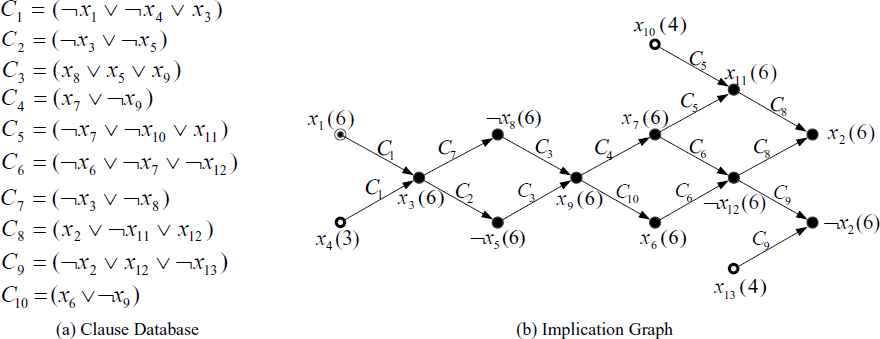
Clause database and implication graph.
Unique Implication Point3: A Unique Implication Point (UIP) is a vertex in an implication graph that dominates both positive and negative branches of the conflicting variable. In Fig. 1, x9 has played a dominant role for the conflict branches x2 and –x2. Therefore, x9 is a UIP. From the conflicting variable, along the incident edge backtrack to the current decision variable, UIPs are sorted in order as follows: called x9 the First UIP, x3 is the Last UIP.
3.3. Conflict Analysis and Learning
Conflict analysis aims to find the reasons of conflict, such conflict is not always caused by a unique variable assignment. As shown in Fig. 1, in addition to the variable x1 assigned true at the current decision level, x4, x10 and x13 are assigned true at the earlier decision level. Through the conflict analysis, we can construct a new clause C′ = (–x1 ˅ –x4 ˅ –x10 ˅ –x13) as a constraint clause and put it into the initial clause database, and backtrack to the biggest level except the current conflict level, see Ref. 15. Whenever the variables x4, x10 and x13 are assigned true, x1 must be assigned false for C′ to be satisfied, i.e., the SAT solver will not enter the conflict search space again.
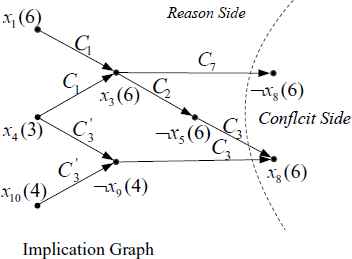
When the conflict occurs, different learnt clauses can be deduced from the implication graph by different UIP cuts. The implication graph will be divided into two parts, that is, the conflict side and the reason side. The conflict side contains the conflict variables, and the reason side contains the variable which caused the conflict. Grasp3 and Chaff4 used the First UIP cut, as shown in Fig. 2, the first UIP splits the implication graph by the unique implication point x9, the corresponding learnt clause (–x9 ˅ –x10 ˅ –x13) will be derived. Relsat15 used the Last UIP cut schema, the corresponding learnt clause is (–x1 ˅ –x4 ˅ –x10 ˅ –x13), and backtrack to level 4.

Different cuts on an implication graph.
In Ref. 9, Audemard proposed an extension of the clause learning method called inverse arcs, which is directly derived from the satisfied clause. As shown in Fig. 1, for the clause C1 = (–x1 ˅ –x4 ˅ x3), x1 is assigned true at the current decision level, x4 is assigned true at the smaller decision level, such that x3 will be assigned true at the current decision level, both x1 and x4 are the antecedent variables of x3. Assume that there exists a clause C′ = (x4 ˅ –x14 ˅ –x3), x3 is assigned true at the level 2, the literal x4 assigned at the level 7 is implied by the two literals x14 and x3 respectively assigned at the levels 2 and 6. So the clause C’ is an inverse arc, the new clause R(C′,CLastUIP) = (–x1 ˅ –x10 ˅ –x13 ˅ –x14 ˅ –x3) is generated by resolution, then the search procedure will backtrack to the level 2, which is smaller than the previous value, i.e., the conflict can be found as early as possible.
From the above analysis, CFirstUIP, CLastUIP and R(C′, CLastUIP) are different cuts and processes based on the current implication graph, the learnt clause is a constraint condition with part of a few variables. Although the inverse arc can derive a smaller backtracking level, but it usually requires amazing amount of calculation. The motivation behind the present work is to seek an advanced learning algorithm, making the backtracking level smaller, amounts of calculation fewer, and the optimization efficiency higher. In order to break through the limit of classical learning schemes, we have done some research on logical deduction, see Ref. 1, another automated reasoning method. Experiments show that the combination of implication graph and logical deduction is effective for some hard distances. Accordingly, in this paper, we propose an advanced learning algorithm based on the logical deduction. Through the analysis of correlation information between the decision variables at different decision levels, the proposed learning algorithm constructs the information constraints out of the implication graph, so as to guide the search process to avoid conflict as early as possible. The new learning algorithm is detailed in the following Section 4.
4. An Advanced Clause Learning Algorithm Using Logical Deduction
4.1. Principle
In this section, we propose a new approach using logical deduction for clause learning, and the logical method we used is mainly base on the resolution principle and its variations. Due to its simplicity, as well as its soundness and completeness, resolution method has been adopted by the most popular modern theorem provers. For further improving the efficiency of resolution, many refined resolution methods have been proposed such as linear resolution, semantic resolution, and lock resolution, etc. In this paper we use the structure of linear resolution deduction as the logical deduction method, in which many clauses are involved in the deduction, only one resolvent is derived.
Definition 4.116,25
Let C1 and C2 be clauses and L1 a propositional variable. Then the clause R(C1,C2,Li) = C′1 ˅ C′2 is called a resolvent of clauses C1 = (L1 ˅ C′1) and C2 = (–L1 ˅ C′2).
Definition 4.225
Let S be a clause set. ω = {C1, C2, …, Ck} is called a resolution deduction from S to Ck, if Ci (i = 1,…, k) is either a clause in S, or the resolvent of Cj. and Cr (j < i, r < i).
Definition 4.325
Let S be a clause set, C0 a clause in S. Then ω = {C1, C2, …, Ck} is called a linear resolution deduction from S to Ck with the top clause C0 (shown in Fig. 3).
- (1)
Ci+1 is the resolvent of Ci (a center clause) and Bi (a side clause), where i = 0, 1, …, k–1;
- (2)
Bi ∈ S, or Bi = Cj.(j < i).
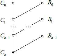
Classical linear resolution.
4.2. Extension
As shown in Fig. 3, the resolution process is pushed forward from top to bottom with top clause C0, any Ci (1 ≤ i ≤ k) can be viewed as a learnt clause. Observe that the classical linear resolution is merely theoretical, and there have three uncertain factors (or defects) that limit the computer implementation:
- (1)
Uncertain Resolution Literal. Each resolution literal li belongs to Ci, any literal in Ci can be selected as a resolution literal li. Different li may generates the different resolvent Ci+1.
- (2)
Uncertain Side Clause. Whenever a center clause Ci and its resolution literal li are determined, any clause (including original clause and resolvent) which contains –li can be selected as side clause, so the arbitrariness of choosing side clause is increased sharply while generating new resolvents.
- (3)
Uncertain Depth. Here, the depth is k which represents the number of center clauses. If the last center clause Ck is nonempty and resolution literal is not pure literal, then the resolution deduction will be extended sustainably. Therefore, k is uncertain.
In general, for a large-scale CNF formula, the resolvents are often grown exponentially with the depth of the solution. Therefore, in a logical deduction, which clause should be chosen and how many literals are involved, will make a lot of influences on the efficiency of solving. In response to these uncertain factors, we present some extended strategies of integrating with CDCL solver. The logical deduction process can be invoked at any time of the CDCL search procedure, restrictive strategies make the resolving process more controllable and easily realized.
(1) Synchronized Clause Learning (SCL). Linear logical deduction process synchronized with the CDCL clause learning. After the CDCL conflict analysis, a backtracking level is obtained, then we can reconstruct a linear resolution deduction between the backtracking level (also the root level) and the current decision level. Decision variables from the backtracking level to the current decision level are sequentially selected as the resolution literal. Our motivation is to prevent the resolution literals are arbitrarily selected. Further, the depth of resolution deduction is determined by backtracked level. Restrictive resolution literals and depth make the resolving process is controllable.
As an example illustrated in Fig. 4, assume that Fig. 4(a) is a partial sequence of variable assignments under the current conflict, where decision variables are grayed out and other variables behind the decision variable are implied variables under the corresponding decision assignments. When the conflict occurred at the current decision level 10, the backtracking level is 7 according to the CDCL conflict analysis, then our algorithm is invoked. Decision variables from the backtracking level to the current decision level are x3, x11, x5 and x16 respectively. With those decision variables, we can reconstruct a logical resolution deduction and get a new clause completely different from the procedure via the implication graph. The reconstructed process is shown in Fig. 4(b), where C′0, B′0, B′1, B′2 is part of C0, B0, B1, B2, respectively. The resolvent C3 = (x16 ˅ C′0 ˅ B′0 ˅ B′1 ˅ B′2) can be added to the clause database as a new learnt clause. Moreover, we can reconstruct another logical deduction shown in Fig. 4(c). Notice that the center clause C0 and the side clauses B0, B1, and B2 are different from that shown in Fig. 4(b). Here, we add a tautology B3 = (x16 ˅ –x16) to the clause database. Then the resolvent C4 = (–x16 ˅ C′0 ˅ B′0 ˅ B′1 ˅ B′2) is also a learnt clause, which contains the negation of the last decision variable x16 and similar to the traditional learnt clause by cutting the implication graph.
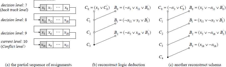
The partial sequence of assignments under the current conflict and the reconstruct logical deduction by using those decision variables.
(2) Smaller Average Decision Level (SADL). For the side clause Bi, the average decision level excluding the unassigned literals should be as small as possible, and the number of unassigned literals must be as less as possible. There are two advantages for those selection strategies: one is the side clauses can be easily determined rather than randomly chosen, and therefore it can be seen as the conflict variables guided. The other and the most important is that, the smaller average decision level will cause the backtracking level smaller, i.e., the conflicts will occur as earlier as possible. On the other hand, the clauses with less unassigned literals are more likely unsatisfied, i.e., it is easier to become a unit clause or binary clause, hence it reduce the searching space more powerful.
(3) Periodical Resolvent Deletion (PRD). In most cases the resolvents are grown exponentially, we need to construct automatic garbage collection that prevents memory overflow. It means, in short, the resolvents should be deleted periodically. However, it is not easy to estimate which one is best resolvent among those. In Ref. 17, Minisat set an activity weight for each learnt clause. Whenever a learnt clause takes part in the conflict analysis, its activity is bumped. Inactive clauses are periodically removed. In Refs. 23 and 26, Glucose compute the Literals Blocks Distance (LBD) for each learnt clause. A learnt clause is partitioned into n subsets according to the decision level of its literals, then all the learnt clauses with LBD greater than 2 are periodically deleted. Inspired by Minisat and Glucose, we propose a new weighted activity evaluation for each resolvent as follows:
Definition 4.4 (Weighted Activity -WA).
Let S be a clause set and ω = {C1, C2,…,Ck} be a linear resolution deduction from S to Ck with the top clause C0. The number of resolvent Ci that takes part in the conflict analysis is defined as H(Ci). The average decision level of resolvent Ci is defined as L(Ci). We define the weighted activity of Ci as
The new advanced algorithm is shown in Algorithm 2, Through many times deductions by recursively selected clause Bi, the resolvent Ci+1 can be added to the original CNF formula, which will not change the truth-value of the formula.
| Input: backtracking level backlevel after conflict analysis. | |
| Output: a new learnt clause by a logical deduction. | |
| 1: | while (backlevel < decisionlevel) ⪧ decisionlevel : the current decision level. |
| 2: | i ← 0 |
| 3: | p = trail[Lastbacklevel] ⪧ trail: the sequence of assigned variables. |
| 4: | q = trail[Lastbacklevel +1] |
| 5: | Bi =getClause(–p, q) ⪧ Choose a clause which contains both –p and q. |
| 6: | if (Bi is existing) |
| 7: | C′i+1 = R(C′i, Bi) ⪧ Use the resolution rule on p with C′i and Bi. |
| 8: | else |
| 9: | break ⪧ Stop deduction. |
| 10: | i ← i +1 |
| 11: | backlevel ← backlevel +1 |
| 12: | return C′i+1 |
The advanced clause learning by using the logical deduction.
4.3. Compare with First UIP Cut
Let’s recall the example shown in Fig. 2, where the current decision level is 6. After a conflict occurs, a new learnt clause CLastUIP = (¬x1 ˅ ¬x4 ˅ ¬x10 ˅ ¬x13) can be inferred from the implication graph by the Last UIP cut. Because Lx4 < Lx10 ≤ Lx13 < Lx1, the search procedure will get back to the second largest decision level 4. In this case, we can choose the smallest decision level Lx4 = 3. We start the logical deduction from the layer 3 to 6 (also starts from the root level). Assume that Root(¬x4) = x14 and Root(¬x10) = x15, the decision variable of level 5 is x16, there exist clauses C11 = (¬x4 ˅ x14), C12 = (x15 ˅ ¬x14 ˅ ¬x9), C13 = (¬x15 ˅ x16 ˅ ¬x10), and C14 = (¬x16 ˅ ¬x9), we can infer some clauses by the logical deduction:
The clause database and implication graph based on the logical deduction.
5. Experimental Results
In this section, we empirically compare the performance between the SAT solvers with and without using the logical deduction. Minisat17 is the well-known SAT solver with the First UIP, some state of the art SAT solvers such as Glucose, abcdSAT and COMiniSatPS are improved versions on the Minisat, see Refs. 26–28. So we have implemented the logical deduction with different backlevel in Minisat 2.2.0, called PSat_bl0 and PSat_blc respectively with the backlevel 0 and the backlevel from the conflict analysis. This comparison is made on the set of 286 instances from the main track of SAT-Race 2015, with a time out of 3600s. We used a farm of Xeon 2.4Ghz E5 with 16G bytes physical memory, the operating system is Hat Enterprise Red 6.
Both Minisat 2.2.0 and PSat can successfully solve the instances without any preprocessors and all conclusions are correct. Minisat 2.2.0 solved 170 instances, PSat with backlevel=0 solved 193 instances, and PSat with backlevel from the conflict analysis solved 203 instances. For the satisfiable problems, PSat_blc solves 20 more instances than Minisat. For the unsatisfiable problems, PSat_blc solves 13 more instances than Minisat. Table 1 summarizes the number of instances solved for different benchmark families, where some families have been cleared from the table that all solvers have equal numbers of solved instances.
| Family | Minisat 2.2.0 | PSat_bl0 | PSat_blc | ||||||
|---|---|---|---|---|---|---|---|---|---|
|
|
|||||||||
| SAT | UNSAT | TOTAL | SAT | UNSAT | TOTAL | SAT | UNSAT | TOTAL | |
| manthey | 36 | 28 | 64 | 37 | 29 | 66 | 41 | 29 | 70 |
| jgiraldezlevy | 13 | 0 | 13 | 14 | 0 | 14 | 16 | 1 | 17 |
| xbits | 12 | 0 | 12 | 17 | 0 | 17 | 17 | 0 | 17 |
| atco | 4 | 4 | 8 | 4 | 5 | 9 | 6 | 5 | 11 |
| 6sx | 0 | 2 | 2 | 0 | 3 | 3 | 0 | 4 | 4 |
| aaaix-planning | 0 | 0 | 0 | 0 | 2 | 2 | 0 | 2 | 2 |
| ACG | 0 | 1 | 1 | 1 | 2 | 3 | 1 | 2 | 3 |
| aes | 2 | 0 | 2 | 1 | 0 | 1 | 4 | 0 | 4 |
| AProVE | 1 | 0 | 1 | 1 | 2 | 3 | 1 | 2 | 3 |
| Group_mulr | 0 | 0 | 0 | 0 | 1 | 1 | 0 | 1 | 1 |
| gss | 2 | 0 | 2 | 2 | 0 | 2 | 3 | 0 | 3 |
| mrpp | 20 | 12 | 32 | 21 | 12 | 33 | 20 | 12 | 32 |
| partial | 3 | 0 | 3 | 3 | 0 | 3 | 2 | 0 | 2 |
| UCG | 2 | 1 | 3 | 3 | 2 | 5 | 3 | 2 | 5 |
| UR | 0 | 0 | 0 | 1 | 0 | 1 | 1 | 0 | 1 |
| UTI | 0 | 0 | 0 | 1 | 0 | 1 | 1 | 0 | 1 |
| countbitssr | 0 | 0 | 0 | 0 | 1 | 1 | 0 | 1 | 1 |
| vmpc | 2 | 0 | 2 | 2 | 0 | 2 | 1 | 0 | 1 |
Zoom on some solved families.
The manthey family18 is encoding of the Modulo game, a certain form of a combinatorial puzzle. We can see that our approach improves most obviously on the manthey family.
Table 2 shows the average time of Minisat, PSat_bl0 and PSat_blc. As can be seen clearly, the logical deduction with the advanced clause learning method performs better than the original version no matter on SAT or UNSAT instances. For the satisfiable problems, Minisat solved 114 instances with average time 715.6s, but PSat_blc requires only 305.8s for 134 instances. This illustrates the learnt clauses from reconstructing logical deduction are more efficient because of avoiding the potential conflict searching space. For the unsatisfiable problems, PSat_blc solved 69 instances with average time 958.9s. It seems that the time is long compared to the result in Minisat and PSat_bl0. The reason is PSat_blc solved more difficult instances which are spent nearly 3600s. Fig. 6 shows that both PSat_bl0 and PSat_blc are more powerful than Minisat, where each dot corresponds to a SAT instance. Although the two versions of the PSat can improve the efficiency significantly, they behave differently, backlevel from conflict analysis is better than directly selecting the top level. The reason is that the logical deduction tends to spend more time, sometimes the learnt clauses have more literals while more clauses participates in the logical deduction and become redundant easily.
| Solver | Minisat 2.2.0 | PSat_bl0 | PSat_blc | ||||||
|---|---|---|---|---|---|---|---|---|---|
|
|
|||||||||
| SAT | UNSAT | TOTAL | SAT | UNSAT | TOTAL | SAT | UNSAT | TOTAL | |
| Solved instances | 114 | 56 | 170 | 126 | 67 | 193 | 134 | 69 | 203 |
| Total time(s) | 81578 | 35629 | 117207 | 84372 | 42036 | 126408 | 40982 | 66164 | 107146 |
| Average time(s) | 715.6 | 636.2 | 689.5 | 669.6 | 627.4 | 655.0 | 305.8 | 958.9 | 527.8 |
The average time of different solvers.
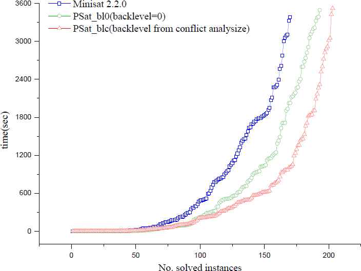
Cactus plot of solvers with different clause learning schemas (2015 SAT-Race instances).

Comparison of conflict times with and without the advanced learning on 156 instances.
6. Conclusions
In this paper, we have proposed an advanced learning algorithm for SAT problem. Whenever the SAT solver reaches a conflict, the advanced learning procedure will be triggered. A backjumping level is obtained by analyzing the implication graph. Through the iteratively logical deduction from the backjumping level to the current conflict level, a new learnt clause is obtained. The classic learning algorithms usually make the conflict occurs as early as possible, but easy to fall into a local optimum. As an extension of classic algorithms, our learnt clause contains more literals with smaller decision level, i.e. the possibility of SAT solver back- jump to the lower level will be bigger than before. We integrated the new algorithm into the state-of-the-art CDCL solver Minisat 2.2.0, experiments on the main track instances from SAT-Race 2015 showed that our algorithm has better performance. In future work, we plan to establish a detailed characterization system of clauses, in order to estimate clause of logical deduction, and obtain shorter resolvents.
Acknowledgements
This work is partially supported by the National Natural Science Foundation of China (Grant No. 61673320, 11526171, 61305074), and the Fundamental Research Funds for the Central Universities of China (Grant No. A0920502051305-24, 2682015CX060).
References
Cite this article
TY  - JOUR
AU  - Qingshan Chen
AU  - Yang Xu
AU  - Jun Liu
AU  - Xingxing He
PY  - 2017
DA  - 2017/04/03
TI  - A Logical Deduction Based Clause Learning Algorithm for Boolean Satisfiability Problems
JO  - International Journal of Computational Intelligence Systems
SP  - 824
EP  - 834
VL  - 10
IS  - 1
SN  - 1875-6883
UR  - https://doi.org/10.2991/ijcis.2017.10.1.55
DO  - 10.2991/ijcis.2017.10.1.55
ID  - Chen2017
ER  -