
Modeling Users’ Data Traces in Multi-Resident Ambient Assisted Living Environments
- DOI
- 10.2991/ijcis.10.1.88How to use a DOI?
- Keywords
- Ambient assisted living (AAL); smart environments; conditional least squares (CLS) estimation; aggregate data; Markov chain; multi-resident environments
- Abstract
Modeling users’ data traces is of crucial importance for human behavior analysis and context-aware applications in ambient assisted living (AAL) environments. However, learning the parameters of the underlying model is a challenging task in multi-occupant environments; because, the anonymous users’ data traces are aggregated temporally. This paper proposes a novel method for modeling users’ data traces in multi-resident sensor-based AAL environments. A Markov chain was considered as the underlying model. We aimed at estimating the parameters of the Markov chain directly out of users’ aggregate data. For this purpose, we hired the idea of conditional least squares (CLS) estimation. However, the CLS estimations can be inconsistent in the circumstances of AAL environments. To tackle this problem, we proposed to regularize the CLS estimations using spatial information of sensors. This information was extracted using an accessibility graph, made out of the deployed sensor network. To evaluate the proposed method, a well-known and publicly available dataset was used. The proposed method was compared with the standard CLS, using Kullback-Leibler (KL) divergence, and mean squared error (MSE) criteria. The results conveyed that the proposed method results in estimations with lower KL divergences from ground truth, compared to CLS. Also, the proposed method outperformed CLS with a MSE of 2.7 × 10⁻³.
- Copyright
- © 2017, the Authors. Published by Atlantis Press.
- Open Access
- This is an open access article under the CC BY-NC license (http://creativecommons.org/licences/by-nc/4.0/).
1. Introduction
The general goal of AAL is to hire ambient intelligence (AmI) and pervasive computing solutions to assist individuals with specific needs. To achieve this goal, the users’ data are captured by various types of sensors in the environment.1 The data is then analyzed using human behavioral models to predict or recognize the inhabitants’ upcoming actions. This, in turn, allows to provide necessary services for the residents. In order to preserve noninvasive and privacy-friendly characteristics of AAL environments, many researchers opt simple environmental binary sensors.2 We considered such sensors in the present work, too.
The analysis of inhabitants’ behaviors is the cornerstone of developing context-aware applications in an AAL environment.2–8 This can be performed by modeling traces of users’ sensory data. Residents’ behaviors, and in turn, their traces can be effectively modeled by Markov models (MMs).2,5,9–12 Although learning the parameters of such models is a straightforward task in single user environments, it is a challenging issue in multi-occupant environments. Because, in a multi-occupant environment, the traces are interwoven temporally; hence, a dataset of separated users’ traces is not available beforehand for training or designing a model. In this case, the sensors’ data is called aggregate data.13,14Conditional least squares (CLS) 13,14 is a method of estimating the parameters of a Markov model out of aggregate data. However, its performance would degenerate due to being inconsistent in the circumstances of AAL environments.
The main contribution of this paper is to address the problem of modeling users’ data traces in multi-occupant AAL environments. For this purpose, an ergodic, time-homogeneous, and stationary Markov chain was considered as the underlying model. We aimed at the problem of estimating parameters of the Markov chain directly out of aggregated users’ data. It was assumed that individuals behave independently according to the same Markov chain, and at each time step, an observation, was made out of the activated sensors’ data. The idea of CLS was incorporated to estimate the parameters of Markov chain. However, since CLS can be inconsistent in AAL environments, we proposed to regularize its estimations. This task was performed using the relation between spatial characteristics of sensors and their transition probabilities. The sensors’ spatial information was obtained by constructing an accessibility graph out of the deployed sensor network. This information was plugged into the optimization problem of CLS as a regularization term. It resulted in a novel convex optimization problem, whose solution yielded the ultimate estimations.
The remainder of the paper is organized as follows. In section 2, the related works are reviewed; network settings, and environmental states are discussed in section 3; the characteristics of users’ data traces, and problem statement are addressed in section 4; the standard CLS estimation is detailed in section 5; section 6 elaborates the proposed method; the experiments and results are taken in section 7; and finally, section 8 concludes the paper.
2. Related Works
Modeling users’ data traces is of crucial importance for context-aware applications in AAL environments. Some related applications include the approaches of Refs. 3, 6, 15, 16. In Ref. 3, a security surveillance system is designed to safeguard a building against intruders. In this system, the security guards are dispatched to the possible locations of intruders by predicting their trajectories. The modeling of users’ traces is performed by clustering possible traces. In Ref. 16, the mobility traces of a resident are modeled by flow graphs in an AAL environment. The extracted model is used to recognize the salient movement patterns which pertain to human activities that last for a while. In Ref. 15, a trajectory propagation algorithm is proposed to generate the possible sensor data traces, starting from the current state of the resident. For this purpose, the traces are assumed to be generated according to a spatial bipartite graph model, which is made according to the concurrent activations of sensors. In Ref. 6, a distributed abnormal activity detection approach, called DetectingAct, is proposed. In DetectingAct, an activity is defined as the combination of traces of sensor activations and their durations, and an abnormal activity is defined as the one which deviates from the normal routines. The abnormality of an activity is determined by comparing it with the normal patterns, using a number of similarity measures. Some other applications of modeling users’ data traces include user localization,4 health-care,7 and analyzing the performance of working places.8
Probabilistic graphical models have proven to be effective in modeling users’ behaviors, and users’ data traces in AAL environments.17 Thus far, Markov chains and hidden Markov models (HMMs),9,10,18 conditional random fields (CRFs),19 Bayesian networks,20 and their several variants have been adapted for human behavior modeling. These schemes are based on the Markov assumption that: the next step of a user’s activity depends on a limited history of the previous steps and sensors’ observations. Accordingly, the data traces can also be modeled based on this assumption. The works of Refs. 2, 5, 11, 12 are instances of such approaches. In Ref. 2, a framework, named FindingHumo, is proposed to extract the traces of multiple users for the purpose of multi-subject tracking in an AAL environment. In this work, a variable state and variable order HMM is constructed for fixed length time windows of sensor activations. The set of activated sensors in a time window together with their neighboring sensors compose the states of HMM in that window. The most likely users’ traces are obtained in each time window by Viterbi decoding algorithm. In this work, the transition probabilities of HMMs are obtained using either a training set of previously extracted trajectories, or some prior knowledge on the network topology. In Ref. 5, the sensor data traces of multiple users are extracted using Markov models for human behavior analysis. In this work, each sensor event is attributed to a user’s identifier (ID) by computing the most likely resident’s ID, given all of the sensor events up to the current time. In this work, a Markov model is trained for each resident. The transition probabilities are calculated based on a training set. In Refs. 11, 12, a system is proposed for data collection in indoor smart environments to lower the congestion and the communication cost between the sensors and the base station. These methods are based on the prediction of sensors’ data according to the knowledge, mined from users’ data traces. In this work, the model of the traces is considered to be a Markov chain.
In many applications of AAL environments, including the above-mentioned approaches, the model of the users’ data traces are obtained by manually and meticulously analyzing the preexistent data. This becomes a cumbersome and error-prone process, especially when coping with multi-resident AAL environments, in which the users’ traces are temporally aggregated, and the volume of data can drastically increase.
3. Network Settings and Environmental States
We considered a typical network of environmental binary sensors which is common in smart home environments. They can be categorized into two types according to their role: motion sensors, and item sensors. Motion sensors reveal the movement of the residents, while item sensors disclose the interactions of users with specific objects.
The value of sensors along time can reflect the state of the environment. To calculate the environmental states, the time-line was discretized into evenly separated time spans, namely Δt. Timespan Δt was selected such small that an activated sensor in each time span could be assumed to be triggered by a single user. The state of the environment was calculated in each time span as described in definition 1.
Definition 1.
(environmental states). Having n sensors, a vector xt ∈ {0,1}n is calculated for each time span t, whose i’ th element xt,i shows the value of sensor i at this time span. xt is named the environmental state at time t.
Figure 1 shows an example of users’ sensory data and the associated sequence of environmental states. In this example, there are three sensors and two users in the AAL environment. The sensory data is also shown on a timing diagram. As it is shown in the due table, users’ data are interwoven along time. Therefore, users’ data is called aggregate data. In fact, this aggregate data is composed of multiple traces of users’ data. These traces are shown in Fig. 2 and discussed in the next section. We aim at modeling these constituent traces in the following sections.
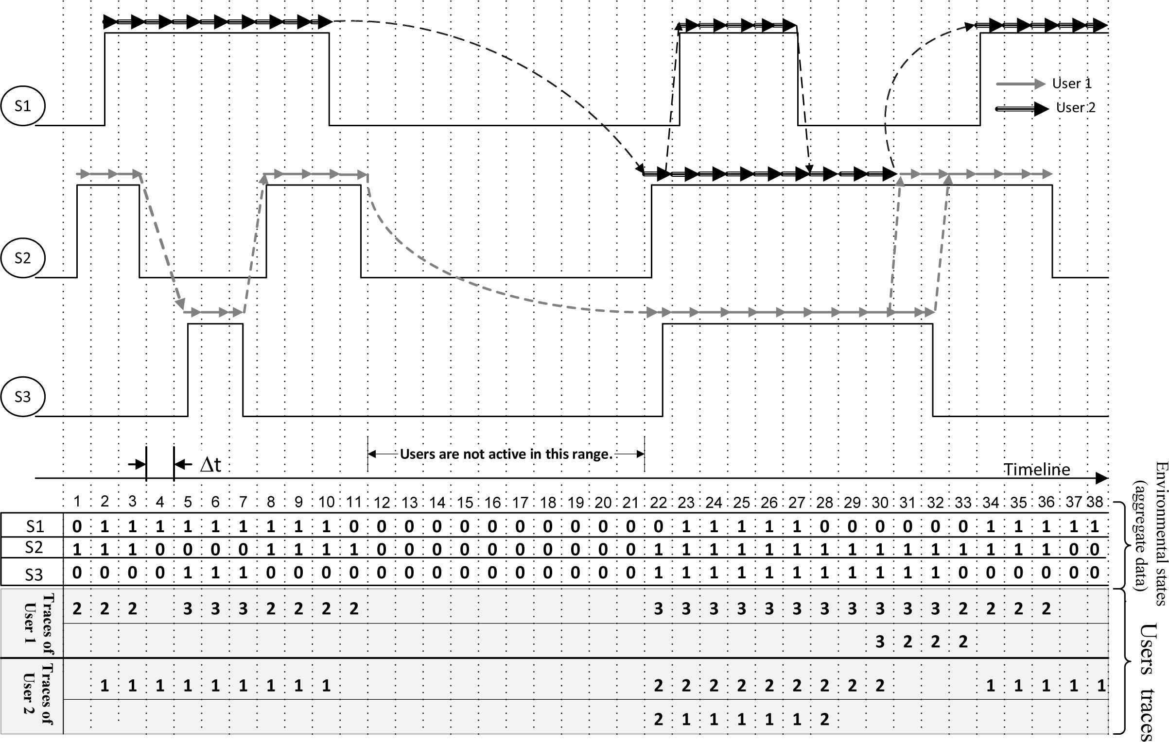
Sensory users’ data and the associated environmental states (aggregate data). Users’ data traces along time. The users’ traces are marked by arrows on the timing diagram, and also shown in the shaded Gant chart along time.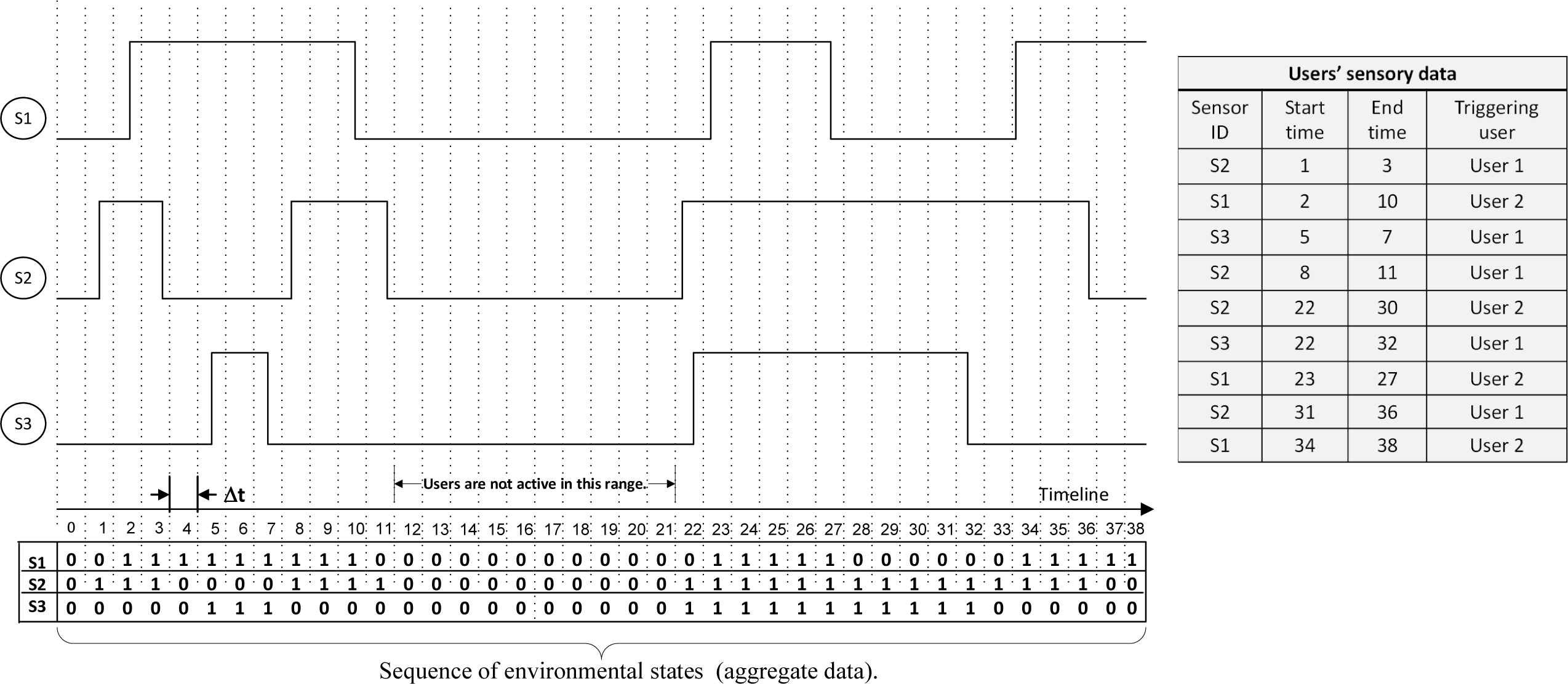
4. Users’ Traces and Problem Statement
A user’s data trace is a sequence of activated sensors in consecutive time slices, triggered by the same user. An example of data traces is taken in Fig. 2. It conforms to the aggregate sensory data of Fig. 1. Each user has generated two data traces. For instance, as it is shown, user 1 has generated traces: i) 2,2,2,3,3,3,2,2,2,2,3,3,3,3,3,3,3,3,3,3,3,2,2,2,2, and ii) 3,2,2,2. Generating more than a single trace by the same user is due to the fact that a user can trigger more than one sensor at the same time. The aggregation of these traces along time makes up the entire users’ sensory data of Fig. 1. We aimed at modeling these traces.
The users’ behaviors, and in turn users’ traces, can be effectively modeled by Markov models in AAL environments.5,9,10 We considered an ergodic, time-homogeneous, and stationary Markov chain on the state space S = {1,…,n}, where i ∈ S denotes the sensor ID, and n is the total number of sensors. Since this Markov model is stationary, its parameters do not depend on time. It was also considered that the initial state probabilities equal the stationary distribution. Therefore, the probability of a trace, denoted by R = r1,r2,…,rT,ri ∈ S, is calculated as:
Since the chains are started with the stationary distribution, the only parameters to estimate, are the transition probabilities in matrix P. Parameter estimation becomes a straight forward task, if the traces have been already extracted. In this case, the maximum likelihood estimation (MLE) is:
Although the use of MLE is straightforward, it needs previously extracted traces for the purpose of training. This becomes an error-prone and cumbersome task in realistic multi-user AAL environments, since a huge amount of data could have been aggregated. Therefore, we did not plan to extract the traces out of sensors’ data beforehand. In other words, the transition matrix should be estimated directly out of aggregate data. This problem is defined as in definition 2.
Definition 2.
(problem statement). Given a sequence of environmental states (i.e. aggregate data) in an AAL environment, estimate the transition matrix of an ergodic, time-homogeneous, and stationary Markov chain, i.e. matrix P, that can generate the constituent traces in the aggregate data.
In continue, the idea of conditional least squares estimation is discussed as a primitive solution for this problem.
5. Conditional Least Squares
Conditional least squares (CLS) 14 is a traditional method for estimating the transition matrix of a Markov chain out of aggregate data. According to the main idea of CLS, it is expected that for a sequence of the environmental states of length T, environmental state xt should be close to its conditional expectation, given xt−1. This can be termed formally as:
With regard to Eq. 4, the transition matrix P can be estimated by minimizing a least squares system as in Eq. 5.
It is well known that PCLS is asymptotically consistent when T → ∞ (i.e. plimT→∞PCLS = P).13,14 However, there are two drawbacks in CLS estimation: i) it can be proven that CLS is not consistent when the aggregate data is noisy (which is the case in AAL environments),13 and ii) the asymptotic condition of infinite sequence of environmental states, i.e. T → ∞, may not be satisfied in practice. Therefore, the estimated PCLS will diverge from ground truth values, empirically.
6. Proposed Method to Estimate the Markov Chain Parameters
In this section, we first introduce accessibility graphs along with an assumption to address the relation between spatial information of sensors and their transition probabilities. Then, based on this assumption, a regularization process is explained to mitigate the inconsistency effects of CLS.
6.1. Accessibility graphs and the proposed assumption
Given a sensor network with the characteristics mentioned in section 3, a graph can be made out of it. This is called the accessibility graph and is defined as in definition 3.
Definition 3.
(accessibility graph). Let S = {1,,n} denote the set of installed sensor IDs in a network of motion and item sensors. The undirected graph G = (V,E), with the set of vertices V and the set of edges E, is called the accessibility graph of the sensor network, if:
- •
V=S, and
- •
For sensors i, j ∈ S, the edge ei,j = (i, j) belongs to E, if sensor j can be directly triggered (accessed) after sensor i without triggering other sensors.
An example of the accessibility graph is shown in Fig. 3. This graph can be obtained by considering the sensing ranges of motion sensors i.e. sensors’ labels started by ”M”, and situations of item sensors.
The accessibility graph for the sensor network of a smart home (owing to the smart home map, designed in Ref. 18). The boxes and ovals show the sensors, and the links between them show the edges of the graph. Sensing ranges of sensors ”M023” and ”M022” are shaded.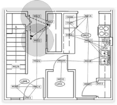
Intuitively, when a resident walks or interacts with objects in the AAL environment, it is expected that the sensors close to each other, should be triggered consecutively. This intuition is also discussed in Ref. 21. Therefore, it is inspired that: the more close two sensors are in the accessibility graph, the higher probability of being consecutive in a trace they will have.
Let G = (V,E) denote an accessibility graph, i, j ∈ V denote two vertices, and D(i, j) show the distance between i and j in the accessibility graph, such that it equals the minimum number of edges from i to j in G. Also, let P(i, j) denote the transition probability from sensor i to sensor j. According to the above-mentioned discussion, we made an assumption as defined in the following definition.
Definition 4.
(proposed assumption). The lower the spatial distance D(i, j) is, the higher the value of P(i, j) will be.
It should be noted that the increase or decrease of P(i, j) can be linear or non-linear in the distance between sensors i and j. We considered a linear rate, proportional to the exponent of the distances between sensors.
It is worth mentioning that one can integrate further spatial information by changing the definition of neighborhoods in the accessibility graph. For instance, one may observe that sensors installed in the same room are likely to be triggered consecutively. To include this contextual information, the vertices pertaining to sensors installed in the same room are considered as neighbors. In this case, a complete sub-graph is constructed by adding sufficient edges between the due vertices in the accessibility graph.
6.2. Regularizing the CLS estimations
As discussed earlier, we planned to regularize CLS estimations to mitigate the effect of noise and finite aggregate data. This task was performed according to the assumption, made in definition 4. This assumption was termed formally, and plugged into the optimization problem of CLS, i.e. Eq. 6, as a regularization term. This process resulted in a novel convex optimization problem as:
In the convex optimization problem of Eq. 7, the term
The solution of the convex optimization problem of Eq. 7 yields the final regularized estimated transition matrix, i.e. Pproposed.
Summing it up together, to model traces in a multi-resident AAL environment, an ergodic, time-homogeneous, and stationary Markov chain is considered. With this model, the only parameter to estimate, is the due transition matrix. For this purpose, firstly the accessibility graph is obtained for the underlying sensor network according to definition 3, and the distance matrix D is calculated accordingly. Secondly, having a dataset of sequences of environmental states (i.e. aggregate data), which has been collected in the environment, matrices of current and next environmental states, i.e. binary matrices X and Y, are calculated as described in Eq. 6. At last, the convex minimization problem of Eq. 7 is solved to yield the estimated transition matrix. Parameter lambda in Eq. 7 should be determined empirically by analyzing a small portion of the dataset.
7. Experiments and Results
In this section, the performance of the proposed method is compared with that of CLS. Each row of a transition matrix shows an independent posterior distribution, given a sensor event. That is, the elements of row i make up the probability distribution of the next sensor activation, given that sensor i is currently activated. Accordingly, to measure the efficiency of an estimation method, the row-wise Kullback-Leibler (KL) divergence of the estimated transition matrix from the ground truth transition matrix was calculated.
Let PG denote the ground truth transition matrix. Then, the row-wise KL divergence from an estimated transition matrix, namely
We also calculated the entry-wise mean squared errors (MSEs) of the estimated matrices. For an estimated transition matrix
The ground truth transition matrix, i.e. PG, is considered as the transition matrix of a Markov chain which can best generate the data traces of individuals in the dataset. Given a dataset of separated users’ traces, one can hire maximum likelihood estimation (MLE) to calculate this transition matrix. This is exactly the same as training a typical Markov chain on a dataset of sequences. However, in our research, the data traces of users are aggregated in the dataset, i.e. the traces of two or more users are interwoven and they are not clearly separated beforehand. Therefore, we first precisely extracted individual traces of users out of aggregate data manually, and then applied MLE on the set of extracted traces to learn the ground truth transition matrix. Extraction of users’ traces was performed using the IDs of users who triggered the sensors. These labels were available in the dataset. The ground truth transition matrix was only used for assessing the performance of the proposed method.
7.1. The dataset
A well-known and publicly available multi-resident smart home dataset, named Kyoto,18 from the Center for Advanced Studies in Adaptive Systems (CASAS) smart house project*, was used in the simulations. This dataset represents the sensor events pertaining to 20 pairs of participants performing their daily activities in an apartment. For each sensor event, its date, time, sensor ID, sensor value, and the ID of the resident who triggered it, is available. This dataset well suits our experiments; because, the generated sensory data are fully labeled by residents’ IDs in order to extract individual data traces, and in turn, to compute the ground truth transition matrix effectively.
7.2. Experimental settings
There are some parameters that should be determined in the experiments. One parameter is Δt, that was set to half a second, i.e. 50 milliseconds. The other parameter is the regularization coefficient λ in Eq. 7. A small portion of the dataset was used as the training set (around 5% of the consecutive sensor events) to determine this parameter. We extracted the users’ traces manually out of this small training set, and estimated a transition matrix using MLE, named Ptrain. Afterwards, a grid search strategy was conducted to determine λ. That is, Pproposed was calculated via Eq. 7 on the training set with various values of λ. The value that minimized the total row-wise KL divergence from Pproposed to Ptrain, was selected for λ. The total row-wise KL divergence (TRWKLD) was calculated as in Eq. 10. Accordingly, we set λ = 0.05 in our experiments.
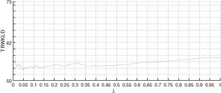
The grid search results to determine parameter λ. λ = 0.05 yields the minimum TRWKLD.
7.3. Implementation results
To assess the performance, we first conducted a paired t-Test and also calculated Pearson correlations to measure the difference between estimated and ground truth transition matrices. The paired t-test was performed at a significance level of α = 0.05. The null hypothesis H0 : µd = 0 was tested against H1 : µd ≠ 0, where µd denotes the mean of element-wise differences between an estimated transition matrix (i.e. either PCLC or PProposed) and the ground truth transition matrix. The results are depicted in Table 1. As it can be seen, the resulting P-values are higher than α, which means that no significant difference between estimated and ground truth transition matrices can be concluded. Also, the Pearson correlation between the estimated and ground truth transition probabilities has been more than 0.7. This testifies a strong linear relationship between estimated and ground truth values. In addition, the results showed that the elements of transition matrix estimated by the proposed method have a higher correlation (around 79.9%) with the ground truth values, compared to CLS. In continue, CLS and the proposed method are compared via KL divergence and MSE too.
| Parameter | CLS | PM |
|---|---|---|
| α | 0.05 | 0.05 |
| Number of observations | 1156 | 1156 |
| Pearson Correlation | 0.743 | 0.799 |
| Hypothesized Mean Difference | 0 | 0 |
| t-Stat | 0.026 | 0.071 |
| P-value one-tail | 0.489 | 0.472 |
| P-value two-tail | 0.979 | 0.944 |
PM=Proposed Method
Paired t-Test results and Pearson correlations.
As discussed earlier, the i’th row in a transition matrix shows the posterior distribution of sensor activations, given that sensor i is currently activated. We compared the proposed method with CLS in term of the row-wise KL divergence of their resulting transition matrices from the ground truth, according to Eq. 8. The results are depicted in Fig. 5. In this figure, the KL divergence of estimated posterior distributions, given each sensor, from the ground truth is calculated. As it can be seen, given an arbitrary sensor, the proposed method has resulted in a lower or comparable KL divergence, compared to CLS. This testifies that incorporating the spatial information of sensors has been effective in estimating the parameters of Markov chain, i.e. the transition matrix.
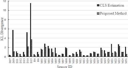
The KL divergence from the estimated posterior distributions to the ground truth posterior distributions, given a currently activated sensor.
For further assessments, we also calculated the entry-wise MSEs of the transition matrices PCLS, and Pproposed via Eq. 9. The results showed that Pproposed, and PCLS have MSEs of 2.7 × 10⁻³ and 3.2× 10⁻³, respectively. Therefore, the proposed method has outperformed the CLS estimation with a lower MSE, too.
8. Conclusion
In this work, the problem of modeling users’ data traces in multi-occupant sensor-based AAL environments was studied. An ergodic, time-homogeneous, and stationary Markov chain was adapted for this purpose. The parameters of the model were estimated directly out of the users’ aggregate data. The idea of CLS estimation was customized to achieve this goal. The effect of inconsistency of CLS in the circumstances of AAL environments was mitigated by regularizing the estimations via spatial information of sensors. The proposed method was applied on a well-known and publicly available multi-resident dataset from CASAS smart home project. The results showed that the estimated posterior distributions of sensor activations have lower Kullback-Leibler divergences from the ground truth, compared to the standard CLS. Also, the proposed method outperformed CLS with a lower MSE of 2.7 × 10⁻³. Therefore, the experiments testified that the application of spatial information, extracted from the deployed sensor network, has been a promising paradigm in learning a model for users’ data traces.
Footnotes
Available on-line from: http://casas.wsu.edu/datasets.
References
Cite this article
TY  - JOUR
AU  - Vahid Ghasemi
AU  - Ali Akbar Pouyan
PY  - 2017
DA  - 2017/05/31
TI  - Modeling Users’ Data Traces in Multi-Resident Ambient Assisted Living Environments
JO  - International Journal of Computational Intelligence Systems
SP  - 1289
EP  - 1297
VL  - 10
IS  - 1
SN  - 1875-6883
UR  - https://doi.org/10.2991/ijcis.10.1.88
DO  - 10.2991/ijcis.10.1.88
ID  - Ghasemi2017
ER  -