
Elitism set based particle swarm optimization and its application
- DOI
- 10.2991/ijcis.10.1.92How to use a DOI?
- Keywords
- Particle swarm optimization; Statistical method; Topology structure; Elitism set
- Abstract
Topology plays an important role for Particle Swarm Optimization (PSO) to achieve good optimization performance. It is difficult to find one topology structure for the particles to achieve better optimization performance than the others since the optimization performance not only depends on the searching abilities of the particles, also depends on the type of the optimization problems. Three elitist set based PSO algorithm without using explicit topology structure is proposed in this paper. An elitist set, which is based on the individual best experience, is used to communicate among the particles. Moreover, to avoid the premature of the particles, different statistical methods have been used in these three proposed methods. The performance of the proposed PSOs is compared with the results of the standard PSO 2011 and several PSO with different topologies, and the simulation results and comparisons demonstrate that the proposed PSO with adaptive probabilistic preference can achieve good optimization performance.
- Copyright
- © 2017, the Authors. Published by Atlantis Press.
- Open Access
- This is an open access article under the CC BY-NC license (http://creativecommons.org/licences/by-nc/4.0/).
1. Introduction
Many systems need to solve more than one nonlinear optimization problems. However, the analytical methods may be in difficulty in improving the slow convergence and the curse of dimensionality, various bio-inspired optimization algorithms can be good choices. There are two of the most famous swarm intelligence based optimization algorithms, one is the ant colony optimization which was proposed by Dorigo [12]. The other one is particle swarm optimization (PSO) which was proposed by Kennedy and Eberhart [11]. PSO has been widely studied from various perspectives such as in artificial life, social psychology, engineering, computer science and so forth since there are more and more researchers are interested in PSO [14].
The topology of the particle swarm has great effect on the optimization performance. The topology structures of particles have been studied in two general types of neighbourhoods: 1) global best (gbest) and 2) local best (lbest) [4, 5]. In the neighborhood, the particles are attracted to the best solution found by any member of the swarm, and it represents a fully connected network in which each particle has access to the information of all other members in the community as shown in Fig. 1(a) [4]. However, in the case of using the local best approach, each particle has access to the information corresponding to its immediate neighbours, according to a certain swarm topology [4]. These two most common ‘local best’ topologies are the ring topology, in which each particle is connected with two neighbours as shown in Fig. 1(b), and the wheel topology (typical for highly centralized business organizations), in which the individuals are isolated from one another and all the information is communicated to a focal individual as shown in Fig. 1(c) [4].

Swarm topologies. (a) Global best. (b) Ring topology. (c) Wheel topology. (d) Pyramid topology. (e) Von Neumann topology [4].
Kennedy [6] suggested that some versions as shown in Fig. 1 converge fast but may be easily trapped in a local minimum, while others have more chance to find an optimal solution although with slower convergence. Kennedy and Mendes [4, 7] have evaluated all topologies in Fig. 1, as well as the case of random neighbours. In their investigations with a total number of 20 particles, they found that the best performance occurred in a randomly generated neighbourhood with an average size of five particles. The authors also suggested that the Von Neumann configuration may perform better than other topologies including the gbest version. Nevertheless, selecting the most efficient neighbourhood structure, in general, depends on the type of problems. One structure may more effective for certain types of problems, yet has a worse performance for other problems [4]. Recently some PSOs with dynamic topology have been proposed to avoid the problems caused by the fixed topology. In [22], the PSO with dynamic random population topologies has been proposed and the dynamic topologies are determined based on the degree of a particle in the swarm or the average degree of a population. In [23] a fitness-driven edge-changing (FE) topology based PSO was proposed. A PSO with dynamic topology and a conservation of evaluations strategy was proposed in [24]. The performance can be improved if the dynamic topology is used properly [22–24]. However, the topology is still used in the proposed versions of PSO and there may be the similar problems as in the PSO with fixed topology. Hence it would be better to apply the topology free method to the algorithms than those topology structure reliant algorithms.
In this paper, one elitist set based PSO is proposed and the proposed method does not depend on the explicit topology structure. The rest parts of this paper is arranged as follows. Section 2 gives a brief description of PSO. Three elitist set based PSO algorithms are presented in Section 3. Section 4 presents the simulation results and analyses comparing with the standard PSO (SPSO) 2011 [8], which is also using the dynamic/random topology, and PSOs with different topologies. In Section 5, the application of the proposed method has been presented. Finally, the conclusions are presented in Section 6.
2. Brief description of PSO
Generally, the optimisation problems can be abstracted as [2]:
The originally proposed PSO works by iteratively searching in a region and is concerned with the best previous success of each particle, the best previous success of the particle swarm, the current position, and the velocity of each particle [2]. The particle updates it velocity and position according to
3. Elitist set based particle swarm optimization
Although the topology of the particle swarm has great effect on the optimisation performance of PSO, it is difficult to determine which topology is dominant in different topologies since one structure may perform better for certain types of problems, yet worse for other problems. Hence it is necessary to have a topology free particle swarm optimization, which does not depend on specific topology structures, to solve different kinds of optimization problems so no attention is needed for choosing the topology structure for different optimization problems. There are some intelligent optimization algorithms which are not dependent on the explicit topologies such as ant colony optimization algorithm [12], genetic algorithm [16, 17], and so forth. The different topologies of particle swarm optimization provide different communication channels among particles. If the topologies of particles are not used explicit, a certain communication media or channels must be constructed for the information exchange among the particles. In the intelligent optimization algorithms, the elitist set has been used in several algorithms such as genetic algorithm [16, 17], tabu search [18], iterated greedy heuristic [19], and so on, and it is a commonly used strategy for information exchanging purpose among the agents such as genes. If the topology is not be used explicitly for the modified particle swarm optimization, the elitist set can be a good choice to replace the explicit topology. In all the intelligent optimization algorithms, the probabilistic techniques play important roles to achieve good performance and prevent premature of the optimization process. Hence, we can use the elitist set and the proper probabilistic technique to take place of the topology structure of the particle swarm optimization.
3.1. Probabilistic preference and Elitist set based Particle Swarm Optimization (PEPSO)
Among the intelligent optimization algorithms, the ant colony optimization algorithm (ACO) is using the environment as a medium of communication and they exchange information indirectly by depositing pheromones [12] and there is no explicit topology structure in ACO. In this study, we refer to the probabilistic technique of ant colony optimization algorithm to design a new algorithm which can keep the advantages of particle swarm optimization and ant colony optimization algorithm while no explicit topology is needed.
To propose an elitist set based PSO algorithm, some characteristics of ACO can be used, such as using the environment as a medium of communication, the level of pheromone trails indicates the desirability of the future move. There is no pheromone used in PSO; and it is not necessary and proper to directly add pheromone in particle swarm optimization. However, the characteristic of ACO can be utilized by the particles to choose the elitist set instead of the best experience of the particle swarm. An external set can be used to store elitism experiences and this external set is used as the medium of communication among the particles. This set can be used to store the elitists and it can be called elitist set. Here the individual best history best experience makes up the elitist set. The following rules should be considered to determine and use the elitist set:
- 1)
The members of elitist set are determined by the particles’ individual best experiences as using different topologies of particles to prevent premature and keeping a good distribution in the problem space based on the individual best experiences.
- 2)
The global best experience must be the member of elitist set and it should have the biggest possibility to be chosen to direct the future move or do contribution to the velocity.
- 3)
The objective fitness value corresponding to different members of elitist set can be used to determine the desirability of the future move.
Based on the above three rules, the elitist set can be updated at each iteration or every n iterations (n is an integer). In general, we can allow the multiple local best from the same particle from different iterations in the past, but it is difficult to determine the criterions of choosing the multiple local best if the elitist set is from different iterations including the part results. To simplify the choice of the elitist set, we use all particles’ best experiences to construct the elitist set which means the number of the elitist set members is chosen as N, and the elitist set is updated at each iteration. For example, the elitist set is shown in Table 1.
| Objective Fitness value | fe1 | fe2 | ⋯ | feN |
| Problem Variables |
|
|
⋯ |
|
|
|
|
⋯ |
|
|
| ⋮ | ⋮ | ⋮ | ⋮ | |
|
|
|
⋯ |
|
Elitist set structure
After the members of elitist set are ranked according to the objective fitness value, one of them should be chosen to replace pg of equation (2) and the possibility of choosing the ‘pg’ obeys exponential distribution. The motivation of the exponential distribution is the result about the connectivity distribution of small-world network including the social network: peaks at an average value but decays exponentially [25]. Without loss of generality, in this study, the probabilities with exponential distribution are calculated based on
To realize the proposed method, the procedure are as follows:
- 1)
Initialize the PSO parameters.
- 2)
Calculate the fitness function and set it as the best position of each particle.
- 3)
Determine the elitist set and re-arrange the members of the elitist set by the ascending order.
- 4)
All the particles positions are updated according to (2)–(3). Here, Pg of equation (2) is chosen based on Table 1 and the possibility of choosing the ‘Pg’ obeys exponential distribution.
- 5)
Constraints check: if the position is out of boundary, the position is set to the border value and velocity is set to zero.
- 6)
Calculate the fitness function for each particle.
- 7)
Repeat steps 3)-6) until a stopping criterion is met (here the maximum number is used.).
3.2. Probabilistic preference and Elitist set based Particle Swarm Optimization considering the individual two nearest experience neighbours (PEPSO II)
In section 3.1, all the members of the elitist are used to determine the effect of the swarm on the individual particle. Due to the transmissibility of the information based on the elitist set it is not necessary to use all the members of the elitist set and we can only use the two closest neighbours which are determined based on the fitness space. Then two preference probabilities need to be chosen: one is the preferring probability to the individual richer neighbour whose experienced fitness value is just better than the individual; and another is the preferring probability to the individual poorer neighbour whose history fitness value is just less than the individual fitness value. The values of the preferring probability can be easily chosen based on the experiences of the researcher. For example, we always want the preferring probability to the individual richer neighbour to be higher than the preferring probability to the individual poorer neighbour. For example we can set the preferring probability to the individual richer neighbour Prob_R = 0.9 and the preferring probability to the individual poorer neighbour Prob_P = 0.1. It should be noted that
3.3. Adaptive Probabilistic preference and Elitist set based Particle Swarm Optimization considering the individual two nearest experience neighbours (APEPSO)
The method proposed in section 3.2 is a simplified method. However, there is still a problem that there is one variable, which is Prob_R or Prob_P, should be determined and the choice of the variable will affect the optimization performance a lot. According the meanings of Prob_R and Prob_P, the Prob_R can be smaller at the beginning stage and it can increase until it reach 1 at the last stage so the particle can avoid the premature at the beginning stage and converge to the global best position at the last stage. When Prob_R = Prob_P = 0.5, the possibilities of the particle move to the ‘rich’ neighbour and the ‘poor’ neighbour are same and it can improve the exploring ability to the new space and the history experience still has effects on the particle movement. At the last stage, it would be better that the particle converges to the best experience of the swarm and Prob_R can be set 1 while Prob_P = 0. Hence we can set the variable be adaptive according to the following formula.
4. Experimental Verification and Analysis
To validate the proposed method, we chose some famous benchmarks and compare the proposed method with SPSO 2011 and some PSOs with full connection topology, ring topology and scale free topology. The parameters are set as SPSO 2011 except PSO with scale free topology (the number of particles is chosen as 50 which is used in Ref [26]), and all methods were run for 50 times per function with a maximum number of function evaluations of 20000 for each run. Table 2 lists the benchmark functions.
| Function Name | Formulation | Dimension | Initial Range |
|---|---|---|---|
| Rastrigin function |
|
10 | ±500 |
| Step function |
|
10 | ±500 |
| Rosenbrock function |
|
10 | ±500 |
| Salomon function |
|
10 | ±500 |
| Quartic function |
|
10 | ±500 |
| Shifted Griewank function |
where zi = xi − oi and O = [o1, o2,…o30] =[-2.7626840e+002 -1.1911000e+001 -5.7878840e+002 - 2.8764860e+002 -8.4385800e+001 -2.2867530e+002 - 4.5815160e+002 -2.0221450e+002 -1.0586420e+002 - 9.6489800e+001 -3.9574680e+002 -5.7294980e+002 - 2.7036410e+002 -5.6685430e+002 -1.5242040e+002 - 5.8838190e+002 -2.8288920e+002 -4.8888650e+002 - 3.4698170e+002 -4.5304470e+002 -5.0658570e+002 - 4.7599870e+002 -3.6204920e+002 -2.3323670e+002 - 4.9198640e+002 -5.4408980e+002 -7.3445600e+001 - 5.2690110e+002 -5.0225610e+002 -5.3723530e+002]; |
10 | ±500 |
| Gear Train |
where Y = ⌊X⌋ and the constraint penalty is f7(X) + 106 if yi > 60 or yi < 12 (i = 1,2,3,4). |
4 | ±500 |
| Rastrigin function |
|
30 | ±500 |
| Step function |
|
30 | ±500 |
| Rosenbrock function |
|
30 | ±500 |
| Salomon function |
|
30 | ±500 |
| Quartic function |
|
30 | ±500 |
| Shifted Griewank function |
where the variables are same f6(X). |
30 | ±500 |
Benchmark functions
Table 3 shows the statistical simulation results. In Table 3, it can be seen that the APEPSO can achieve better optimization performance than other PSOs for almost all the benchmark functions when the dimensions are 10. Moreover, according the Table 3, APEPSO can achieve better optimization performance than PEPSO and PEPSO II, which is caused by the facts that PEPSO is easily premature due to the particles are very possible to be attracted to the best experience of the swarm or the global best experience, and PEPSO II can have good exploring ability but at the end stage it is difficult to be converged to the global best experience due to the fixed preferring probability. However, APEPSO can adaptively change the preferring probability which can make the particles have good global search ability at the beginning stage and have good local search ability around the global best experience at the end of the search process.
| Problem | Method | best | Mean | Worst | Std.dev |
|---|---|---|---|---|---|
| Rastrigin function f1 | Standard PSO 2011 | 1.99 | 7.68 | 15.19 | 3.35 |
| Global PSO | 8.95 | 31.50 | 85.57 | 19.90 | |
| Ring PSO | 3.97 | 14.10 | 33.83 | 6.62 | |
| Scale free PSO | 1.99 | 8.62 | 21.89 | 4.30 | |
| PEPSO | 1.98 | 10.01 | 54.72 | 7.87 | |
| PEPSO II | 1.99 | 6.89 | 15.94 | 3.52 | |
| APEPSO | 0.99 | 7.17 | 17.10 | 3.47 | |
| Step f2 | Standard PSO 2011 | 0 | 0.02 | 1 | 0.14 |
| Global PSO | 0 | 37.40 | 1453 | 205.60 | |
| Ring PSO | 0 | 0 | 0 | 0 | |
| Scale free PSO | 0 | 0 | 0 | 0 | |
| PEPSO | 0 | 0.46 | 4 | 0.78 | |
| PEPSO II | 0 | 0.06 | 1 | 0.23 | |
| APEPSO | 0 | 0 | 0 | 0 | |
| Rosenbrock function f3 | Standard PSO 2011 | 0.0198 | 118.6752 | 1.6093e+003 | 277.7117 |
| Global PSO | 1.5354 | 183.3550 | 2705.6 | 534.8952 | |
| Ring PSO | 0.0956 | 68.5896 | 1.2178e+003 | 197.9942 | |
| Scale free PSO | 0.0029 | 91.5759 | 887.2938 | 198.2804 | |
| PEPSO | 0.01 | 119.04 | 1.4581e+003 | 313.36 | |
| PEPSO II | 0.01 | 70.04 | 749.21 | 159.56 | |
| APEPSO | 0.008 | 14.6994 | 268.5352 | 40.71 | |
| Salomon f4 | Standard PSO 2011 | 0.0999 | 0.1059 | 0.1999 | 0.0240 |
| Global PSO | 0.2999 | 0.7279 | 1.8999 | 0.3435 | |
| Ring PSO | 0.0999 | 0.3879 | 1.2999 | 0.2027 | |
| Scale free PSO | 0.0999 | 0.1406 | 0.1999 | 0.0492 | |
| PEPSO | 0.0999 | 0.2139 | 0.5999 | 0.1125 | |
| PEPSO II | 0.0999 | 0.1079 | 0.1999 | 0.0274 | |
| APEPSO | 0.0999 | 0.0999 | 0.0999 | 6.3693e-008 | |
| Quartic function f5 | Standard PSO 2011 | 4.8605e-004 | 0.0030 | 0.0080 | 0.0018 |
| Global PSO | 0.0045 | 0.0411 | 0.1536 | 0.0338 | |
| Ring PSO | 0.0024 | 0.0150 | 0.0584 | 0.0115 | |
| Scale free PSO | 6.8133e-004 | 0.0043 | 0.0102 | 0.0023 | |
| PEPSO | 4.0183e-004 | 0.0060 | 0.0278 | 0.0057 | |
| PEPSO II | 6.3750e-004 | 0.0030 | 0.0133 | 0.0024 | |
| APEPSO | 2.8797e-004 | 0.0022 | 0.0056 | 0.0012 | |
| Shifted Griewank f6 | Standard PSO 2011 | -178.3345 | -177.9024 | -177.4938 | 0.3987 |
| Global PSO | -178.3345 | -177.4310 | -164.9795 | 1.8316 | |
| Ring PSO | -178.3345 | -177.9581 | -177.4936 | 0.4010 | |
| Scale free PSO | -178.3345 | -178.0864 | -177.5053 | 0.3626 | |
| PEPSO | -178.3345 | -177.8133 | -177.4838 | 0.3808 | |
| PEPSO II | -178.3345 | -177.9374 | -177.5053 | 0.4126 | |
| APEPSO | -178.3345 | -178.1117 | -177.5126 | 0.3591 | |
| Gear Train f7 | Standard PSO 2011 | 2.7009e-012 | 6.0000e+004 | 1.0000e+006 | 2.3990e+005 |
| Global PSO | 1.3616e-009 | 7.8000e+005 | 3.0000e+006 | 6.1578e+005 | |
| Ring PSO | 2.7009e-012 | 1.4000e+005 | 1.0000e+006 | 3.5051e+005 | |
| Scale free PSO | 2.7009e-012 | 2.8710e-010 | 2.3576e-009 | 6.1553e-010 | |
| PEPSO | 2.7009e-012 | 3.6000e+005 | 1.0000e+006 | 4.8487e+005 | |
| PEPSO II | 2.7009e-012 | 2.0000e+004 | 1.0000e+006 | 1.4142e+005 | |
| APEPSO | 2.7009e-012 | 2.6151e-011 | 1.1661e-010 | 3.5087e-011 | |
| Rastrigin function f8 | Standard PSO 2011 | 32.8336 | 89.8984 | 298.4771 | 43.6188 |
| Global PSO | 622.3752 | 4182.2 | 17830 | 3862.6 | |
| Ring PSO | 38.5440 | 156.7057 | 468.6710 | 79.3877 | |
| Scale free PSO | 40.9874 | 110.0675 | 318.3709 | 46.9874 | |
| PEPSO | 93.5257 | 327.3153 | 1.0415e+003 | 215.0473 | |
| PEPSO II | 44.8941 | 112.4166 | 263.6165 | 43.3539 | |
| APEPSO | 54.2447 | 129.4380 | 180.3438 | 34.4006 | |
| Step function f9 | Standard PSO 2011 | 0 | 7.1800 | 85 | 17.1758 |
| Global PSO | 577 | 11178 | 61946 | 13475 | |
| Ring PSO | 0 | 3.66 | 49 | 8.2055 | |
| Scale free PSO | 0 | 7.94 | 84 | 14.9713 | |
| PEPSO | 9 | 355.8400 | 5965 | 880.1073 | |
| PEPSO II | 0 | 1.200 | 6 | 1.3702 | |
| APEPSO | 0 | 0.8000 | 4 | 0.9035 | |
| Rosenbrock function f10 | Standard PSO 2011 | 15.4579 | 1.9012e+003 | 2.8153e+004 | 5.0678e+003 |
| Global PSO | 95913 | 1.5928e+009 | 1.3550e+008 | 2.7114e+008 | |
| Ring PSO | 6.022 | 509.0070 | 1.3291e+004 | 1.8700e+003 | |
| Scale free PSO | 47.7010 | 4.6389e+003 | 4.0019e+004 | 1.0457e+004 | |
| PEPSO | 4.4350 | 328.6860 | 2.6561e+003 | 608.8560 | |
| PEPSO II | 27.3376 | 3.0540e+003 | 4.6219e+004 | 8.1221e+003 | |
| APEPSO | 28.5644 | 3.7352e+003 | 4.8893e+004 | 9.1864e+003 | |
| Salomon function f11 | Standard PSO 2011 | 0.2999 | 0.4306 | 0.9999 | 0.1154 |
| Global PSO | 5.0999 | 14.0179 | 30.6999 | 5.7751 | |
| Ring PSO | 1.0999 | 2.5339 | 6.7999 | 1.2133 | |
| Scale free PSO | 0.5364 | 1.0531 | 2.2999 | 0.4125 | |
| PEPSO | 0.4999 | 2.8599 | 7.8999 | 2.0383 | |
| PEPSO II | 0.2999 | 0.4305 | 0.7014 | 0.1169 | |
| APEPSO | 0.2999 | 0.4452 | 0.6002 | 0.0674 | |
| Quartic function f12 | Standard PSO 2011 | 0.0287 | 0.0969 | 0.7344 | 0.1019 |
| Global PSO | 2.1656e+004 | 9.4473e+007 | 2.1442e+009 | 3.2115e+008 | |
| Ring PSO | 0.1002 | 0.2785 | 0.6410 | 0.1262 | |
| Scale free PSO | 0.0689 | 0.2627 | 0.8817 | 0.1533 | |
| PEPSO | 0.0523 | 0.2471 | 1.3855 | 0.2542 | |
| PEPSO II | 0.0271 | 0.0964 | 0.2887 | 0.0516 | |
| APEPSO | 0.0252 | 0.2159 | 0.5084 | 0.1101 | |
| Shifted Griewank function f13 | Standard PSO 2011 | -172.0213 | -172.0213 | -172.0213 | 8.6373e-013 |
| Global PSO | -172.0072 | -150.5217 | -10.4725 | 35.1150 | |
| Ring PSO | -172.0213 | -172.0213 | -172.0213 | 1.2489e-011 | |
| Scale free PSO | -172.0213 | -172.0213 | -172.0213 | 3.3581e-005 | |
| PEPSO | -172.0213 | -171.5842 | -160.2380 | 2.0375 | |
| PEPSO II | -172.0213 | -172.0213 | -172.0213 | 3.1368e-009 | |
| APEPSO | -172.0213 | -172.0213 | -172.0213 | 1.1237e-007 |
Statistical results when the maximum number of function evaluations is 20000
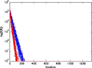
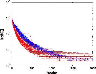
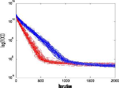
However, when the dimension D = 30, the standard PSO 2011 can achieve better optimization results for some benchmark functions than APEPSO according to Table 3. Moreover, since the standard PSO 2011 can achieve better optimization performance than PSOs with ring/full connection/scale free topologies, and APEPSO is derived from PEPSO and PEPSO II and it can achieve better optimization results than PEPSO and PEPSO II for the most of the benchmark functions and it does not need to choose the preferring possibility value or parameter, it will be fine to focus on the comparisons between APEPSO and standard PSO 2011, and it is better to draw the figures of time evolutions of the best fitness function values to find whether APEPSO is premature earlier than the standard PSO 2011. According to the simulations, the time evolutions of the best fitness function value are shown in Figures 2–8 about the benchmark function f1 to f7 when the dimension D=10. In Figures 2–8, there are 50 curves with the same colour related to the 50 trials for the standard PSO 2011 or APEPSO. It should be noted that the red lines are the results using the standard PSO 2011 and the blue lines are the results using APEPSO in Figures 2–16. To get a clear vision about the optimization process the log coordinate in y axis has been used for the time evolution figures except the figures with negative fitness values.

Time evolutions of the best fitness function value about Rastrigin function when D=10 (the red lines are the results using the standard PSO 2011 and the blue lines are the results using APEPSO for this figure and the following figures)
Time evolutions of the best fitness function value about Step function when D=10
Time evolutions of the best fitness function value about Rosenbrock function when D=10
Time evolutions of the best fitness function value about Salomon function when D=10
Time evolutions of the best fitness function value about Quartic function when D=10

Time evolutions of the best fitness function value about Shifted Griewank function when D=10 (To get a clear vision about the optimization process partial figure have been enlarged as the embedded figure).
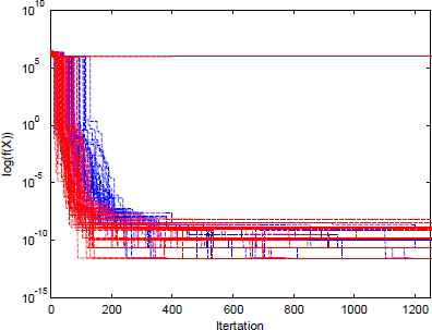
Time evolutions of the best fitness function value about Gear Train when D=10
According to Figures 2–8, APEPSO takes more time to reach its stable status especially Figures 2, 4 and 6, APEPSO is still in the process of achieving better results although the standard PSO 2011 has reached its mature stations for most of the tries, which means that the standard PSO 2011 is easier to be premature than APEPSO. The convergence of APEPSO is a little bit slower than the standard PSO 2011 because APEPSO takes more time to find the global best results without being trapped in the local minimums in a short time. When the dimension D = 30 the optimization performance for some benchmark functions are not better than the standard PSO 2011 according to Table 4, it is logical to assume this result is caused by the maximum number of function evaluations, which is set 20000 for every trial and may be not enough for APEPSO. To investigate whether this guess is correct, we set the maximum number of function evaluations as 40000 for every trial and other parameters are not changed; and the simulation results are listed in Table 4. According to the statistical results in Table 4, it proves our guess that the maximum number of function evaluations limited the optimization performance of APEPSO since the optimization performance has been improved with the increment of the maximum number of function evaluations.
| Problem | Method | best | Mean | Worst | Std.dev |
|---|---|---|---|---|---|
| Rastrigin function f8 | Standard PSO 2011 | 39.7983 | 90.6006 | 382.0256 | 54.2689 |
| APEPSO | 23.9677 | 77.4392 | 141.0321 | 32.6765 | |
| Step function f9 | Standard PSO 2011 | 0 | 18.74 | 611 | 87.85 |
| APEPSO | 0 | 0.62 | 3 | 0.7253 | |
| Rosenbrock function f10 | Standard PSO 2011 | 10.0945 | 300.3639 | 2.528e+003 | 543.1381 |
| APEPSO | 7.4338 | 120.3019 | 901.9223 | 172.2884 | |
| Salomon function f11 | Standard PSO 2011 | 0.1999 | 0.3019 | 0.4999 | 0.0714 |
| APEPSO | 0.1999 | 0.2323 | 0.2999 | 0.0469 | |
| Quartic function f12 | Standard PSO 2011 | 0.0083 | 0.0272 | 0.0887 | 0.0149 |
| APEPSO | 0.0048 | 0.0177 | 0.0443 | 0.0087 | |
| Shifted Griewank function f13 | Standard PSO 2011 | - 172.0213 | - 172.0213 | -172.0213 | 0 |
| APEPSO | - 172.0213 | - 172.0213 | -172.0213 | 0 |
Statistical results of SPSO 2011 and APEPSO when the maximum number of function evaluations is 40000 for every trial and the function dimension is 30
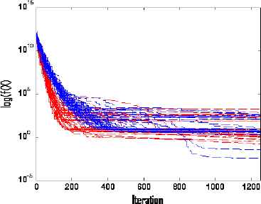
To check whether the APEPSO is ‘mature’ at the end of the optimization process, the time evolution figures of the best fitness function value have been shown in Figures 9–14. According to Figures 9–14, they further prove that APEPSO is not easy to be premature and can achieve better optimization results than standard PSO 2011.
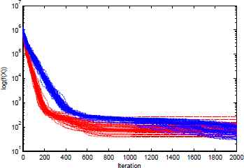
Time evolutions of the best fitness function value about Rastrigin when D=30 (APEPSO still has the trend to be achieve better optimization performance)
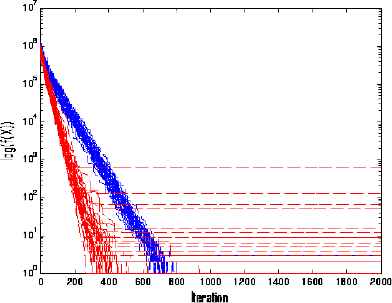
Time evolutions of the best fitness function value about Step function when D=30
Time evolutions of the best fitness function value about Rosenbrock function when D=30
Time evolutions of the best fitness function value about Salomon function when D=30
Time evolutions of the best fitness function value about Quartic function when D=30

Time evolutions of the best fitness function value about Shifted Griewank function when D = 30 (To get a clear vision about the optimization process partial figure have been enlarged as the embedded figure).
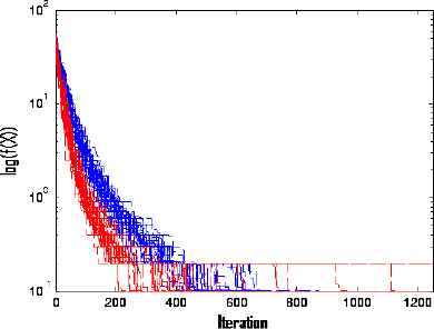
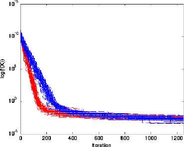
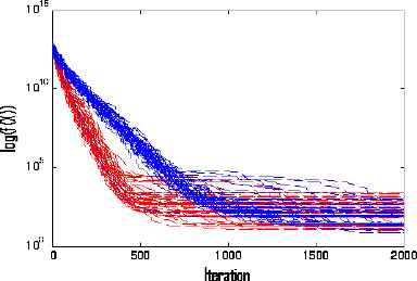
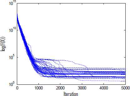
According to Figures 9 and 11, APEPSO may not achieve its potential. Hence we set the maximum number of function evaluations 100000 for every trial and do simulation for f8 and f10 based on APEPSO, and the results are shown in Table 5. Comparing Table 3 and 4, the optimization performance has been further improved when the maximum number of function evaluations is 100000 for every trial. The relevant time evolutions of the best fitness function value for f8 and f10 are shown in Figures 15 and 16, which meet the results of Table 4.

Time evolutions of the best fitness function value about Rastrigin function f8 with with a maximum number of function evaluations of 100000 for every trial (it shows that APEPSO is not easy to be premature)
Time evolutions of the best fitness function value about Rosenbrock function f10 with a maximum number of function evaluations of 100000 for every trial
| Problem | Method | best | Mean | Worst | Std.dev |
|---|---|---|---|---|---|
| Rastrigin function f8 | APEPSO | 12.9345 | 32.0719 | 95.3182 | 16.6891 |
| Rosenbrock function f10 | APEPSO | 3.8793 | 74.89.15 | 564.1397 | 97.2075 |
Results using APEPSO when the maximum number of function evaluations is 100000 for every trial
According to Figures 15 and 16, APEPSO keeps on searching and achieving better results although the process is approaching the last stage, especially in Figure 15, APEPSO is not mature, which shows that APEPSO can achieve better optimization result and does not need explicit topology information and no extra parameters need to be set.
5. Transmission network planning
Transmission network planning begins with the establishment of power demand growth scenarios, in accordance with forecasts along the time. Given these scenarios, one can verify the eventual need to broaden and to strengthen the network. In case electric service conditions are not satisfied, there should be proposed a plan that has coherence among the power supply availability, demand, and installation of new equipment in the network. Integration of these new equipment in the network, aimed at maintaining suitable technical and operating conditions, requires planning of the allocation of such reinforcement [20]. Main objective of the transmission expansion planning is to obtain the optimal expansion plan, while fulfilling operating and economic requirements. One classical transmission network expansion planning (TNEP), which does not consider the security constraints, is to determine the set of new lines to be constructed such that the cost of expansion plan is minimum and no overloads are produced during the planning horizon. A DC power flow based model is used for TNEP [20, 21]. The TNEP without security constraints can be stated as follows [20, 21],
Sf + g = d
fl and θl are unbounded
nl ≥ 0 and is integer for l ∈ 1,2……, nl
l ∈ Ω.
- cl:
cost of line added in lth right-of-way,
- S:
branch-node incidence transposed matrix of the power system,
- f:
vector with elements fl,
- γl:
susceptance of the circuit that can be added to lth right-of-way,
- nl:
the number of circuits added in lth right-of-way,
-
no. of circuits in the base case,
- Δθl:
phase angle difference in lth right-of-way,
- fl:
total real power flow by the circuit in lth right-of-way,
-
maximum allowed real power flow in the circuit in lth right-of-way,
-
maximum number of circuits that can be added in lth right-of-way,
- Ω:
set of all right-of-ways,
- nl:
total number of lines in circuit.
The transmission lines added in any right-of–way are the decision variables. The cost of each solution to the TNEP without security constraints can be obtained using the following function:
The objective of the TNEP is to find the set of transmission lines to be constructed such that the cost of expansion plan is minimum and no overloads are produced during the planning horizon. Hence, first term in the equation (9) indicates the total investment cost of a transmission expansion plan. The second term is added to the objective function for the real power flow constraint violations. The third term is added to the objective function if maximum number of circuits that can be added in lth right-of-way exceeds the maximum limit. W1, W2 are constants. The second and third terms are added to the fitness function only in case of violations.
We set the maximum number of function evaluations as 100000 for every trial and other parameters are not changed; and the simulation results are listed in Table 6. As can be seen from the Table 6, APEPSO achieved the optimal value and the statistical results, and it is proven that APEPSO can achieve better optimization results than SPSO in this application.
| Problem | Method | best | Mean | Worst | Std.dev |
|---|---|---|---|---|---|
| Transmission Network Expansion Planning Problem | Standard PSO 2011 | 220 | 234.54 | 323 | 24.1358 |
| APEPSO | 220 | 220 | 220 | 0 |
Results using the standard PSO 2011 and APEPSO for Transmission Network Expansion Planning Problem
6. Conclusion
This paper proposed three elitist set based particle swarm optimization algorithms, which are called 1) Probabilistic preference and Elitist set based Particle Swarm Optimization (PEPSO), 2) Probabilistic preference and Elitist set based Particle Swarm Optimization considering the individual two nearest experience neighbours (PEPSO II) and 3) Adaptive Probabilistic preference and Elitist set based Particle Swarm Optimization considering the individual two nearest experience neighbours (APEPSO). These methods do not need explicit topology structures, and an elitist set is used and based on the individual best experiences for the swarm communication. These three methods have been applied to several well-known benchmarks and achieved good optimization results. Among these three proposed algorithms, APEPSO can achieve better optimization performance than the standard PSO 2011 and some other PSOs with different topologies for all the benchmark functions and the application, and it does not need to turn the parameters. In the future, we will focus on the theoretic analysis of the proposed method.
Acknowledgement
The author declares that there is no conflict of interest regarding the publication of this paper. The author thanks the Matlab for the version codes of SPSO 2011 by Mahamed Omran, available on the particle swarm central website [8].
References
Cite this article
TY  - JOUR
AU  - Yanxia Sun
AU  - Zenghui Wang
PY  - 2017
DA  - 2017/09/14
TI  - Elitism set based particle swarm optimization and its application
JO  - International Journal of Computational Intelligence Systems
SP  - 1316
EP  - 1329
VL  - 10
IS  - 1
SN  - 1875-6883
UR  - https://doi.org/10.2991/ijcis.10.1.92
DO  - 10.2991/ijcis.10.1.92
ID  - Sun2017
ER  -