
Design of PID controller for sun tracker system using QRAWCP approach
- DOI
- 10.2991/ijcis.11.1.11How to use a DOI?
- Keywords
- PID controller; QRAWCP; Servo motor; Sun tracker; Wind disturbance
- Abstract
In this paper, a direct formula is proposed for design of robust PID controller for sun tracker system using quadratic regulator approach with compensating pole (QRAWCP). The main advantage of the proposed approach is that, there is no need to use recently developed iterative soft computing techniques which are time consuming, computationally inefficient and also there is need to know boundary of search space. In order to show the superiority of the proposed approach, performance of the sun tracker system is compared with the recently applied tuning approaches for sun tracker systems such as particle swarm optimization, firefly algorithm and cuckoo search algorithm. The performance of the existing and proposed approaches are verified in time domain, frequency domain and also using integral performances indices. It is found that the performance is improved in transient, robustness, and uncertainty aspects in comparison to recently proposed soft computing approaches.
- Copyright
- © 2018, the Authors. Published by Atlantis Press.
- Open Access
- This is an open access article under the CC BY-NC license (http://creativecommons.org/licences/by-nc/4.0/).
1. Introduction
In today’s technological era, electrical and electronic devices are developing rapidly. Therefore, the energy demand of every country is rising 1. Moreover, an important attention is also towards the environment. This requirement of energy has to be satisfied without polluting the environment, mainly by adopting renewable energy sources 3,2. It is available in different forms like wind power, hydro-power, solar energy, geothermal energy, bio-energy, etc. To utilize this energy, power plant has to be installed at suitable geographic location. In all these natural energy sources, solar energy plays a vital role. It is the fastest growing renewable source, as its installation cost is minimum as compared to other power plants and can be utilized at several places like within city or farm as well.
According to International Renewable Energy Agency (IRENA) capacity statistics of 2016 report 4, the total renewable energy generated around the world is 1,985,074 MW. Out of this, solar energy has generated 227, 010 MW and the actual requirement 5 till 2030 is 199,721 TW.h. Also according to 6, covering 0.16% of the land with 10% efficient solar conversion would reduce the worlds consumption rate of fossil fuel up to 200%. This statistics clearly indicates that efficient methodology is required to harness the solar energy. Keeping this fact in mind, it is necessary that solar energy should be captured properly through tracking control system. It is worth noting that the output efficiency could be improved from 40–50% if the solar tracking systems are designed well.
For solar power plant, the basic requirement is a solar panel which consists of photo voltaic (PV) cells. These panels are of different types like active, passive and time based solar tracker 6. The active solar trackers are of two types such as, single axis and dual axis 7. In single axis, only one angle is varied and other is fixed, whereas dual axis, is like a two degree of freedom (DOF) system. In this, one is an azimuth angle (θ) which is measured from clockwise rotation across the base and other is tilt angle (α) which is measured from incoming sunlight incidence to panel. This α is also known as elevation angle measured from horizon. In literature, it is found that an additional angle, i.e., zenith angle is also considered, which is measured from vertical direction. This is shown in Fig. 1.
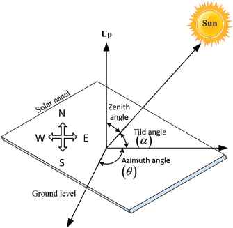
Different angles of sun tracker system
In passive tracker 8, the working principle is based on the imbalanced weights of cylindrical tubes. During the daytime, sunlight intensity varies, since pressure inside the tube and weight of the cylinder also varies. So accordingly solar panel also rotates. In a time based tracker system 9, first of all, sun position is recorded as per to daily or yearly experience. Further, this tracking data (co-ordinates) is programmed with the controller for future positions. In 10,1, researchers analyzed efficiency in terms of output power between fixed panel and solar tracker system. This results are carried on physical fix PV and solar tracker system which shows improvement in power output during different conditions like clear sky, partially clear sky, and cloudy sky which is improved to 18%, 14% and 13% respectively. In literature, sun trackers are controlled using PID, fuzzy 11, adaptive neural 12, ANFIS based proportional integral (PI) 13 and bio inspired PI controller 14. As we know that, even today also PID controller is used in industries 15. This PID is designed either based on analytically or graphical methods and also from past few decades stochastic optimization techniques 16. Various papers exist on tuning of PID controller 17. The first paper on PID tuning came in the literature in 1942 by Ziegler Nichols (ZN) 18. In this approach, the direct formula of deterministic approach is given for the tuning of PID parameters. The extension of this work is proposed by Cohen-Coon method in 1952 19, which is based on ZN technique along with dead time consideration. Recently, number of techniques has also been proposed and used in various applications such as process control 20, dcdc converters 21 and robustness for random perturbations 23,22. Similar to these analytical approach, graphical methods have been reported for tuning of PID parameters such as root locus, bode plot, stability boundary locus 25,24 etc.
It is observed that there are advancements in computer technology, hence mathematical computation power has increased a lot. It is found that from last few decades, stochastic optimization techniques are popular 26, in order to find optimal solution of PID type controllers. One such technique is swarm optimization which is based on swarm inspired behavior of birds and insects in our environment. One type of swarm optimization techniques is particle swarm optimization (PSO) which is proposed by Kennedy and Eberthart 28,27. It is based on behavior of birds which are searching for food in a group. Further, firefly algorithm (FFA) 29 is based on flashing behavior of fireflies which attract each other. Furthermore, cuckoo search algorithm (CSA) 30 is based on cuckoos behavior of laying eggs in another bird’s nest for hatching, but the probability is that, host bird may find the cuckoo’s egg and throw it out. Here, the cuckoo’s egg is the objective solution for the problem. In 31 optimal control technique is proposed, which is simple computational for convex system. In 32, it is shown that the optimal and robust PID controller can be designed using pole placement approach. The method has been applied to inverted pendulum problem. However, no direct formula is given for tuning of PID controller. Therefore, in this paper, a new method has been proposed for obtaining direct formula for designing PID controller using quadratic regulator approach with compensating pole (QRAWCP). The advantage of this method is that there is no need for any iterative procedure for designing of PID controller. The validity of the proposed approach is carried out by checking robustness and optimality. The results are compared with the recently proposed standard soft computing methods.
The rest of the paper is organized in the following manner: In section 2, parameters of the sun tracker system and its model are described. In section 3, QRAWCP approach to design PID controller is presented. In section 4, simulation results of proposed approach is presented. Finally, in the last section, conclusion and future scope are discussed.
2. Model of sun tracker system
In this paper, the sun tracker system with DC servo motor and PID controller is shown in Fig. 2. To obtain maximum efficiency from solar panel, minimum two axis of sun tracker is required, i.e., one is azimuth angle (θ) which measures the angle of incoming sunlight to the surface of PV cell and other is tilted angle (α) which measures the inclination angle of sunlight. As sun tracker is a non-interacting system, controller designed for single axis will be the replica for another axis also. Therefore, the analysis has been carried out on a single axis sun tracker system as shown in Fig. 3. Mathematical model of sun tracker is determined using basic laws of physics. For the major hardware parts such as DC servo motor, it’s speed transfer function G1 is given in (1) and G2 is for position control in (2). A gear ratio (N) and other parameters with values are listed in Table 1. Now considering single axis model as shown in Fig. 3. Applying Kirchhoff law to DC motor, we get velocity (ω(s)) control transfer function as
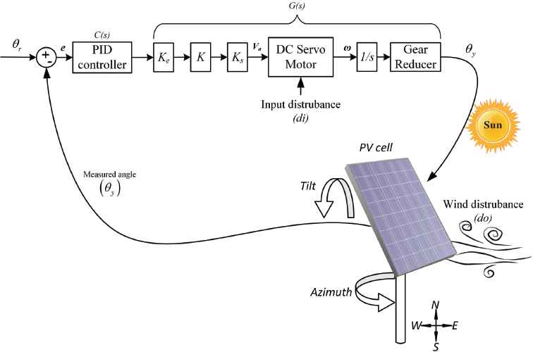
Control of sun tracker system layout

Model of sun tracking system
| Parameter | Value | Unit |
|---|---|---|
| Error discriminator(Ke) | 0.001 | V/rad |
| Amplifier gain(K) | 10000 | V/V |
| Servo amplifier(Ks) | 1 | V/V |
| Armature resistance(Ra) | 6.25 | ohm |
| Armature inductance(La) | 0.001 | H |
| Torque constant(Kt) | 0.01125 | Nm/A |
| Back emf constant(Kb) | 0.0125 | Nm/A |
| Inertia of motor rotor(J) | 1 × 10‒6 | kgm2/rad |
| Friction coefficient(b) | 0.000001 | Nm |
| Gear ratio(N) | 1/800 | - |
Parameters of sun tracker system
3. Proposed QRAWCP approach to design PID controller for sun tracker system
The quadratic regulator approach with compensation pole (QRAWCP) approach to tune PID controller is described as follows.
Step 1: The transfer function of the sun tracker system model G(s) is given in (4), and it’s parameters are given in Table 1. The proportional (Kp), integral (Ki) and derivative (Kd) (PID) controller C(s) can be written as
Step 2: The closed-loop characteristic equation for PID controller C(s) and plant G(s) is given as,
Simplifying (7) and equating to zero, we get,
Step 3: The state space form for sun tracker system is given in (5). Using this, design of PID by QRAWCP approach are given in step 4 to step 7. They are given below.
Step 4: Determination of performance index in terms of initial condition:
The quadratic regulator approach is an optimal state feedback controller which can be designed to minimize a specific quadratic cost function, also known as performance index (PI). The PI is designed for constraints like control voltage (u), output signal (y), error (e) or unconstrained objectives of linear time invariant (LTI) system. The optimal control vector u(t) is obtained by using the following equation:
Step 5: From (15), the minimization of Jl gives Kl by using feedback control law u = −Klx. The feedback gain Kl is found by using
In (19), Q and R are selected in such a way that Q = diag(q11, q22, q33) is q11 > q22 > q33 > 0 and R = χT χ > 0, where χ is non singular matrix.
Step 6: Using Riccati equation (19) and state model from (5), positive definite matrix P is obtained which is given below.
Step 7: Using (18), state feedback control gain Kl is obtained as
Step 8: Using state feedback control law for Ã, new system matrix can be written as,
From (23), the closed-loop characteristic equation can be written as
Step 9: The order of closed-loop system (8) is of fourth order and (24) is of third order. Therefore, in order to compare these two equations, we need to add one pole. The methodology of adding pole is explained below.
Let us consider fourth pole (s + λ4) on the left half of the s-plane. Then (24) can be written as,
The above (25) can also be written as
If (26) is compared with (8), λ4 is calculated as
The fourth pole (s + λ4) is augmented by δ. Here, δ is a compensation factor which is a variable value. Thus, modified λ4 becomes,
Step 10: By comparing (8) and (31), we get PID controller C(s) parameters as follows,
4. Simulation result and analyses
Using (4), substitute system parameters from Table 1 in (8). Further, Q and R are considered such that Q = diag [1, 1, 1] and R = 1 × 10⁻⁵. The gain matrix Kl can be calculated using (22), i.e., Kl = [7.9958, 13.8156, 316.2278]. The eigenvalues of closed loop system à becomes, λ1 = −6.2354 × 10³, λ2 = −23.5549, λ3 = −2.1530 × 10⁻³. The original system (24) is of third order. Therefore, we require one more pole which is calculated using (27), so we get λ4 = −1.2510 × 10⁴. Augmenting with δ = 10000 that gives λ4 = −2.5100 × 10³. Using these roots, the coefficients of characteristic equation (31) is obtained as: p1 = 8.7690 × 10³, p2 = 1.5857 × 10⁷, p3 = 3.6869 × 10⁸ and p4 = 7.9373 × 10⁵ Using (4), (20), then substituting in (32), we get QRAWCP PID controller parameters as Kp = 2.6218 × 10³, Ki = 5.6443, Kd = 111.7160.
4.1. Time response analysis
To validate the proposed technique and to show the superiority of QRAWCP approach, we analyze step response of sun tracker system for three cases, (i) without disturbance, (ii) with input disturbance and (iii) with output disturbance. The results are compared with the recently designed PID controller for sun tracker system which is based on swarm optimization approaches such as PSO 30, FFA 30 and CSA 30. The PID parameters of proposed QRAWCP PID and PSO PID, FFA PID, and CSA PID are given in Table 2.
| Method | Kp | Ki | Kd |
|---|---|---|---|
| QRAWCP PID (Proposed) | 2621.80 | 5.64430 | 111.721 |
| PSO PID | 9.51202 | 7.49203 | 0.00022 |
| FFA PID | 9.72083 | 7.44047 | 0.00010 |
| CSA PID | 9.99999 | 8.11378 | 0.00010 |
PID controller parameters
The performance of proposed PID controller and other existing PID controllers is presented in case 1, case 2 and case 3 for without disturbance, with input disturbance and with output disturbance, respectively.
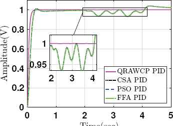
Case 1: Fig. 4 shows step response with controller for sun tracker system without disturbance. From this figure, it shows that performance of the proposed QRAWCP technique is better in comparison to other PID approaches which are based on soft computing technique.
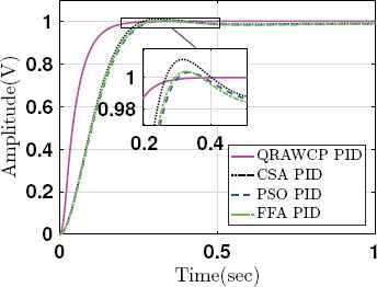
Step responses of system with PID controllers
The results are verified by calculating transient performance analysis such as, rise time (tr), settling time (ts), overshoot (Mp), absolute peak value (Atp), peak time (tp) and steady state error (ess). These are tabulated in Table 3. From this table, it is found that, the proposed approach shows improved results in comparison to other PIDs. Fig. 5 shows control signals using saturation limit of ±50V. It is found that overall control output of proposed QRAWCP approach is less in comparison to other techniques. The performance of proposed PID is verified for disturbance di(t) and do(t), where di(t) is input disturbance and do(t) is output disturbance. Both these disturbances are written mathematically in (33).
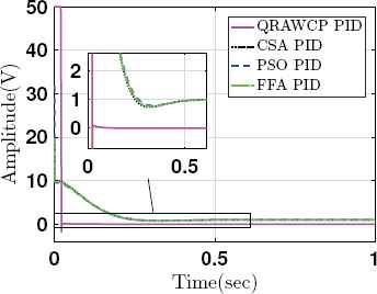
Control input response without disturbance
| Method | tr(sec) | ts(sec) | Mp(%) | At p | tp(sec) | ess |
|---|---|---|---|---|---|---|
| QRAWCP PID (Proposed) | 0.09490 | 0.17750 | 0.00011 | 1.00010 | 0.79410 | 0.00011 |
| PSO PID | 0.16640 | 0.25850 | 0.32890 | 1.00330 | 0.33550 | 0.01146 |
| FFA PID | 0.16300 | 0.25230 | 0.38740 | 1.00390 | 0.32720 | 0.01256 |
| CSA PID | 0.15670 | 0.23830 | 1.15880 | 1.01160 | 0.31580 | 0.00942 |
Output response of system
The output response of these equations are shown in Fig. 6. The performance analysis of the system in case of input disturbance and output disturbance is presented in case 2 and case 3, respectively.
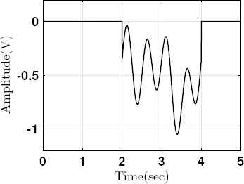
Disturbance (d(t)) applied to system
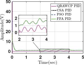
Case 2: Fig. 7 shows the step response of the system when the disturbance (di(t)) is applied from 2 to 4 seconds. The proposed approach gives better response in comparison to other PIDs. Fig. 8 shows control efforts which is quite higher for proposed controller at initial time. It is because of large inertia of system at initial time. However, during disturbance time 2 to 4 sec (see Fig. 8), we found that it is lesser and stable output (see Fig. 7) in comparison to other approaches.
Step responses of system with input disturbance
Control input responses with input disturbance
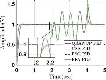
Case 3: Fig. 9 shows step response of system when output disturbance (do(t)) is applied from 2 to 4 sec. to the plant output side, i.e., the measurement noise. It is seen that, the proposed approach gives stable response with negligible ess in comparison to other PID approaches. The control efforts are shown in Fig. 10, which is quite higher for proposed QRAWCP PID controller. However, during disturbance time 2 to 4 sec, we found that, there is less overshoot in system output, whereas other approaches have large overshoot (see Fig. 9). Also, for safety purpose we have considered the saturation limit of ±50V. Further, loop robustness is also verified with controller which is given in following section.
Step responses of system with output disturbance
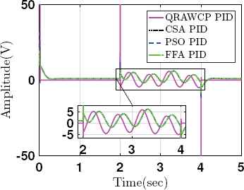
Control input responses with output disturbance
4.2. Loop robustness
The robustness of PID controllers for sun tracker system, to calculate loop transfer function L(s), is given by (34).
| Method | GM (dB) | ωgc(rad/s) | PM (deg) | ωpc(rad/s) | ||S||∞ | DM (sec) |
|---|---|---|---|---|---|---|
| QRAWCP PID (Proposed) | ∞ | 2359.10 | 69.2549 | 0.0004 | 1.2293 | 0.0005 |
| PSO PID | 57.8081 | 8.8371 | 69.9214 | 407.8013 | 1.2320 | 0.1381 |
| FFA PID | 56.8303 | 9.0061 | 69.6572 | 389.6705 | 1.2356 | 0.1350 |
| CSA PID | 56.5502 | 9.2369 | 68.8322 | 388.9042 | 1.2425 | 0.1301 |
Loop robustness of PID compensated system
Further, there is need to calculate sensitivity (||S||∞) and delay margin (DM) for robustness analysis 33. The sensitivity (S) can be calculated as,
It is observed that, proposed PID controller shows better stability margin, reduces delay margin, better sensitivity is compare to other methods. Finally, the comparative studies of proposed QRACWP approach with existing approaches30 are carried out by calculating integral performance indices. They are explained below.
4.3. Integral performance indices
The commonly used performance measures are Integral Squared Error (ISE), Integral Absolute Error (IAE) and Integral Time-weighted Absolute Error (ITAE). The mathematical form is given as
| Methods | Nominal case | ‒50% Lower bound | +50% Upper bound | ||||||
|---|---|---|---|---|---|---|---|---|---|
| ISE | IAE | ITAE | ISE | IAE | ITAE | ISE | IAE | ITAE | |
| QRAWCP PID (Proposed) | 0.0315 | 0.0532 | 0.0024 | 0.0583 | 0.0845 | 0.0048 | 0.0260 | 0.0474 | 0.0021 |
| PSO PID | 0.0755 | 0.1189 | 0.0137 | 0.2140 | 0.3409 | 0.0841 | 0.0464 | 0.1019 | 0.0232 |
| FFA PID | 0.0744 | 0.1180 | 0.0140 | 0.2110 | 0.3368 | 0.0824 | 0.0459 | 0.1016 | 0.0233 |
| CSA PID | 0.0727 | 0.1134 | 0.0123 | 0.2050 | 0.3280 | 0.0790 | 0.0450 | 0.0988 | 0.0218 |
Integral performance indices for 50% perturbation without disturbance
4.4. Parametric uncertainties
We know that in real time, parameters of the system are not constant. They vary from minimum to maximum value. This is primarily due to nonlinearity, environmental change and also due to ageing. The main objective of controller design is that it should work even though there exist uncertainties in the system. Here, for sun tracker system model, its parameters are represented in terms of uncertainties as
Similar to section 4.1, the performance analysis is carried out for both lower and upper bounds. From Fig. 11 and Fig. 12, it is observed that the performance of the proposed control is better in comparison to existing controllers except control input is slightly more at early part of the response. Further, performance in case of parametric uncertainly is carried out by determining performance indices in case of without and with input disturbances. They are shown in Table 5 and 6, respectively. Both these tables indicate that the proposed controller approach is better in comparison to existing controllers.
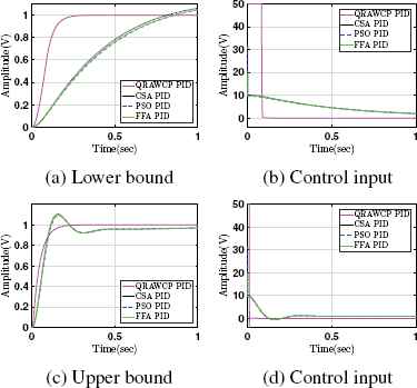
Response for 50% parametric uncertainties in system without disturbance

Response for 50% parametric uncertainties with input disturbance in system
| Methods | Nominal Plant | Lower ‒50% plant | Upper +50% plant | ||||||
|---|---|---|---|---|---|---|---|---|---|
| ISE | IAE | ITAE | ISE | IAE | ITAE | ISE | IAE | ITAE | |
| QRAWCP PID (Proposed) | 0.0315 | 0.0536 | 0.0037 | 0.0583 | 0.0850 | 0.0063 | 0.0260 | 0.0478 | 0.0033 |
| PSO PID | 0.0790 | 0.2166 | 0.3386 | 0.2275 | 0.5221 | 0.5004 | 0.0516 | 0.2250 | 0.3940 |
| FFA PID | 0.0779 | 0.2159 | 0.3371 | 0.2234 | 0.5114 | 0.4856 | 0.0510 | 0.2244 | 0.3913 |
| CSA PID | 0.0759 | 0.2043 | 0.3176 | 0.2185 | 0.5065 | 0.4831 | 0.0496 | 0.2138 | 0.3706 |
Integral performance indices for 50% perturbation with input disturbance
5. Conclusion
This paper deals with the direct formula for designing an optimal PID controller for sun tracking systems without using iterative and time consuming processes. In this regard, new QRAWCP approach is proposed for tuning of PID controller. It is shown that the proposed technique gives improved performance of sun tracking system in comparison to recent stochastic optimization methods like PSO, FFA and CSA in terms of transient response, loop robustness and integral error performance indices. The main objective of this paper is to indicate that in PID controller design applications, particularly for sun tracker system, there is no need to use recently developed, time consuming, soft computing techniques for PID controller design of sun tracker systems. Still, results based on fundamental control theory is better for designing of PID controller. In future, the proposed approach can be applied to various other engineering problems. Similarly, the work is in progress for developing the direct formula for finding optimal controller when there is parametric variations in the sun tracking systems.
References
Cite this article
TY  - JOUR
AU  - Sandeep D. Hanwate
AU  - Yogesh V. Hote
PY  - 2018
DA  - 2018/01/01
TI  - Design of PID controller for sun tracker system using QRAWCP approach
JO  - International Journal of Computational Intelligence Systems
SP  - 133
EP  - 145
VL  - 11
IS  - 1
SN  - 1875-6883
UR  - https://doi.org/10.2991/ijcis.11.1.11
DO  - 10.2991/ijcis.11.1.11
ID  - Hanwate2018
ER  -