
Dynamic composite decision-theoretic rough set under the change of attributes
- DOI
- 10.2991/ijcis.11.1.27How to use a DOI?
- Keywords
- Composite information table; Decision-theoretic rough set; Quantitative composite relation; Matrix; Incremental updating
- Abstract
In practical decision-making, we prefer to characterize the uncertain problems with the hybrid data, which consists of various types of data, e.g., categorical data, numerical dada, interval-valued data and set-valued data. The extended rough sets can deal with single type of data based on specific binary relation, including the equivalence relation, neighborhood relation, partial order relation, tolerance relation, etc. However, the fusion of these relations is a significant challenge task in such composite information table. To tackle this issue, this paper proposes the intersection and union composite relation, and further introduces a quantitative composite decision-theoretic rough set model. Subsequently, we present a novel matrix-based approach to compute the upper and lower approximations in proposed model. Moreover, we propose the incremental updating mechanisms and algorithms under the addition and deletion of attributes. Finally, experimental valuations are conducted to illustrate the efficiency of proposed method and algorithms.
- Copyright
- © 2018, the Authors. Published by Atlantis Press.
- Open Access
- This is an open access article under the CC BY-NC license (http://creativecommons.org/licences/by-nc/4.0/).
1. Introduction
The information table may involve various types of data, e.g., categorical data, numerical data, interval-valued data, set-valued data, etc. As a useful tool to describe the uncertain problems, the theory of rough sets can be utilized to tackle the different types of data by different binary relations. For instance, the traditional rough set model was proposed by Pawlak based on the equivalence relation to address the categorical dada 23. Hu et al. presented the neighborhood relation to characterize the similarity of two objects with numerical data 5. Guan et al. discussed the set-valued information systems with the tolerance relation 3. Qian et al. proposed the interval ordered information systems for attribute reduction and ordering rules extraction 24. However, most existing studies focus on single type of data with a simple binary relation under the static information table.
Decision-theoretic rough set (DTRS) is a general probabilistic rough set model32. By considering the misclassification cost, DTRS model provides a mathematical interpretation of thresholds based on Bayesian decision procedure. Recently, there are many interesting works in decision-making model1, 22, 9, 10, 31, 14, 13, 17, 15, 16, 40, 41, 18. The original DTRS model only can handle categorical data. Recently, many extended DTRS models are proposed to solve different types of data. Li et al. presented a neighborhood based on DTRS model with numerical data and discussed the minimum cost attribute reduction in proposed model 12. To directly deal with real-valued and interval-valued data, Zhao et al. introduced fuzzy and interval-valued fuzzy DTRS model39. Yang et al. studied weighted mean, optimistic and pessimistic multigranulation DTRS in incomplete information table27. Qian et al. proposed multigranulation DTRS25 for the fusion of different relations. However, these studies don’t consider the composite information table in DTRS. Actually, it is significant to characterize the objects in practical problem solving with the hybrid data. Moveover, multiple types of data may be changed in dynamic information environment, e.g., the addition and deletion of attributes or objects.
Recently, the incremental updating strategies have been widely researched in rough sets 7, 6, 19, 21, 20, 30, 4, 26, 38, 8. To efficiently obtain the useful acknowledge under the change of information system, we can propose the incremental updating methods to reduce the computational time in the theory of rough sets. Li et al. introduced the novel model to incrementally update the lower and upper approximations based on the characteristic relation under the change of attributes11. Zheng et al. developed a rough set and rule tree based incremental knowledge acquisition algorithm42. Yang et al. presented a unified framework of dynamic probabilistic rough sets, which can incrementally update three regions under fifteen situations of change29, further they proposed a unified model of sequential three-way decisions and multilevel incremental processing28. Furthermore, the hybrid data should be considered in real-world applications and it may vary in an information table. Zhang et al. investigated the definition of composite information table and proposed a composite rough set model to deal with the different types of data simultaneously36. Then, they further provided a parallel matrix-based approach for computing composite rough set approximations 37. Chen et al. proposed the distribution attribute reduction method under probabilistic composite rough set2. However, the composite relation defined by the intersection operation of relations is too strict for classification problems. In this paper, we define a novel quantitative composite relation w.r.t. multiple types of data. We provide the matrix-based method to compute lower and upper approximations. Furthermore, we propose the incremental approach for updating approximations when the attributes are added or deleted in composite information table. Experiments on four datasets show that the incremental algorithms can efficiently improve the performance of approximations update.
The rest of this paper is organized as follows. Section 2 briefly reviews some basic notions and concepts of DTRS model. In Section 3, we propose a quantitative composite DTRS model based on the quantitative composite relation and further introduce a novel matrix-based approach for the calculation of approximations. Section 4 presents the incremental updating mechanisms and algorithms with composite DTRS model when the attributes are added or deleted in composite information table. Finally, experiments are conducted in Section 5 and Section 6 concludes the paper and elaborates on further works.
2. Decision-theoretic rough sets
Based on well-known Bayesian decision theory, DTRS model provides a mathematical approach for computing thresholds in probabilistic rough sets under the minimum decision risk or cost. In this section, we briefly review the basic concepts and notions of DTRS model 32,34.
Definition 1.
Let SS = (U,A = C ∪ D, V, f) be a single information table, where U is a nonempty finite set of objects; A is also a nonempty finite set, called the attributes of objects, C denotes the condition attributes set, which consists of a single type data, D denotes decision attribute set, C∩D = ∅; V is a domain of the attributes,
In a single information table, the type of data with respect to the condition attributes is same. The traditional rough sets commonly deal with such data. Given an approximation space (U, R). R is an equivalence relation on U, B ⊆ C, RB = {(x, y) ∈ U × U|∀b ∈ B, f (x, b) = f (y, b)}. U/R denotes a partition of U induced by the equivalence relation R. In Pawlak rough sets model, for X ∈ U, the lower and upper approximations can be denoted as:
Based on bayesian decisions rules, we usually make the optimized decisions with the minimum risk. For simplicity, we consider two states and three actions in a binary classification problem. The set of states is given by Ω = {X, XC} indicating that an element is in X and not in X, respectively. Under two opposite states, the set of actions is given by AC = {aP, aB, aN}, where aP, aB, aN represent the three actions in classifying an object, deciding POS(X), deciding BND(X) and deciding NEG(X). For cost-sensitive learning, the loss function contained six parameters is presented as the matrix L3×2 shown in Table 1.
| X(P) | XC(N) | |
|---|---|---|
| aP | λPP | λPN |
| aB | λBP | λBN |
| aN | λNP | λNN |
The loss function
In the matrix, λPP, λBP and λNP denote the losses incurred for taking actions of aP, aB and aN, respectively, when an object belongs to X. Similarly, λPN, λBN and λNN denote the losses incurred for taking the same actions when the object belongs to XC. The expected losses associated with taking the three actions can be expressed as:
Based on minimum-cost decision rules in the Bayesian decision procedure, the (α, β) lower and upper approximations of DTRS model can be defined by:
3. Composite decision-theoretic rough sets and matrix representation of approximations
3.1. Quantitative composite DTRS model
In general, the previous DTRS model can deal with the single data type in a single information table. However, hybrid data types usually appear in a composite information table, which contains categorical data, numerical data, set-valued data, interval-valued data, etc. We can utilize different binary relations to handle different types of data. In what follows, we introduce the definition of composite information table, and present the composite binary relation by fusion strategy in DTRS model.
Definition 2.
Let CS = (U, A = C∪D, V, f) be a composite information table, where U is a nonempty finite set of objects; A is also a nonempty finite set, called the attributes of objects, C denotes the condition attributes set consisted of hybrid type data, C = ∪Ck,k = 1, 2, …, m, where Ck is a subset of C with the same data type and m denotes the number of data types, D denotes decision attribute set, C∩D = ∅; V is a domain of the attributes,
Example 1.
In Table 2, there are four types of data in a composite information table CS = (U, A = C∪D, V, f). Let B = C = ∪Bk, k = 1, 2, 3, 4, where B1 = {bcategorical}, B2 = {bnumerical}, B3 = {binterval–valued}, B4 = {bset–valued}, D = {dcategorical}, denote categorical data, numerical data, interval-valued data, set-valued data, categorical data, respectively.
| U | bcategorical | bnumerical | binterval–valued | bset–valued | dcategorical |
|---|---|---|---|---|---|
| x1 | 1 | 0.4 | [1.2 1.5] | {1, 2} | 1 |
| x2 | 1 | 0.2 | [1.4 1.8] | {0, 1, 2} | 1 |
| x3 | 2 | 0.2 | [1.5 2.2] | {1} | 0 |
| x4 | 1 | 0.5 | [1.6 2.1] | {1, 3} | 1 |
| x5 | 2 | 0.2 | [1.4 1.7] | {1, 2, 3} | 0 |
| x6 | 1 | 0.4 | [2.2 2.5] | {3} | 1 |
A composite information table
For classification and decisions in such information table, the key issue is the fusion of different binary relations. Based on existing studies 36, we introduce three approaches to define the composite relation, namely, the intersect composite relation, the union composite relation, and the quantitative composite relation.
Definition 3.
Let CS = (U, A = C∪D, V, f) be a composite information table, where U = {x1, x2,···,xn}, X be a subset of U. B = ∪Bk ⊆ C, Bk ⊆ Ck. The characteristic matrix
Definition 4.
Let CS = (U, A = C∪D, V, f) be a composite information table, where U = {x1, x2, …, xn}, B = ∪Bk ⊆ C, Bk ⊆ Ck. The relation matrix MRBk = (mij)n×n can be defined as follows:
Definition 5. 36
(The intersect composite relation) Given a composite information table CS = (U,A = C∪D,V, f). Let x, y ∈ U and B = ∪Bk ⊆ C, Bk ⊆ Ck, the intersect composite relation
Similarly, we can define the union composite relation as follows.
Definition 6.
(The union composite relation) Given a composite information table CS = (U,A = C∪D, V, f). Let x, y ∈ U and B = ∪Bk ⊆ C, Bk ⊆ Ck, the union composite relation
In a composite information table, we present the intersection composite relation
Definition 7.
(The quantitative composite relation) Given a composite information table CS = (U A = C∪D, V, f). Let x, y ∈ U and B = ∪Bk ⊆ C, Bk ⊆ Ck,k = 1, 2,···,m. Suppose threshold θ satisfied 0 ⩽ θ < 1, the quantitative composite relation QCRB is defined as:
Definition 8.
Let CS = (U, A = C∪D,V, f) be a composite information table, QCRB be a quantitative composite relation. Suppose X ⊆ U, the (α, β) lower and upper approximations of concept X in composite DTRS model can be defined by:
The (α, β) probabilistic three regions are given as follows:
Definition 9.
Let CS = (U, A = C∪D,V,f) be a composite information table, QCRB be a quantitative composite relation. Let U/D = {D1,D2,···,Di,···,Ds} be a partition of U based on the decision attribute d. Then the (α, β) lower and upper approximations of the decision class Di in composite DTRS model can be defined by:
Example 2.
(Continuation of Example 1) In table 2, to deal with four types of data, four binary relations, namely, the equivalence relation, the neighborhood relation, the partial order relation, and the tolerance relation are given as follows:
- 1.
The equivalence relation (see definition in Section 2)
- 2.
The neighborhood relation
where - 3.
The partial order relation
- 4.
The tolerance relation
Suppose neighborhood threshold δ = 0.1. According to four definitions of binary relations, we can calculate four relation matrices with respect to four types of data respectively on U as follows:
3.2. Matrix representation of approximations
In order to propose a fast matrix-based approach for updating approximations under the change of attributes, another representation of approximations35 in DTRS model is given as follows.
Definition 10.
Let CS = (U, A = C∪D, V, f) be a composite information table, QCRB be a quantitative composite relation. Suppose X ⊆ U, the (α′, β′) lower and upper approximations of concept X in composite DTRS model can be defined by:
Definition 11.
Let Mn×1 be a matrix. The cut matrices of M↑ and M↓ are defined respectively as:
Definition 12.
Let CS = (U,AT = C∪D,V,f) be a composite information table, QCRB be a quantitative composite relation, where U = {x1, x2,···,xn}.
| Input: A composite information table CS = (U, A = C∪D, V, f), the concept X(X ⊆ U), and the loss function L3×2. |
|
Output: The characteristic matrices of lower and upper approximations
|
|
Step 1: Construct the characteristic matrix
|
|
Step 2: Compute the equivalence relation matrix
|
| Step 3: Compute the quantitative composite relation matrix MQCRB according to Definition 7 ; |
| Step 4: Compute the intersection matrix W = (wi)n × 1 = MQCRB * E and the non-intersection matrix W′ = (w′i)n × 1 = MQCRB * (∼E) |
|
Step 5: Compute the characteristic matrix of lower approximations
|
|
Step 6: Compute the characteristic matrix of upper approximations
|
(NCDTRS) The matrix-based algorithm for computing approximations in composite DTRS model.
Example 3.
(Continuation of Example 2) Suppose the loss function L = [0 6;1 3;5 0]. Then we have α′ = 3, β′ = 0 75. The lower approximation of composite DTRS model based on the matrix approach can be calculated as:
Similarity, the upper approximation of composite DTRS model based on the matrix approach can be calculated as:
4. The approach for incremental updating approximations under the change of attributes
In an dynamic composite information table, the change of attributes have two situations. One is the addition of attributes and another is the deletion of attributes. To achieve a fast calculate process, incremental updating the quantitative composite relation matrix and the characteristic matrices of approximations are two importance tasks. In this section, we introduce the incremental updating of matrix-based strategy in composite DTRS model.
4.1. updating the quantitative composite relation matrix and the characteristic matrices of approximations when adding attributes
In this subsection, the incremental update of approximations is considered as from time t to t + 1. Let CSt = (Ut, At = Ct∪Dt, Vt, ft) be the composite information table at time t, where U = {x1,x2,...,xn}. The composite information table CSt = (Ut, At = Ct ∪Dt, Vt, ft) at time t only contains four types of data, where Ct = Bt1 ∪Bt2 ∪Bt3∪Bt4, Bt1 denotes categorical data, Bt2 denotes numerical data, Bt3 denotes set-valued data, Bt4 denotes interval-valued data. Let CSt+1 = (Ut+1, At+1 = Ct+1 ∪Dt+1, Vt+1, ft+1) be the composite information table at time t + 1, where U = {x1,x2,...,xn}. At time t + 1, a set of attributes ΔC are added into CSt+1 = (Ut+1, At+1 = Ct+1∪Dt+1, Vt+1, ft+1), ΔC = ΔB1 ∪ΔB2 ∪ΔB3 ∪ΔB4, Ct+1 = Ct ∪ΔC.
From time t to t + 1, there are two steps to update the quantitative composite relation matrix. Step 1 is updating the equivalence relation matrix
Proposition 1.
Let CS = (U,A = C∪D, V, f) be a composite information system, where U ={x1,x2,...,xn}.
Proposition 2.
Let CS = (U,A = C∪D, V, f) be a composite information system, where U = {x1,x2,...,xn}.
Proposition 3.
Let CS = (U,A = C∪D, V, f) be a composite information system, where U = {x1,x2,...,xn}.
Proposition 4.
Let CS = (U,A = C∪D, V, f) be a composite information system, where U = {x1,x2,...,xn}.
Proposition 5.
Let CS = (U,A = C∪D, V, f) be a composite information system, where U = {x1,x2,...,xn}. MQRCB is the quantitative composite relation matrix on U. Suppose ΔC = ΔB1∪ΔB2 ∪ΔB3 ∪ΔB4, Ct+1 = Ct∪ΔC, the quantitative composite relation matrix MQRCB by adding ΔC to C from time t to t + 1 can be updated as:
Proposition 6.
Let CS = (U,A = C∪D, V, f) be a composite information system, where U = {x1,x2,...,xn}. MQRCB is the quantitative composite relation matrix on U. W = (wi)n×1 = MQCRB * E is the intersection matrix, and W′ = (w′i)n×1 = MQCRB * (~ E) is the non-intersection matrix, i = 1,2,...,n. Suppose ΔC = ΔB1∪ΔB2 ∪ΔB3 ∪ΔB4,Ct+1 = Ct∪ΔC. The intersection matrix W = (wi)n×1 = MQCRB * E can be updated as:
The incremental algorithm for computing approximations in composite DTRS model based on matrix when adding attributes is outlined in Algorithm 2 . Step 1 is to update four relation matrices according to Proposition 1–4, whose time complexity is O(|U|2). Step 2 is to updating quantitative relation matrix according to Proposition 5, whose time complexity is O(|U|2). Step 3 is to update W and W′ according to Proposition 6, whose time complexity is O(|U|2). Step 4 and Step 5 are to compute the characteristic matrices of lower and upper approximations, whose time complexity is O(|U|).
|
Input: At time t, a composite information table CSt = (Ut, At = Ct∪Dt, Vt, ft), the loss function L3×2, the characteristic matrix
|
|
Output: The characteristic matrices of lower and upper approximations
|
|
Step 1: Updating
|
| Step 2: Updating MQCRB according to Proposition 5; |
| Step 3: Updating W and W′ according to Proposition 6; |
| Step 4: Compute
the characteristic matrix of lower approximations
|
| Step 5: Compute
the characteristic matrix of upper approximations
|
(ICDTRS-AA) The incremental algorithm for computing approximations in composite DTRS model based on matrix when adding attributes.
4.2. updating the quantitative composite relation matrix and the characteristic matrices of approximations when deleting attributes
In this subsection, the incremental update of approximations is considered as from time t to t + 1. Let CSt = (Ut, At = Ct∪Dt, Vt, ft) be the composite information table at time t, where U = {x1,x2,...,xn}. The composite information table CSt = (Ut, At = Ct∪Dt, Vt, ft) at time t only contains four types of data, where Ct = Bt1∪Bt2∪Bt3∪Bt4, Bt1 denotes categorical data, Bt2 denotes numerical data, Bt3 denotes set-valued data, Bt4 denotes interval-valued data. Let CSt+1 = (Ut+1, At+1 = Ct+1 ∪Dt+1, Vt+1, ft+1) be the composite information table at time t + 1, where U = {x1,x2,...,xn}. At time t + 1, a set of attributes ΔC are deleted from CSt+1 = (Ut+1, At+1 = Ct+1∪Dt+1, Vt+1, ft+1), ΔC = ΔB1∪ΔB2∪ΔB3∪ΔB4, Ct+1 = Ct – ΔC.
Proposition 7.
Let CS = (U,A = C∪D, V, f) be a composite information system, where U = {x1,x2,...,xn}.
Proposition 8.
Let CS = (U,A = C∪D, V, f) be a composite information system, where U = {x1,x2, …, xn}.
Proposition 9.
Let CS = (U,A = C∪D, V, f) be a composite information system, where U = {x1,x2,...,xn}.
Proposition 10.
Let CS = (U,A = C∪D, V, f) be a composite information system, where U = {x1,x2,...,xn}.
Proposition 11.
Let CS = (U,A = C∪D, V, f) be a composite information system, where U = {x1,x2,...,xn}. MQRCB is the quantitative composite relation matrix on U. Suppose ΔC =ΔB1∪ΔB2∪ΔB3∪ΔB4, Ct+1 = Ct – ΔC, the quantitative composite relation matrix MQRCB by adding ΔC to C from time t to t + 1 can be updated as:
Proposition 12.
Let CS = (U,A = C∪D, V, f) be a composite information system, where U = {x1,x2,...,xn}. MQCRB is the quantitative composite relation matrix on U. W = (wi)n×1 = MQCRB* E is the intersection matrix, and W′ = (w′i)n × 1 = MQCRB * (∼ E) is the non-intersection matrix, i = 1,2,...,n. Suppose ΔC = ΔB1∪ΔB2 ∪ΔB3 ∪ΔB4, Ct+1 = Ct – ΔC. The intersection matrix W =(wi)n×1 = MQCRB* E can be updated as:
The incremental algorithm for computing approximations in composite DTRS model based on matrix when deleting attributes is outlined in Algorithm 3 . Step 1 is to update four relation matrices according to Proposition 5–8, whose time complexity is O(|U|2). Step 2 is to updating quantitative relation matrix according to Proposition 9, whose time complexity is O(|U|2). Step 3 is to update W and W′ according to Proposition 10, whose time complexity is O(|U|2). Step 4 and Step 5 are to compute the characteristic matrices of lower and upper approximations, whose time complexity is O(|U|).
|
Input:
At time t, a composite information table CSt = (Ut, At = Ct∪Dt, Vt, ft), the loss function L3×2, the characteristic matrix
|
|
Output:
The characteristic matrices of lower and upper approximations
|
|
Step 1: Updating
|
| Step 2: Updating MQCRBaccording to Proposition 9; |
| Step 3: Updating W and W′ according to Proposition 10; |
| Step 4: Compute
the characteristic matrix of lower approximations
|
| Step 5: Compute
the characteristic matrix of upper approximations
|
(ICDTRS-DA) The incremental algorithm for computing approximations in composite DTRS model based on matrix when deleting attributes.
5. Experimental evaluations
In this section, we conduct the comparative experiments to verify the performance of the proposed algorithms for incremental updating approximations in composite DTRS model when the attributes are changed. We elect two datasets from the machine learning data repository, University of California at Irvine (UCI) (http://archive.ics.uci.edu/ml/). One is the categorical data and another is the numerical data. Moreover, we generate two composite datasets, which contain four data types, namely, categorical data, numerical data, set-valued data, interval-valued data. The detailed datasets are shown in Table. All experiments were performed on a computer with Microsoft Windows 10, Inter (R) Core (TM) i5-4210U CUP @ 2.40 GHz and 12.0 GB of memory and the programming language is MATLAB R2016a.
5.1. A comparison of experiments when adding attributes
We divide four datasets into ten equal size of subsets respectively according to the number of attributes. At each datasets, the first five subsets is the original dataset, and the rest five subsets is the added datasets. We set five ratios for adding datasets, namely, 20% 40% 60% 80% 100%. The comparison of experimental results between Algorithm NCDTRS and Algorithm ICDTRS-AA are shown in Figure 1.
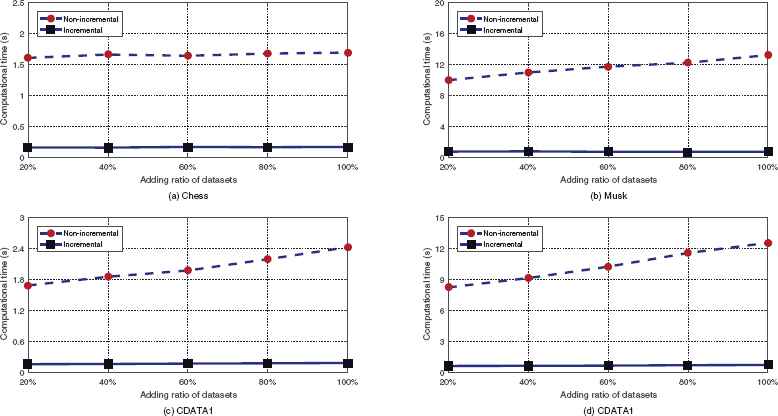
Comparison of non-incremental and incremental algorithms versus adding different ratios of attributes.
In Figure 1, we can observe that the computational time with respect to Algorithm NCDTRS and Algorithm ICDTRS-AA all increase with addition of attributes. However, it is easy to see that the computational time of incremental algorithm is less than the one of non-incremental algorithm in each sub-figure of figure 1. Furthermore, the bigger the datasets, more efficient the performance of incremental algorithm will be.
To further show the advantage of the incremental algorithm ICDTRS-AA, we calculate the incremental speedup, which denotes the ratios between the computational time of non-incremental algorithm and the one of incremental algorithm in Table 4. It is easy to see that the incremental speedup of four datasets in Table 3 is greater than one.
| Datesets | Objects | Class | Attributes | ||||
|---|---|---|---|---|---|---|---|
| Categorical | Numerical | Set-valued | Interval-valued | Total | |||
| Chess (King-Rock vs.King-Pawn) | 3196 | 2 | 36 | 0 | 0 | 0 | 36 |
| Musk (Version 2) | 6598 | 2 | 0 | 168 | 0 | 0 | 168 |
| CDATA1 | 3000 | 2 | 10 | 10 | 10 | 10 | 40 |
| CDATA2 | 6000 | 2 | 20 | 20 | 20 | 20 | 80 |
The description of datasets
| Datesets | The added ratios of attributes | ||||
|---|---|---|---|---|---|
| 20% | 40% | 60% | 80% | 100% | |
| Chess (King-Rock vs.King-Pawn) | 10.1067 | 10.5190 | 9.7336 | 10.2247 | 10.0106 |
| Musk (Version 2 | 13.4140 | 14.1118 | 16.2100 | 17.0289 | 18.1688 |
| CDATA1 | 10.2584 | 10.9947 | 11.1742 | 12.1243 | 12.8600 |
| CDATA2 | 12.5924 | 13.6767 | 14.9453 | 15.9917 | 16.8302 |
The incremental speedup versus adding the different radios of attributes
5.2. A comparison of experiments when deleting attributes
Similarly to the experimental methods in subsection 5.1, we also divide each dataset into ten equal size of subsets respectively according to the number of attributes. At each datasets, all ten subsets is the original dataset. We delete one subsets step by step from the original datasets. We set five ratios for deleting datasets, namely, 10% 20% 30% 40% 50%. The comparison of experimental results between Algorithm NCDTRS and Algorithm ICDTRS-DA are shown in Figure 2.
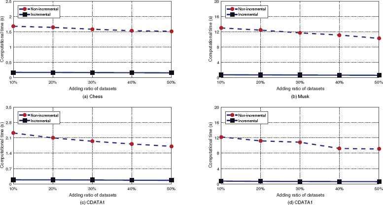
Comparison of non-incremental and incremental algorithms versus deleting different ratios of attributes.
In Figure 2, it is observed that the computational time with respect to Algorithm NCDTRS and Algorithm ICDTRS-DA all decrease with deletion of attributes. However, we can find that the computational time of incremental algorithm is less than the one of non-incremental algorithm in each sub-figure of figure 2. To further show the advantage of the incremental algorithm ICDTRS-DA, we calculate the incremental speedup, which denotes the ratios between the computational time of non-incremental algorithm and the one of incremental algorithm in Table 5. It is easy to see that the incremental speedup of four datasets in Table 3 is greater than one.
| Datesets | The deleted ratios of attributes | ||||
|---|---|---|---|---|---|
| 10% | 20% | 30% | 40% | 50% | |
| Chess (King-Rock vs.King-Pawn) | 10.0012 | 9.9005 | 9.8218 | 9.7104 | 9.8074 |
| Musk (Version 2 | 18.1741 | 18.1528 | 18.1931 | 18.1667 | 17.2593 |
| CDATA1 | 12.5081 | 11.5049 | 11.0677 | 10.8165 | 10.5514 |
| CDATA1 | 16.9251 | 17.1266 | 17.4265 | 15.3336 | 15.5728 |
The incremental speedup versus deleting the different radios of attributes
6. Conclusions
In this paper, we investigated the composite information table, which contains various types of data. We proposed the quantitative composite relation for fusion of multiple binary relations. Based on such composite relation, we introduced a quantitative composite DTRS model and provided a novel matrix-based approach to compute approximations. Moreover, to reduce running time w.r.t. the computation of the upper and lower approximations, the increase learning methods based on matrix updating strategy are presented in composite DTRS model versus the addition and deletion of attributes respectively. Experiment results show that the incremental algorithms are more efficient and effective to update approximations in composite DTRS model. Our future work will focus on the incremental updating mechanisms when objects are added or deleted in the composite information system.
Acknowledgments
This work is supported by the national science foundation of China (Nos. 61573292, 61572406, 61603313, 61602327, 71571148). The authors would like to thank Professor Yiyu Yao for useful comments on this study.
References
Cite this article
TY  - JOUR
AU  - Linna Wang
AU  - Xin Yang
AU  - Yong Chen
AU  - Ling Liu
AU  - Shiyong An
AU  - Pan Zhuo
PY  - 2018
DA  - 2018/01/01
TI  - Dynamic composite decision-theoretic rough set under the change of attributes
JO  - International Journal of Computational Intelligence Systems
SP  - 355
EP  - 370
VL  - 11
IS  - 1
SN  - 1875-6883
UR  - https://doi.org/10.2991/ijcis.11.1.27
DO  - 10.2991/ijcis.11.1.27
ID  - Wang2018
ER  -