
Fault diagnosis of sucker rod pumping systems based on Curvelet Transform and sparse multi-graph regularized extreme learning machine
- DOI
- 10.2991/ijcis.11.1.32How to use a DOI?
- Keywords
- curvelet transform; extreme learning machine; sparse representation; sucker rod pumping systems; fault diagnosis
- Abstract
A novel approach is proposed to complete the fault diagnosis of pumping systems automatically. Fast Discrete Curvelet Transform is firstly adopted to extract features of dynamometer cards that sampled from sucker rod pumping systems, then a sparse multi-graph regularized extreme learning machine algorithm (SMELM) is proposed and applied as a classifier. SMELM constructs two graphs to explore the inherent structure of the dynamometer cards: the intra-class graph expresses the relationship among data from the same class and the inter-class graph expresses the relationship among data from different classes. By incorporating the information of the two graphs into the objective function of extreme learning machine (ELM), SMELM can force the outputs of data from the same class to be as same as possible and simultaneously force results from different classes to be as separate as possible. Different from previous ELM models utilizing the structure of data, our graphs are constructed through sparse representation instead of K-nearest Neighbor algorithm. Hence, there is no parameter to be decided when constructing graphs and the graphs can reflect the relationship among data more exactly. Experiments are conducted on dynamometer cards acquired on the spot. Results demonstrate the efficacy of the proposed approach for faults diagnosis in sucker rod pumping systems.
- Copyright
- © 2018, the Authors. Published by Atlantis Press.
- Open Access
- This is an open access article under the CC BY-NC license (http://creativecommons.org/licences/by-nc/4.0/).
1. Introduction
Sucker rod pumping systems are the most common artificial lift methods used for oil production. Nearly 90% artificially lifted wells in the world1 and nearly 94% artificially lifted wells in China2 adopt sucker rod pumping systems. In production practice, sucker rod pumping systems are not stable and many kinds of faults can cause reduction of oil production, stop production and even damage to equipments. Therefore, diagnosing the faults of suck rod pumping systems automatically has been a very important research subject.
Many advanced methods have been adopted to overcome this problem. J.P. Wang, Z.F. Bao3 used a rough classifier to diagnosis faults. Y.H. He et al4 transferred the time domain signals into the frequency domain signals and used a fuzzy mathematical recognition model for diagnosis of failures in pumping wells. P. Xu et al5 constructed a self-organizing competitive neural network model to achieve automatization of fault diagnosis. W. Wu et al6 decomposed cards to get eight energy eigenvectors by using three layers of wavelet packet, and then regard them as the input of the RBF networks. K. Li et al7 used the moment curve method to extract the features of typical dynamometer cards and then used the improved SVM method for pattern classification. These researches show that fault diagnosis of sucker rod pumping systems can be regarded as a process of pattern recognition.
Feature extraction and the pattern classification are two important factors in pattern recognition problems. For sucker rod pumping systems, different working conditions can be represented by the shapes of dynamometer cards. Furthermore, the differences among dynamometer cards are mainly reflected in the scales and the directions. Curvelet Transform is a multi-resolution method which has been widely used to handle feature extraction problems8,9,10. It is not only a multi-scale but also a multi-direction transform, so features extracted by Curvelet Transform are very sensitive to the shapes of dynamometer cards. In this paper, Fast Discrete Curvelet Transform (FDCT) is adopted to extract features of dynamometer cards.
After feature extraction, an appropriate model should be chosen to classify the dynamometer cards. Extreme Learning Machine (ELM) proposed by G.B. Huang et al11 is a non-iterative method that has been proven to be an efficient model for classification. Many efforts have been made to improve the performance of ELM. Recently, using the data’s inherent structure detected by manifold learning algorithms12,13,14,15 to improve the performance of existing machine learning methods has drawn much attention16,17,18,19. Y. Peng et al20 used the K-nearest Neighbor algorithm (KNN) to construct the graphs and introduce the discriminative information into the ELM model to improve the performance, but how to choose the value of the parameter k in KNN is still a problem. Motived by Sparsity preserving projection21 and Graph regularized sparsity discriminant analysis22, we propose a sparse multi-graph regularized extreme learning machine (SMELM) for classification. In SMELM, two graphs: intra-class graph and inter-class graph are constructed to utilize the inherent structure of the training data more effectively. The intra-class graph can reflect the similarity among data in the same class; the inter-class graph can reflect the relationship among data from different classes. These two graphs help to improve the performance by forcing the output results of data from same class to be as same as possible and meanwhile forcing results from different classes to be as different as possible. Different from discriminative graph regularized extreme learning machines23, the sparse representation algorithm is used instead of the KNN algorithm, so there is no parameter to be decided when constructing graphs and the elements in graph matrix are not simplify set as 0 or 1. The graph matrix calculated by sparse representation can reflect the relationship among data more exactly so that the proposed SMELM can achieve better performance.
2. Dynamometer card feature extraction based on Discrete Curvelet
2.1. Dynamometer card and its properties
The dynamometer card is a closed curve of load versus displacement. Different working conditions of sucker rod pumping systems can be represented by the shapes of the dynamometer cards. For examples, the condition ”normal operation pump” is reflected by a closed curve of approximate parallelogram; the lower left corner of ”hitting bottom” has an extra circular pattern; for ”travelling valve leakage”, the upper portion of the curve is like a parabola; on the contrary, for ”standing valve leakage”, its shape is a downward arch; The curves of ”feed liquid failure” lack the right-bottom corner; and for ”sucker rod breakage”, its shape is a flat strip curve. Some main reference patterns of conditions are shown in Fig. 1. It can be seen that the differences among dynamometer cards of different conditions are obvious. Therefore, recognizing the shapes of dynamometer cards can distinguish the normal and fault conditions.

Classes of dynamometer card patterns.
2.2. Fast Discrete Curvelet Transform
Curvelet Transform proposed by J.C. Emmanuel, D.L. Donoho24 is one kind of Multi-resolution methods, it has been widely used for feature extraction because of its ability to represent images at different scales and angles. The discrete curvelet transform provides a decomposition of the frequency space into ”wedges”. A wedge is defined by the support of the radial window and the angular window25. The radial window is given by:
The angular window is defined as follows:
By introducing the set of equispaced slopes as tan θl = l·2−[j/2], l = −2[j/2],…, 2[j/2] −1, the wedge in the cartesian coordinate system can be described as:
Thus, the expression of Discrete Curvelet transform can be presented as followed:
In this paper, the Fast Discrete Curvelet transform (FDCT) via Unequispaced Fast Fourier Transform26 is utilized to extract the features of dynamometer cards.
2.3. Features extracted by Fast Discrete Curvelet transform
A five-level scale fast discrete curvelet transform is used for dynamometer cards. Every card is a 256 × 256 gray image. After the transformation, the image composed of the curvelet coefficients at first four scales is shown in Fig. 2. The cartesian concentric coronas show the coefficients at different scales. The low frequency coefficients are stored in the center of the image while the high frequency coefficients are stored in the outer corona27. There are four strips in each corona and the strips are further subdivided in angular wedges. The numbers of wedges of all five scales are 1, 32, 32, 64 and 1. Every wedge can represent coefficients at a specified scale and orientation.

Curvelet coffients of a dynamometer card at scale j = 0,1,2,3 in multiple directions.
The energy of each wedge28 can be adopted as features:
Features of six typical dynamometer cards are shown in Fig. 3.

Features of six typical dynamometer cards
3. Sparse multi-graph regularized extreme learning machines
3.1. Extreme Learning Machine
Extreme Learning Machine is a kind of single-hidden layer feed-forward neural networks whose input weights and the hidden layer biases are randomly generated. Assuming that the number of hidden neurons is L, and the output function for an input X is expressed as:
Let Y denotes the label matrix, traditional ELM aims to minimize the following objective function:
The output weight vector can be obtained as the optimal solution of (10):
A regularization term is introduced to avoid the singularity problem when calculating H†. Therefore, the objective function of regularized ELM can be rewritten as:
3.2. Sparse representation
Traditional signal representations such as Fourier representation and Wavelet representation assume that an observation signal y can be modeled as a linear combination of a set of basis functions ψi:
As an extension to these classical methods, sparse representation constructs the signal with an over-complete set of basis functions and most coefficients are set to zero. J. Wright et al29 utilized the training samples A = [x1,x2, …, xN] ∈ Rd×N as the basis functions to represent the observation sample as:
The sparsest coefficient vector can be obtained by solving the following optimization problem:
In practice, the dimension of data is always much larger than the number of samples, so it is hard to get the over-complete dictionary. In this case, the sparsest coefficient vector can be obtained by simultaneously minimizing both the reconstruction error and the norm of coefficient vector, and turned to solve the following optimization problem:
3.3. Sparse multi-graph regularized extreme learning machines
M. Belkin et al30 proposed a manifold framework to estimate unknown functions:
To improve the discriminative ability of ELM, motived by manifold learning methods21,22, we construct two graphs: the intra-class graph Gintra =< X, γ, R > and the inter-class graph Ginter =< X, δ, D >.
The intra-class graph can reflect the similarity among data of same class. For every sample
To improve the discriminative ability, we hope that the output results of similar samples from different classes are as different as possible:
The inter-class graph can represent the relationship among data in different classes. For every
To improve the discriminative ability, we hope that the output results of similar samples from different classes are as different as possible:
However, the elements in the coefficient vector calculated by sparse representation are not guaranteed to be greater than zero. For the intra-class graph, the negative element will transform the objective function (23) into:
Eq. (30) means that, a larger |rij| will make the output results f (xi) and f (xj) to be more different, although xi and xj are from the same class.
Similarly, for the inter-class graph, the negative element will transform the objective function (28) into:
Eq. (31) means that, a larger |dij| will make the output results f (xi) and f (xj) to be more similar, although xi and xj are from different classes. The objective function (30) and (31) will obviously reduce the discriminative ability.
In classical methods, when xj belongs to the set of k nearest neighbors of xi, the edge between xj and xi is set to 1; otherwise, the edge between xj and xi is set to 0. The sparse coefficients calculated through sparse representation can reflect the relationship among samples. The greater coefficient corresponds to the more similar pairwise samples. When constructing graphs via sparse representation, a positive coefficient means that xj and xi are similar, so xj can be regarded in the set of k nearest neighbors of xi; a negative coefficient means that xj and xi are not similar so we can deem that xj is not in the set of k nearest neighbors of xi. Therefore, elements in intra-class graph and inter-class graph can be recalculated as:
Combine (23) and (28), ||fI||2 in (19) has the following expression:
According to (8) and (10), choose the following loss function V:
Substituting (35) (36) (37) into (19):
Differentiating it with respect to β, and the output weight vector β can be estimated as:
Based on the above discussion, the SMELM algorithm is summarized as Algorithm 1.
| Input: Training set X = {X1, …,XC} = {x1, …,xN},xi ∈ Rd, i = 1,2, …,N; the activation function G;the number of hidden nodes L; the parameters θ and η; |
Output: Output weight vector β;
|
Sparse multi-graph regularized extreme learning machine algorithm
4. Experiments
4.1. Experiments results
In order to verify the correctness and validity of the proposed approach, experiments are carried out on dynamometer cards that sampled from LiaoHe oil fields, China. The dynamometer cards set includes six classes which are: ”normal operation”; ”hitting bottom”; ”travelling valve leakage”; ”standing valve leakage”; ”feed liquid failure” and ”sucker rod breakage”. Each class has 30 samples. FDCT is adopted on each dynamometer card to extract features. We randomly select 25 samples per class as training samples and the rest samples are used for testing. Repeat the segmentation process for 15 times to make better estimates of the accuracy. The sigmoid function is selected as the active function for SMELM. The whole procedure of fault diagnosis in sucker rod pumping systems is shown in Fig. 4.

The flow chart of fault diagnosis in sucker rod pumping systems.
The proposed method is compared with the algorithms of ordinary ELM, discriminative manifold extreme learning machine (DMELM), Support Vector Machine (SVM) and BP neural network (BPNN). Fig. 5 shows the accuracy curve of different algorithms over different splittings. It can be found the proposed SMELM gets the best accuracy. More specifically, with the help of the information of data’s inherent structure, the accuracy curve of SMELM and DMELM are both higher than the one of ordinary ELM, SVM and BPNN. Utilizing the sparse representation method to construct graphs, SMELM achieves better discriminative ability than DMELM because the sparse coefficients can reflect the relationship among samples more effectively.
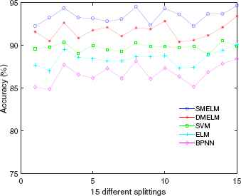
Performance of different algorithms.
4.2. Parameter sensitivity analysis
There are three parameters L, θ and η in the proposed SMELM algorithm. Fig. 6 shows the performance of SMELM with respect to different number of hidden neurons L.

Performance according to the number of neurons.
It can be concluded that in the case of less number of hidden neurons, the accuracy arises quickly when the number of the hidden neurons increases; in the case of large number of hidden neurons, the accuracy is no more sensitive to the increasing of hidden neurons. Therefore, in our experiments, the number of hidden neurons is simply set as 5 times of the feature dimension i.e. L = 650.
As for the remaining two parameters: θ and η, we vary their values from the following exponential sequence {10−10,…,1010}. Fig. 6 shows performance with regard to different combinations of θ and η. It can be found that the optimal values of the parameters are near η = 1 and θ = 10−4, and there is a large flat area near the optimal values. This means SMELM is not very sensitive to the combination of parameters θ and η. A relatively large η can emphasize the samples’ inherent structure information to achieve better performance.
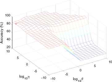
Performance with regard to different combinations of θ and η.
In this paper, we fixed L = 650, η = 1 and θ = 10−4 in the previous experiments.
5. Conclusion
In this paper, a novel approach is proposed for faults diagnosis in sucker rod pumping systems. First, FDCV is employed to extract features of dynamometer cards. Then, a novel model named sparse multi-graph regularized extreme learning machine is proposed and applied as a classifier. In SMELM, two graphs are constructed to explore the inherent structure of data more exactly. The inter-class graph shows the similarity among data from the same class, and the inter-class graph shows the relationship among data from different classes. With the help of these two graphs, the discriminative ability of the ordinary ELM is enhanced. Each graph is obtained through the sparse representation algorithm to avoid the difficulty of choosing the appropriate parameter. The experimental results demonstrate the effectiveness of our method for fault diagnosis in sucker rod pumping systems.
Acknowledgements
This work is partially supported by the National Natural Science Foundation of China (No. 61573088, No. 61573087 and No. 61433004).
References
Cite this article
TY  - JOUR
AU  - Ao Zhang
AU  - Xianwen Gao
PY  - 2018
DA  - 2018/01/01
TI  - Fault diagnosis of sucker rod pumping systems based on Curvelet Transform and sparse multi-graph regularized extreme learning machine
JO  - International Journal of Computational Intelligence Systems
SP  - 428
EP  - 437
VL  - 11
IS  - 1
SN  - 1875-6883
UR  - https://doi.org/10.2991/ijcis.11.1.32
DO  - 10.2991/ijcis.11.1.32
ID  - Zhang2018
ER  -